HAL Id: hal-02485825
https://hal.archives-ouvertes.fr/hal-02485825v2
Submitted on 25 Jan 2021
HAL is a multi-disciplinary open access
archive for the deposit and dissemination of
sci-entific research documents, whether they are
pub-lished or not. The documents may come from
teaching and research institutions in France or
abroad, or from public or private research centers.
L’archive ouverte pluridisciplinaire HAL, est
destinée au dépôt et à la diffusion de documents
scientifiques de niveau recherche, publiés ou non,
émanant des établissements d’enseignement et de
recherche français ou étrangers, des laboratoires
publics ou privés.
Sensitivity equation method for the Navier-Stokes
equations applied to uncertainty propagation
Camilla Fiorini, Bruno Després, Maria Puscas
To cite this version:
Camilla Fiorini, Bruno Després, Maria Puscas. Sensitivity equation method for the Navier-Stokes
equations applied to uncertainty propagation. International Journal for Numerical Methods in Fluids,
Wiley, 2021, �10.1002/fld.4875�. �hal-02485825v2�
Sensitivity equation method for the Navier–Stokes
equations applied to uncertainty propagation
Camilla Fiorini
1, Bruno Després
1, and Maria Adela Puscas
2 1LJLL, Sorbonne Université, Paris, France.
2
CEA, Centre de Saclay, DEN/SAC/DANS/DM2S/STMF/LMSF, Saclay,
France.
Abstract
This works deals with sensitivity analysis for the Navier–Stokes equations. The aim is to provide an estimate of the variance of the velocity field when some of the parameters are uncertain and then to use the variance to compute confidence intervals for the output of the model. First, we introduce the physical model and analyse its stability. The sensitivity equations are derived, and their stability analysed as well. We propose a finite element-volume numerical scheme for the state and the sensitivity, which is integrated into the open-source industrial code TrioCFD. Finally, we present some numerical results: a steady and an unsteady test case for the channel flow problem are investigated. For the steady case, we compare the results to the Monte Carlo method and show how the sensitivity analysis technique succeeds in providing very accurate estimates of the variance. For the unsteady case, a new filtering procedure is proposed to deal with a sensitivity that grows in time. The filtered sensitivity is then used to compute the variance of the output and to provide confidence intervals.
1
Introduction
Sensitivity analysis (SA) studies how changes in the input of a model affect the output, and it is essential for many engineering applications, such as uncertainty quantification, optimal design, and to answer what if questions, i.e. what happens to the solution of the model if the input parameters change. These tasks can be performed in many different ways, depending on the nature of the model considered. In this work, we consider systems that can be modelled with partial differential equations (PDEs). The sensitivity variable itself is defined as the derivative of the state (i.e., the output of the model) with respect to the parameters of interest.
In the framework of PDEs, one can distinguish two main classes of methods: the differentiate-then-discretise methods and the discretise-then-differentiate methods. As the names say, in the first case the state model is formally differentiated with respect to the pa-rameter of interest, providing an analytical sensitivity system which can then be discretised with the most appropriate numerical scheme. The second class of methods swaps the two steps which, in the general case, are not commutative. A detailed comparison between the two classes of methods can be found in [Gun03] for optimisation problems. In this work, we focus on the first class, and, in particular, on the continuous sensitivity equation method [BB97,DPB06,DP06,CDF18,FCD19].
The main aim of this work is to give an estimate of the variance of the solution of the Navier–Stokes equations when there are uncertain parameters and then to use the es-timated variance to compute confidence intervals. This goes under the name of forward uncertainty propagation, which is part of the broader field of uncertainty quantification (UQ). Many strategies and techniques have been proposed in the literature to tackle UQ
problems, particularly in the case of PDEs models: Monte Carlo method [RC13], polynomial chaos [Wal03,XK03,KM06, DPL13], random space partition [AC13], to name but a few. A review of these methods applied to fluid dynamics problems can be found in [WH02].
Methods of uncertainty propagation based on SA are particularly efficient in terms of computational time if compared, for instance, to methods like Monte Carlo. However, since SA is based on Taylor expansions of the state variable with respect to the parameter of interest, these methods are intrinsically local [Del14] : they can be used only for random variables with a small variance. The Monte Carlo approach does not require this assumption; however, it is not applicable for realistic unsteady test cases in 2D and 3D, due to its high computational cost. In this work we propose an approach based on the sensitivity equation method: under the hypothesis of small variance of the input parameters, we can provide a first-order estimate of the variance of the solution at a reasonable computational cost.
Two declinations of the channel flow test case (i.e. study of the flow past an obstacle) are investigated: a steady (Re “ 25) and an unsteady (Re “ 100) test case. For the steady test case, a detailed comparison with the Monte Carlo method is performed: the variance of the output is first estimated using a classical Monte Carlo technique and then with the sensitivity analysis method. The results are extremely accurate. The unsteady test case presents a sensitivity which grows in time: this is caused by the fact that the parameter considered has an infuence on the frequency of vortex shedding. This problem is also described in [HEPB04] for a similar test case to the one considered here: to deal with it, they chose a pulsating inflow velocity, which imposes the frequency of vortex shedding. However, this choice is not suitable for all applications. Therefore we propose a new filtering technique, which allows us to recover the periodic physical part of the sensitivity.
The main original contributions of this work are: (a), to establish the stability in the norm L8p0, T ; L2
pΩqq X L2p0, T ; H1pΩqq for the state and for the sensitivity, we provide an explicit function adapted to the specific geometry to homogenise the Dirichlet boundary conditions (b), we detail the discretisation of the method within a finite element-volume (FEV) framework, well adapted to the open-source industrial code TrioCFD; (c), to be able to remove the phase dependency in the sensitivity signals in the case of pulsating flows, typically in the Von Karman vortex street, we propose and justify a new filtering technique. These results are also validated with a detailed comparison with Monte Carlo simulations. The paper is organised as follows: in section 2 we present the physical model for the state and derive the sensitivity equations. Stability estimates are provided for both the state and the sensitivity for the prescribed boundary conditions. To do that, we introduce a function to homogenise the Dirichlet boundary conditions: the computation of such a function is explicit and detailed in appendix A. In section 3, we design a FEV method for the sensitivity, which is adapted to the open-source industrial code TrioCFD [DC]. In section4, the code implemented for the sensitivity is rigorously validated. In section5, we show how the sensitivity can be used to give a first order estimate of the variance of the model output; then the estimated variance is used to compute confidence intervals for the output of the model. In section6, the numerical results are presented and discussed.
2
The physical model
In this section, we present the physical model as well as some stability estimates for it and its sensitivity.
2.1
The state equations
Let us consider the domain Ω in Figure1: it is a channel with walls on the top and the bottom and an obstacle of square section at distance xD from the inflow boundary. The
Γin Γout Γtop Γbottom Γobst 0 ` y 0 xD L x d `´d 2 `´d 2 0 ` y 0 xD L x d `´d 2 `´d 2 0 ` y 0 xD L x d `´d 2 `´d 2 0 ` y 0 xD L x d `´d 2 `´d 2 0 ` y 0 xD L x d `´d 2 `´d 2 0 ` y 0 xD L x d `´d 2 `´d 2 0 ` y 0 xD L x d `´d 2 `´d 2 0 ` y 0 xD L x d `´d 2 `´d 2 0 ` y 0 xD L x d `´d 2 `´d 2
Figure 1: Domain for the first test case.
$ ’ ’ ’ ’ ’ ’ ’ ’ & ’ ’ ’ ’ ’ ’ ’ ’ % Btu ´ ν∆u ` pu ¨ ∇qu ` ∇p “ f Ω, t ą 0, ∇ ¨ u “ 0 Ω, t ą 0, upx, 0q “ 0 Ω, t “ 0, u “ ´gpyqn on Γin,
u “ 0 on Γw“ ΓobstY ΓtopY Γbottom,
pν∇u ´ pIqn “ 0 on Γout,
(1)
where u “ pux, uy
qt is the velocity, p is the pressure, f the external force and gpyq the prescribed inflow condition. The first equation models the conservation of the momentum and the second one the conservation of the mass. In the following, they will be referred to as, respectively, the momentum equation and the mass equation. We impose no slip boundary condition of the walls of the domain, a prescribed velocity at the inflow and a homogeneous Neumann boundary condition at the outflow.
Remark: the outflow of the domain is not a physical boundary: the physical domain considered is, in some sense, infinite. The outflow boundary is imposed only for numerical computations: this means that we can always choose it far enough from the obstacle in order to have no recirculation at the outflow and therefore u ¨ n|Γoutě 0. In [BZD00] one can find a detailed study on the dependence of the recirculation length on Reynolds number for a confined flow past a square obstacle. We use this condition as hypothesis to prove the stability of the state system.
In the following proposition, we provide a stability estimate for the solution u. To do that, we introduce a function Rg, which we use to homogenise the inflow boundary
conditions. This is also known as a lifting procedure in the mathematical literature. Proposition 1. Let Rg be a sufficiently smooth1 stationary2 function such that ∇ ¨ Rg“
0 in Ω, Rg “ u on ΓinY Γw, and ∇Rgn|Γout “ 0. Then, if u ¨ n| ě 0 on Γout and ˜f is stationary the following stability estimate holds:
~u~2ď }Rg}2` }˜f ptq}2t ` KpRg, ˜f qe2t}∇Rg}L8, (2)
where ˜f “ f ` ν∆Rg´ pRg¨ ∇qRg, and the norm ~ ¨ ~ is defined as follows:
~u~2:“ }upT q}2` 2ν żT
0
}∇uptq}2dt.
Proof. In order to deal with the boundary terms, we start by homogenising the boundary conditions ˜u “ u ´ Rg. We have: ~u~ ď ~˜u~ ` ~Rg~, therefore, since Rg is regular,
controlling ˜u is equivalent to controlling u.
1See sectionAfor how to compute such a function. 2If the boundary conditions depend on time, R
The equations for ˜u are: $ ’ ’ ’ ’ ’ ’ & ’ ’ ’ ’ ’ ’ % Btu ´ ν∆˜˜ u ` pp˜u ` Rgq ¨ ∇q˜u ` p˜u ¨ ∇qRg` ∇p “ ˜f Ω, t ą 0, ∇ ¨ ˜u “ 0 Ω, t ą 0, ˜ upx, 0q “ ´Rg Ω, t “ 0, ˜ u “ 0 on ΓinY Γw, pν∇˜u ´ pIqn “ ´ν∇Rgn “ 0 on Γout.
To obtain the stability estimate, we multiply by ˜u and integrate by parts: ż Ω Btu ¨ ˜˜ u ` ν ż Ω ∇˜u : ∇˜u ` ż Ω rpp˜u ` Rgq ¨ ∇q˜us ¨ ˜u ` ż Ω rp˜u ¨ ∇qRgs ¨ ˜u ´ ż Γin pν∇˜u ´ pIqn ¨ ˜u “ ż Ω ˜f ¨ ˜u. The nonlinear term can be rewritten and integrated by parts as follows:
ż Ω rpp˜u ` Rgq ¨ ∇q˜us ¨ ˜u “ ż Ω p˜u ` Rgq ¨ ∇ ˆ |˜u|2 2 ˙ “ ż BΩ p˜u ` Rgq ¨ n |˜u|2 2 ,
where we used the second equation ∇ ¨ p˜u ` Rgq “ ∇ ¨ u “ 0. Therefore, using the boundary
conditions, one has: 1 2 d dt}˜uptq} 2 ` ν}∇˜u}2` ż Γout p˜u ` Rgq ¨ n ˜ u2 2 ` ż Ω rp˜u ¨ ∇qRgs ¨ ˜u “ ż Ω ˜f ¨ ˜u,
where } ¨ } is the L2-norm in space.
We use the hypothesis p˜u ` Rgq ¨ n|Γout“ u ¨ n|Γoutě 0 to remove the integral on Γout. Then, since Rg is regular, we have:
´ ż Ω rp˜u ¨ ∇qRgs ¨ ˜u ď }∇Rg}L8}˜u}2. Therefore, we obtain: 1 2 d dt}˜u} 2 ` ν}∇˜u}2ď }∇Rg}L8}˜u}2` }˜f }}˜u}. (3) The rest of the proof consists of two steps: first, we prove an estimate for }˜u}; then we substitute this results into (3) to obtain the estimate (2). To obtain an estimate for }˜u}, we start from (3), we remove the positive term ν}∇˜u}2, develop the time derivative, and
simplify }˜u}, which is positive, obtaining: d
dt}˜u} ď }∇Rg}L8}˜u} ` }˜f }, which can be rewritten as:
e´t}∇Rg}L8ˆ d
dt}˜u} ´ }∇Rg}L8}˜u} ˙
ď e´t}∇Rg}L8}˜f }.
We remark that the left-hand side is the time derivative of e´}∇Rg}L8t}˜u}. We can integrate and, if f is constant in time, we obtain:
}˜u} ď ˆ }˜upx, 0q} ` }˜f } }∇Rg}L8 ˙ et}∇Rg}L8 “ ˆ }Rg} ` }˜f } }∇Rg}L8 ˙ et}∇Rg}L8 , (4)
which concludes the first step. For the second step, we start from (3) and use Young’s inequality, obtaining: 1 2 d dt}˜u} 2 ` ν}∇˜u}2ďˆ 1 2` }∇Rg}L8 ˙ }˜u}2`1 2}˜f } 2 .
We multiply by 2 and use the estimate (4), obtaining: d dt}˜u} 2 ` 2ν}∇˜u}2ď }˜f }2` p1 ` 2}∇Rg}L8q ˆ }Rg} ` }˜f } }∇Rg}L8 ˙2 e2t}∇Rg}L8 . Finally, we can integrate in time, obtaining:
}˜u}2` 2ν żt 0 }∇˜upsq}2ds ď }Rg}2` }˜f }2t ` p1 ` 2}∇Rg}L8q ˆ }Rg} ` }˜f } }∇Rg}L8 ˙2 1 2}∇Rg}L8 e2t}∇Rg}L8 .
2.2
The sensitivity equations
We now consider u as a function of space, time and a scalar uncertain parameter a, u “ upx, t; aq and we write a formal Taylor expansion with respect to a:
upx, t; a ` δaq “
8
ÿ
k“0
ukpx, t; aqδak, (5)
where u0“ u and the coefficient ukis the k´th derivative of u with respect to a:
ukpx, t; aq :“
dk
dakupx, t; aq,
and it is called the k´th order sensitivity. To consider more than one parameter of interest, the sensitivity should be defined as the gradient of the state with respect to the vector of parameters and a multi-dimensional Taylor expansion would be necessary, but this is not treated in this work. A similar expansion can be done for the pressure p, and the data f , d, and g. In order to write the equations for the sensitivities, one can replace (5) into (1) and then factorise according to the powers of δa. For k “ 0 we obtain the state system (1). For k “ 1, we obtain the first order sensitivity equations. In this work, we consider only first-order sensitivity and the notation u1 “ ua will be employed. This choice is common
[BB97,DPB06,DP06,CDF18,FCD19] because in most cases first order sensitivities provide enough information. It is possible to consider higher order sensitivities if necessary, but this is not investigated in this work. The first order sensitivity equations, referred to as the sensitivity equations in short, are:
$ ’ ’ ’ ’ ’ ’ ’ ’ & ’ ’ ’ ’ ’ ’ ’ ’ %
Btua´ ν∆ua` pua¨ ∇qu ` pu ¨ ∇qua` ∇pa“ fa Ω, t ą 0,
∇ ¨ ua“ 0 Ω, t ą 0,
uapx, 0q “ 0 Ω, t “ 0,
ua“ ´gapyqn on Γin,
ua“ 0 on Γw,
pν∇ua´ paIqn “ 0 on Γout,
(6)
where Γw:“ ΓobstYΓtopYΓbottom. These are known as the Oseen equations: an introduction
on the subject can be found in [Vol14], both for the theoretical and the numerical aspects. A similar problem is investigated, although only from a numerical point of view, in [DP05,
DPB06], where they use the sensitivity for shape optimization problems: in their case an expansion of the normal n “ř nkpx; aqδak is necessary, which leads to more complicated
boundary conditions. Remark: if ν is considered as the parameter of interest, the second member of the first equation should be fa :“ fa` νa∆u and the Neumann boundary
condition should have the additional term νa∇u n, but this case is not considered in this
We want to obtain a stability estimate for the sensitivity, similar to the one for the state (2). To do this, we need the following hypothesis:
Dκ “ κpu, Ωq ą 0 : ˇ ˇ ˇ ˇ ż Ω rpua¨ ∇qus ¨ ua ˇ ˇ ˇ ˇď κ}ua} 2 . (7)
We remark that hypothesis (7) is trivial if the L8-norm of the gradient ∇u is controlled
(we would have κ “ }∇u}L8). However, in the time dependent case we have a control only on şt0}∇upsq}2ds, which is not sufficient. A similar hypothesis (although less restrictive than ours) can be found in [Ray07]: in the section about linearised Navier–Stokes equations around an instationary state, they suppose
u P L2p0, T ; H1pΩqq X L8p0, T ; L4pΩqq. From the estimate (2) and the triangular inequality we only have
u P L2p0, T ; H1pΩqq X L8p0, T ; L2pΩqq.
Asking for u P L4pΩq @t, would imply having a control on }∇u} @t, because H1pΩq Ă L4pΩq in 2 dimensions (cf. Corollary 9.11 from [Bre10]).
In the following proposition, we provide a stability estimate for the sensitivity.
Proposition 2. Let Rga be a sufficiently smooth stationary function such that ∇ ¨ Rga“ 0 in Ω, Rga“ ua on ΓinY Γw, and ∇Rgan|Γout “ 0 Then, if u ¨ n| ě 0 on Γout and under the hypothesis (7), the following stability estimate holds:
~ua~2ď }Rga} 2 ` }˜fa}2t ` CpRga, ˜fa, κqe 2κt , , where ˜fa“ fa` ν∆Rga´ pRga¨ ∇qRga.
Proof. In order to deal with the boundary terms on Γin, we start by homogenising the
boundary conditions, as we did earlier for the state equations. We define a new variable ˜
ua“ ua´ Rga. The new variable ˜uaverifies the following equations: $ ’ ’ ’ ’ ’ ’ & ’ ’ ’ ’ ’ ’ % Btu˜a´ ν∆˜ua` p˜ua¨ ∇qu ` pu ¨ ∇q˜ua` ∇pa“ ˜fa Ω, t ą 0, ∇ ¨ ˜ua“ 0 Ω, t ą 0, ˜ uapx, 0q “ ´Rga Ω, t “ 0, ˜ ua“ 0 on ΓinY Γw pν∇˜ua´ paIqn “ ´ν∇Rgan “ 0 on Γout.
We can multiply by ua and integrate by parts as done for the state, and we obtain:
1 2 d dt} ˜ua} 2 ` ν}∇ ˜ua}2` ż Ω rp ˜ua¨ ∇qus ¨ ˜ua` ż Ω rpu ¨ ∇q ˜uas ¨ ˜ua“ ż Ω faua. (8)
All the integrals on the boundary are zero thanks to the boundary conditions. For the first integral, we use hypothesis (7) and obtain
ż
Ω
rpua¨ ∇qus ¨ uaě ´κ}ua}2. (9)
The second integral can be treated as we did for the nonlinear term of the state, obtaining: ż Ω rpu ¨ ∇q ˜uas ¨ ˜ua“ ż Ω u ¨ ∇ ˆ | ˜ua|2 2 ˙ “ ż Γout u ¨ n|ua| 2 2 ě 0. (10)
By plugging (9) and (10) into (8), we have: 1 2 d dt} ˜ua} 2 ` ν}∇ ˜ua}2ď κ} ˜ua}2` }˜fa}} ˜ua},
which has exactly the same structure of (3). Therefore, using the same technique, we obtain: } ˜ua}2` 2ν żt 0 }∇ ˜uapsq}2ds ď }Rga} 2 ` }˜fa}2t `1 ` 2κ 2κ ˆ }Rga} ` }˜fa} κ ˙2 e2κt.
3
Numerical schemes
In order to discretise the systems (1) and (6), we use a finite element-volume (FEV) method in space and forward Euler in time. For more details about FEV, cf. [Emo92, Hei03,
APFC17,ABF15]. The numerical schemes described below are implemented in the industrial open source code TRUST TrioCFD [DC].
3.1
Spatial discretisation
Here, we recall the main ideas of the FEV method for the state and we adapt it to the sensitivity equations. For this purpose, in this subsection we only consider the spatial part of the systems (1) and (6) (i.e. Btu “ Btua “ 0). Let ΓD “ ΓinY Γw be the Dirichlet
boundary and ΓN“ Γoutthe Neumann boundary. Let Thbe a triangulation of the domain
Ω compatible with the boundary conditions, and Kj P Th a triangle (j “ 1, . . . , NT): a
triangulation is said to be compatible with the boundary conditions when, if a triangle Kj
has a side on the boundary, than that side belongs entirely to ΓD or entirely to ΓN. We
denote with xi the nodes (i “ 1, . . . , NN), which are the middle points of the edges of the
triangles. A control volume ωiis associated with each node (cf. Figure2for the definition
of ωi).
We introduce the following spaces:
Qh“ tqh: @K P Th, qh|K P P0pKqu,
Vh“ twhcontinuous at xi: @K P Th, wh|KP P1pKqu,
Vh“ twh“ pwx, wyqt: wx, wyP Vhu “ Vh2.
The space Qhis spanned by the indicator functions of the triangles, χK, and Vhis spanned
by ϕipxq, with ϕi P Vh and ϕipxjq “ δij. We look for an approximate solution for the
systems (1) and (6), respectively puh, phq P Vhˆ Qhand pua,h, pa,hq P Vhˆ Qh. The two
components of the discrete velocity field and its sensitivity will be denoted uh“ puxh, u y hq
t
and ua,h“ puxa,h, u y a,hq
t.
In order to have a discrete formulation, we integrate the mass equation and its sensitiv-ity over the triangles Kj and the momentum equation and its sensitivity over the control
volumes ωi: ż BKjzΓD uh¨ n “ ż BKjXΓin g @KjP Th, ´ ż BωizΓN pν∇uh´ phIqn ` ż BωizΓD puhb uhqn “ “ ż ωi f ´ ż BωiXΓin pgn b gnqn @ωi, ż BKjzΓD ua,h¨ n “ ż BKjXΓin ga @KjP Th, ´ ż BωizΓN
pν∇ua,h´ pa,hIqn `
ż BωizΓD pua,hb uh` uhb ua,hqn “ “ ż ωi fa´ ż BωiXΓin pgan b gn ` gn b ganqn @ωi. (11)
Then, one can expand puh, phq and pua,h, pa,hq in the bases of the correspondent spaces as
follows: uhpxq “ NN ÿ i“1 uhpxiqϕipxq, phpxq “ NT ÿ j“1 phpKjqχKj, ua,hpxq “ NN ÿ i“1 ua,hpxiqϕipxq, pa,hpxq “ NT ÿ j“1 pa,hpKjqχKj. (12)
We divide the nodes into two sets: the Dirichlet nodes D :“ ti : xiP ΓDu and all the other
into (11) for the linear terms and using the identity pa b bqc “ apb ¨ cq for the nonlinear terms, we have: $ ’ ’ ’ ’ ’ ’ ’ ’ ’ ’ ’ ’ ’ ’ ’ ’ ’ ’ ’ ’ ’ ’ ’ ’ ’ ’ & ’ ’ ’ ’ ’ ’ ’ ’ ’ ’ ’ ’ ’ ’ ’ ’ ’ ’ ’ ’ ’ ’ ’ ’ ’ ’ % ÿ iPI uhpxiq ¨ ż BKjzΓD ϕin “ ż BKjXΓin g @KjP Th, ´ÿ jPI ż BωizΓN pνuhpxjq b ∇ϕjq n ` NT ÿ j“1 phpKjq ż Bωi χKjn ` ż BωizΓD uhpuh¨ nq “ ż ωi f ´ ż BωiXΓin g2n @ωi, ÿ iPI ua,hpxiq ¨ ż BKjzΓD ϕin “ ż BKjXΓin ga @KjP Th, ´ÿ jPI ż BωizΓN pνua,hpxjq b ∇ϕjq n ` NT ÿ j“1 pa,hpKjq ż Bωi χKjn ` ż BωizΓD ua,hpuh¨ nq ` uhpua,h¨ nq “ ż ωi fa´ 2 ż BωiXΓin ggan @ωi, (13)
We can define the vectors of unknowns as follows:
Uh“ ruxhpxiqsiPI, Vh“ ruyhpxiqsiPI, Ph“ rphpKjqsj“1,...,NT, Uh“ „Uh
Vh
,
Ua,h“ ruxa,hpxiqsiPI, Va,h“ ruya,hpxiqsiPI Pa,h“ rpa,hpKjqsj“1,...,NT, Ua,h“ „Ua,h
Va,h
. We introduce the following vectors:
Fi`“ ż ωi f`´ ż BωiXΓin g2n` Di“ ż BKiXΓin g, Fa i` “ ż ωi fa`´ 2 ż BωiXΓin ggan` Da i“ ż BKiXΓin ga,
and the following matrices: ˜ Ai,j:“ ´ ż BωizΓN ν∇ϕj¨ n Bi,j` :“ ż BKjzΓD ϕin` Ci,j` :“ ż BωizΓN χKjn `
where the superscript ` “ x, y indicates the x´ and y´ components of the normal vector n “ pnx, nyq, of the state source term f “ pfx, fyq, and of the sensitivity source term fa“ pfax, fayq.
For the convection terms, an upwind-type approach is applied: for each edge of Bωi, uh¨n
is computed and, according to its sign, it is multiplied by either uhpxiq or uhpxkq, where ωk
is the control volume adjacent to the considered edge. We remark that using an upwind-type scheme leads to a CFL condition [CFL67] on the time step ∆t when considering the time discretisation: this CFL condition is the same for the state and the sensitivity equations because the transport speed in both equations is u.
For the sake of having a more compact and readable notation, we define x˚as follows:
x˚“
#
xi if uh¨ nią 0 on BωiX Bωk,
xk otherwise,
which truly depends on xi, xk and uh, but we use a simplified notation. The context will
make it non ambiguous. In the same way, we can define xa˚according to the sign of ua,h¨ n.
Therefore, for the convection term in the state equation, we can write: ż Bωi uhpuh¨ nq « ż Bωi uhpx˚qpuh¨ nq “ ż Bωi uhpx˚q ˜ ÿ jPI uhpxjqϕj¨ n ¸ .
We consider the first component of the vector here above: ż Bωi uxhpx˚q ˜ ÿ jPI uhpxjqϕj¨ n ¸ “ “ÿ jPI uxhpxjq ż Bωi uxhpx˚qϕjnx` ÿ jPI uyhpxjq ż Bωi uxhpx˚qϕjny.
We can define the following matrices: Lxi,jpUhq “ ż Bωi uxhpx˚qϕjnx, Lyi,jpUhq “ ż Bωi uxhpx˚qϕjny.
The second component would give as a result Lxi,jpVhq and Lyi,jpVhq. Concerning the
sensi-tivity, doing the same computations would lead to eight matrices, four of them identical to the ones introduced for the state, and four others as follows:
Lxa i,jpUa,hq “
ż
Bωi
uxa,hpxa˚qϕjnx, Lya i,jpUa,hq “
ż Bωi uxa,hpxa˚qϕjny Lxa i,jpVa,hq “ ż Bωi
uya,hpxa˚qϕjnx, Lya i,jpVa,hq “
ż
Bωi
uya,hpxa˚qϕjny
Finally, by introducing the following notation: A “ ˆ˜ A 0 0 A˜ ˙ , B “`Bx By˘ , C “ˆC x Cy ˙ , F “ˆF x Fy ˙ , Fa“ˆF x a Fay ˙ , LpUhq “ˆL x pUhq LypUhq LxpVhq LypVhq ˙ , LapUa,hq “ˆL x apUa,hq LyapUa,hq LxapVa,hq LyapVa,hq ˙ , and observing that C “ Bt, the discrete system can be written in the compact form:
$ ’ ’ ’ & ’ ’ ’ % AUh` BtPh` LpUhqUh“ F, BUh“ D,
AUa,h` BtPa,h` LapUa,hqUh` LpUhqUa,h“ Fa,
BUa,h“ Da.
The first two equations correspond to the state system, and are independent of the last two: the first one is the discretisation of the momentum equation and the second one is the discretisation of the mass equation ∇ ¨ u “ 0, where the vector D accounts for the Dirichlet boundary conditions. The last two equations correspond to the sensitivity and, in particular, the first of these depends on the solution of the state through the convective matrix LpUhq.
3.2
Time discretisation
For the time scheme, we use a forward Euler discretisation [QSS10] with an implicit treat-ment of the diffusion operator: an explicit treattreat-ment would require a very restrictive time step for stability. Let tn be the n´th time step, which is computed according to the CFL condition [CFL67], and let Unh (respectively U
n
a,h) be an approximation of upx, t n
q (re-spectively, uapx, tnq). By coupling this with the spatial scheme described in the previous
subsection, we obtain the following system: $ ’ ’ ’ ’ ’ ’ & ’ ’ ’ ’ ’ ’ % MU n`1 h ´ U n h ∆t ` AU n`1 h ` B t Pn`1h ` LpUnhqU n h“ F n , BUn`1h “ Dn, MU n`1 a,h ´ U n a,h ∆t ` AU n`1 a,h ` B tPn`1
a,h ` LapUna,hqUnh` LpUnhqUna,h“ Fan,
BUn`1a,h “ Dan,
C` Cj ‚ ‚ xi ‚ ‚ ‚ K` Kj ωi
Figure 2: The control volume ωi associated with the node xi is shaded in blue. Cj and C` are
the centres of gravity of the two triangles Kj andK`adjacent to the edge on which xi lies.
where M is the mass matrix with coefficients Mi,j “
ş
ωiϕj. To improve the efficiency in the computations, M is lumped, i.e. it is approximated with a diagonal matrix whose coefficients are |ωi|δi,j. The system (14) is solved with a prediction correction procedure
[Cho68,Tem68,APFC17]. First, an intermediate speed U˚hand its sensitivity U ˚
a,h(which
are not solenoidal) are computed by solving the following systems: pI ` ∆tM´1AqU˚h“ U n h´ ∆tM´1pLpU n hqU n h` B t Pnh´ F n q, pI ` ∆tM´1AqU˚a,h“ U n
a,h´ ∆tM´1pLapUna,hqUnh` LpUhnqUna,h` BtPna,h´ Fanq.
Then, we perform the correction step: Un`1h “ U˚h` ∆tM ´1 BtpPn`1h ´ P n hq, Un`1a,h “ U ˚ a,h` ∆tM´1B t pPn`1a,h ´ P n a,hq. (15)
Finally, by left multiplying by B and imposing the second and fourth equation of (14), one obtains: BM´1BtPn`1h “ BM ´1 BtPnh` Dn`1´ BU˚h ∆t , BM´1BtPn`1a,h “ BM ´1 BtPna,h` Dn`1 a ´ BU˚a,h ∆t , (16)
and Pn`1h and Pn`1a,h can be used to compute Un`1h and Un`1a,h from (15). We remark that in order to solve the pressure problem (16), some technical discrete boundary conditions for the pressure are needed. To do this, in the code TrioCFD [DC] the Neumann boundary condition is split into two parts: the pressure and the gradient of the velocity are set to zero independently of each other.
4
Validation of the implementation of the sensitivity
equation
In order to validate the sensitivity equation method, we consider the following Taylor ex-pansion:
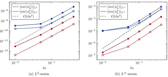
10´2 10´1 10´12 10´11 10´10 10´9 10´8 δa }errpuxhq}L2 }errpuyhq}L2 Opδa2q (a) L2-norm 10´2 10´1 10´7 10´6 10´5 10´4 10´3 δa }errpuxhq}L8 }errpuyhq}L8 Opδa2q (b) L8-norm.
Figure 3: Convergence of the SE method. The symbol ˝ corresponds to the finer mesh (h “ 0.001), the symbol ‚ to the coarser one (h “ 0.002).
and we define the following quantity:
errpuq “ upx, T ; a ` δaq ´ upx, T ; aq ´ δauapx, T ; aq.
If the sensitivity equation are correctly solved, one should have errpuq “ Opδa2q. We considered a straightforward test case: a channel as the one in Figure 1but without the obstacle and with a parabolic velocity profile imposed at the inlet:
gpyq “ 4A `2 yp` ´ yq
The maximal value of the velocity at the inlet is the parameter of interest a (i.e. a “ A). We solved this on two Cartesian grids with h “ 0.001 and h “ 0.002. In Figure 3, we show the L2 and L8 norms for the two components of the velocity on the two different
meshes: for larger δa we observe the expected convergence rate, but starting at δa » 0.05 the curve flattens (especially the ones corresponding to the horizontal component of the velocity). This is due to the fact that the quantity shown is errpuhq and not errpuq: the
spatial discretisation is an additional source of error, and this part of the error is constant for a given mesh, therefore the curve tend to a plateau. The plateau value is smaller for finer meshes, as one can observe in Figure3.
5
Uncertainty propagation
In this section, we want to show how the sensitivity can be used to give a first order estimate of the variance of the model output. In this context, the parameter a is a random variable with a known distribution, expected value µa, and variance σa2. Let Xpx, t; aq be a physical
variable (i.e. the horizontal or vertical velocity, or the pressure), whose expected value µX
and variance σ2
X we want to estimate. To do this, we start from a Taylor expansion of X
with respect to the parameter a centred in the expected value of a, µa:
Xpx, t; aq “ Xpx, t; µaq ` pa ´ µaqXapx, t; aq ` op|a ´ µa|2q, (17)
where Xa“ BaX is the sensitivity of X with respect to the parameter a. Computing the
expected value of the right and left-hand side of (17), one obtains the following first order estimate:
parameter ` L xD d
value 0.7 2 0.4 0.1
Table 1: Values of the domain parameters used in simulations.
Using again the Taylor expansion (17) and the estimate just obtained for the average (18), we obtain an estimate of the variance:
σX2px, tq “ ErpXpx, t; aq ´ µXpx, tqq2s » Erpa ´ µaq2sXa2px, t; aq “ σ 2 aX
2
apx, t; aq. (19)
The estimates (18)-(19) are valid only where the Taylor expansion (17) holds, i.e. for small variances of the random parameter σ2
a. However, one can have an estimate of the variance
with just one simulation of the state and one of the sensitivity, which is a minimal com-putational cost when compared to methods such as Monte Carlo that require thousands of simulations of the state to estimate the variance. In the general case, when more than one parameter is uncertain, to provide an estimate of the variance, one would need one simulation for the state and as many simulations of the sensitivity as the number of uncer-tain parameters [Fio18]. This makes the sensitivity approach really affordable and highly competitive when the number of uncertain parameters is small enough. In the next subsec-tion, we compare the results of the SA approach with the well-known Monte Carlo method [RC13].
The estimated variance can be used for multiple purposes. In this work, we use it to compute some confidence intervals for the physical variables, i.e. find an interval CIX such
that the probability that X falls into CIX is bigger that 1 ´ α. Standard choices for α are
0.05 or 0.01. If the distribution of the random variable X is known, some precise estimates for the extrema of the interval exist. However, SA does not provide any insight of what the distribution of the output is. Therefore we start from Chebyshev inequality [JP12], which states that for any random variable with finite expected value and variance
P p|X ´ µX| ě λq ď
σX2
λ2.
By imposing the desired level for confidence interval, i.e. α “ σX2
λ2, one gets λ “ σX ? α, therefore CIX “ „ µX´ σX ? α, µX` σX ? α . (20)
6
Numerical results
The domain used for the numerical simulations is the one in Figure1, and the values of the parameters are the ones in Table1. The equations are solved on the mesh with a spatial step varying from 0.005 to 0.01. Finally, we consider the following parabolic inflow condition:
gpyq “ 4A
`2 ypy ´ `q, (21)
where A is the maximal value of the inflow velocity, and it is the uncertain parameter (i.e. a “ A). A is a Gaussian random variable of average µA and variance σ2A.
6.1
Steady test case
For this first test case, we consider a small inflow velocity, µA“ 0.25, which corresponds to
Re “ 25 and leads to a stationary solution. The probability density function of A is shown in Figure4: the standard deviation σA“ 7.5 ˆ 10´3is small enough to apply the sensitivity
method described above to compute the variance of the output.
In Figure5, we show the numerical results for the horizontal velocity and its sensitivity. For this test case, we were able to make a Monte Carlo approach as well: 1300 simulations
0.21 0.23 0.25 0.27 0.29 0 1 2 3 4 ·104 95% Pdf of random variable A
Figure 4: Probability density function of the uncertain parameterA.
0 0.075 0.15 0.225 0.3 x axis 1.5 1 0.5 y axis 0.1 0.2 0.3 0.4 0.5 0.6
(a) Horizontal velocity
-0.1629 0.191 0.5448 0.8986 1.252 y axis 0.1 0.2 0.3 0.4 0.5 0.6 x axis 1.5 1 0.5
(b) Sensitivity of the horizontal velocity
0 0.5 1 1.5 2 6 7 8 9 ¨10´3 x
(a) Standard deviation of ux
0 0.5 1 1.5 2 0 0.5 1 1.5 ¨10´3 x SA MC (b) Standard deviation of uy
Figure 6: Standard deviation on the horizontal cross section y “ 0.2. Comparison between
Monte Carlo (MC) and the SA estimate.
0 0.2 0.4 0.6 0 2 4 6 8 ¨10´3 y
(a) Standard deviation of ux
0 0.2 0.4 0.6 0 1 2 3 4 ¨10´4 y SA MC (b) Standard deviation of uy
Figure 7: Standard deviation on the vertical cross section x “ 1. Comparison between Monte
Carlo and the SA estimate.
of the state were necessary. In Figures6-7, we compare the variance estimated using the sensitivities and the one computed with Monte Carlo on two cross sections of the domain. As one can see, the two strategies give very similar results. In Figures8-9, we show the confidence intervals computed according to (20) for α “ 0.05: in blue the confidence intervals are obtained with the average and variance estimated with SA, in red with Monte Carlo.
For this test case, the first order approximations provided by the SA are more than satisfactory: with only two simulations, we obtain results comparable to the ones obtained with the Monte Carlo approach, which requires 1300 simulations.
6.2
Unsteady test case
We now consider a case with a higher Reynolds number (Re “ 100, which corresponds to µA “ 1); thus, we are in the range in which a Von Karman vortex street occurs. In this
situation, it is reasonable to assume that the velocity behaves as follows: upx, t; aq »
N
ÿ
k“0
0 0.5 1 1.5 2 0.2
0.25 0.3
x
(a) Confidence interval for ux
0 0.5 1 1.5 2 8 6 4 2 0 2 ·10 2 x
(b) Confidence interval for uy
Figure 8: Confidence intervals on the horizontal cross sectiony “ 0.2, with α “ 0.05. Comparison
between Monte Carlo and the SA approaches.
0 0.2 0.4 0.6 0
0.1 0.2
y
(a) Confidence interval for ux
0 0.2 0.4 0.6 2 1 0 1 2·10 2 y
(b) Confidence interval for uy
Figure 9: Confidence intervals on the vertical cross section x “ 1, with α “ 0.05. Comparison
0 1 2 3 4 0.4 0.2 0 0.2 0.4 0.6 t State in x = (1, 0.35) 0 1 2 3 4 0.2 0.1 0 0.1 t State in x = (0.6, 0.35) 0 1 2 3 4 0 0.5 1 t State in x = (1, 0.2) ux uy
Figure 10: Velocity field in three different points of the domain with respect to time.
0 1 2 3 4 20 10 0 10 20 t Sensitivity in x = (1, 0.35) 0 1 2 3 4 5 0 5 t Sensitivity in x = (0.6, 0.35) 0 1 2 3 4 5 0 5 t Sensitivity in x = (1, 0.2) ux a uy a
Figure 11: Sensitivity of the velocity field in three different points of the domain with respect to time.
We remark that (22) does not solve (1) exactly: some terms have been neglected. Although, from physical knowledge of the phenomenon and looking at numerical results downstream to the obstacle, we can say that the hypothesis (22) is reasonable and that N can be as small as 2 or 3.
To simulate this test case, we use the following procedure: first, we simulate the state until it reaches a periodic solution of the form (22); then, this state is injected into the sensitivity equations and the sensitivity simulation is run.
We remark that by differentiating (22) with respect to the parameter a, one obtains the following behaviour for the sensitivity:
uapx, t; aq “ N
ÿ
k“0
u0,a,kpx; aq cospωkpaqtq ´ t N
ÿ
k“0
u0,kpx; aqωk1paq sinpωkpaqtq. (23)
We can distinguish two contributions: the first sum corresponds to the influence that the input parameter a has on the amplitude of the oscillations u0,k, the second sum corresponds
to the influence on the the frequency ωpaq. The second effect leads to a sensitivity that grows linearly in time and difficult to work with. This problem is described in [HEPB04] for a similar test case: to deal with it, they chose a pulsating inflow velocity, which imposes the frequency of vortex shedding (i.e. ωk does not depend on a). However, this choice is
not suitable for all applications. This is why, in the next subsection, we propose a filter to recover the first part of the sensitivity (23).
In Figures10-11, we show the state and sensitivity in different points of the domain: as one can see, hypotheses (22) and (23) are verified.
0 5 10 15 0 0.02 0.04 0.06 0.08 0.1 0.12 0.14 0 5 10 15 0 0.002 0.004 0.006 0.008 0.01 0.012 0 5 10 15 0 0.02 0.04 0.06 0.08 0.1 0.12 0.14 0 5 10 15 0 0.02 0.04 0.06 0.08 0.1 0.12 0.14 0 5 10 15 0 0.05 0.1 0.15 0.2 0 5 10 15 0 0.02 0.04 0.06 0.08 0.1 0.12 0.14
Figure 12: Fourier transform of the velocity in three different points. Top row: horizontal
component. Bottom row: vertical component.
6.2.1 Filter
In this subsection, we propose a filter to recover the bounded part of the sensitivity
hpx, t; aq :“
N
ÿ
k“0
u0,a,kpx; aq cospωkpaqtq.
To the best of our knowledge, this is the first work in which a filtering procedure is proposed in this context. We focus on this part of the sensitivity because, for industrial applications, the variance of the amplitude of the oscillations is more interesting than the variance of their phase.
We suppose that the ratio between the ωkis rational, i.e. that the state (22) and h are
periodic in time. By computing the discrete Fourier transform of the state we can see that not only this is true, but also that we have a fundamental frequencyω and then multiples of that, 2ω, 3ω. In Figure12, only the second harmonic 2ω is visible. One can identify the period T of the state using the Fourier transform, and therefore @t the following equality holds: żt t´T uapx, s; aq s ds “ żt t´T hpx, s; aq s ds “: Iptq. (24)
The left-hand side of (24) can be computed numerically. To obtain hpx, t; aq, one can compute the derivative of Iptq and use the fact that h is T -periodic in time:
dI dt “ hpx, t; aq t ´ hpx, t; aq T ´ t , (25)
and finally one has
hpx, t; aq “ tpT ´ tq T
dI dt.
The derivative (25) can be computed numerically by finite differences. In Figure 13, we applied the filter just described to a case where ua and h are known analytically: as one
can see in the left Figure, the filter precision degrades with time. However, since we know that h is periodic, one can consider the first period and repeat it, which is what is shown in the right Figure. Of course, this leads to a small jump where the two periods are glued together.
0 5 10 15 20 25 30 -3 -2 -1 0 1 2 3 0 5 10 15 20 25 30 -2 -1 0 1 2 3
Figure 13: Filter applied to an analytical case.
We remark that this filter could be build on multiple periods as well. However, some considerations on the computational costs are necessary: in order to filter on N periods, one has to run the simulation for at least N ` 1 periods. We tested the filter on multiple periods and the differences observed do not justify the additional computational cost for this test case. The following results are obtained using a one-period filter.
In Figure 14, we show the results of the filter applied to the sensitivities shown previ-ously (Figures10-11). The sensitivities obtained in this way can now be used for different applications such as, for instance, the computation of a confidence interval as done in the previous section (cf. Figure15). However, one must be careful, as the filtered sensitivities take into account only the variance of the amplitude of the oscillations and not the variance of the frequency.
7
Conclusion
In this paper, we propose an efficient computational strategy to deal with problems of uncertainty propagation for the Navier–Stokes equations. First, the state equations are presented, and the sensitivity equations are derived according to the continuous sensitivity equation method. Stability estimates in L8p0, T ; L2pΩqqXL2p0, T ; H1pΩqq for both the state and the sensitivity are rigorously proven. We homogenise the Dirichlet inflow boundary conditions using an auxiliary function which is explicitly computed. A FEV numerical scheme is designed for the sensitivity and implemented in the open-source code TrioCFD. A classical test case of flow past a square-section cylinder is investigated in two different regimes: a steady case (Re “ 25) and a Karman vortex street (Re “ 100). For both cases, the sensitivity is used to estimate the variance of the velocity field, and 95% confidence intervals are computed. In the steady case, a detailed comparison with a Monte Carlo method is performed: the results of the sensitivity based method are extremely accurate, and the computational gain is significant. The unsteady test case raises an issue: due to the periodic nature of the velocity, the sensitivity grows in time and is therefore unusable. We propose a new procedure, which consists in filtering the different contributions to the sensitivity in order to recover its physical parts. The filtered sensitivity is then used to compute the confidence intervals.
Questions such as the investigation of different parameters of interest, 3´dimensional computations, the addition of the energy equation to deal with the temperature and the extension to the unsteady Reynolds-Averaged Navier–Stokes (URANS) equations for the study of turbulent flows will be addressed in future works, to tackle more realistic problems.
0 1 2 3 4 10 5 0 5 10 t ux ain x = (1, 0.35) Unfiltered Filtered 0 1 2 3 4 1 0.5 0 0.5 t ux ain x = (0.6, 0.35) 0 1 2 3 4 6 4 2 0 2 4 6 t ux ain x = (1, 0.2) 0 1 2 3 4 20 10 0 10 20 t uy ain x = (1, 0.35) 0 1 2 3 4 5 0 5 t uy ain x = (0.6, 0.35) 0 1 2 3 4 6 4 2 0 2 4 t uy ain x = (1, 0.2)
Figure 14: Filter applied to the sensitivity of the velocity in three different points of the domain. Top row: horizontal component. Bottom row: vertical component.
0 0.2 0.4 0.6 0.8 1 1.2 1.4 0.4 0.45 0.5 0.55 0.6 0.65 t
Confidence interval for uxin x = (1, 0.35)
0 0.2 0.4 0.6 0.8 1 1.2 1.4 0.19 0.18 0.17 0.16 0.15 0.14 t
Confidence interval for uxin x = (0.6, 0.35)
0 0.2 0.4 0.6 0.8 1 1.2 1.4 0.8 0.9 1 1.1 t
Confidence interval for uxin x = (1, 0.2)
0 0.2 0.4 0.6 0.8 1 1.2 1.4 0.2
0 0.2
t
Confidence interval for uyin x = (1, 0.35)
0 0.2 0.4 0.6 0.8 1 1.2 1.4 0.2 0.1 0 0.1 0.2 t
Confidence interval for uyin x = (0.6, 0.35)
0 0.2 0.4 0.6 0.8 1 1.2 1.4 0.1 0 0.1 0.2 t
Confidence interval for uyin x = (1, 0.2)
Figure 15: Confidence intervals (α “ 0.05) for the velocity in three different points of the domain. Top row: horizontal component. Bottom row: vertical component.
Appendix
A
Computation of the auxiliary function R
gpx, yq
We need a vector field Rgpx, yq “ pRxgpx, yq, Rygpx, yqqt which is solenoidal, smooth enough
(at least continuous with ∇RgP L8pΩq) and equal to u on the Dirichlet boundary, i.e. on
ΓinY Γw. The same can be done for ua, in particular, for the inflow boundary condition
used in this work (21).
First of all, one needs to define a function gFpyq with the following properties:
gFp0q “ gFp`q “ 0, gFpyq “ 0 @y P„ ` ´ d 2 , ` ` d 2 , (26) gF P C0r0, `s, BygF P L8r0, `s ż` 0 gFpyqdy “ ż` 0 gpyqdy. (27)
This is easy and a function with these properties will be specified later. Let Hpxq be a C2 function such that
Hp0q “ 1, Hpxq “ 0 @x P rxD, Ls, H1p0q “ H1pxDq “ 0.
Many different options are possible for Hpxq. Let Gpyq (respectively GFpyq) be a primitive
of gpyq (respectively gFpyq):
Gpyq “ ży 0 gpsqds GFpyq “ ży 0 gFpsqds. (28)
Proposition 3. The following vector field is solenoidal, continuous and equals u at the boundary:
Rxgpx, yq “ gpyqHpxq ` gFpyqp1 ´ Hpxqq Rygpx, yq “ ´H1pxqpGpyq ´ GFpyqq.
Furthermore, ∇Rg P L8pΩq and ∇Rgn|Γout“ 0. Proof. (i) The field is solenoidal:
∇ ¨ Rg“ BxRxg` ByRyg “ gpyqH 1
pxq ´ gFH1pxq ´ H1pxqpgpyq ´ gFpyqq “ 0.
(ii) The field is continuous because each component is a product and sum of continuous functions.
(iii) The field equals u on ΓD.
(a) The x component of u is equal to gpyq on Γin and zero on ΓDzΓin. On Γin, we
have:
Rxgp0, yq “ gpyqHp0q ` gFpyqp1 ´ Hp0qq “ gpyq,
because Hp0q “ 1. On Γtopand Γbottom,
Rgxp`, yq “ R x
gp0, yq “ 0
because gp0q “ gp`q “ 0 and gFp0q “ gFp`q “ 0. Finally, on the obstacle we have
Rxgpx, yq “ gFpyq, which is zero @y P“`´d2 , ``d 2 ‰ thanks to property (26).
(b) The y component of u is zero on ΓD. On Γin we have
Rygp0, yq “ 0,
because H1p0q “ 0. On the bottom wall y “ 0, we have
Rygpx, 0q “ ´H1pxqpGp0q ´ GFp0qq “ 0,
because Gp0q “ GFp0q “ 0, from (28). On the top wall y “ `:
Rygpx, `q “ 0,
because Gp`q “ GFp`q thanks to the property (27). Finally, on the obstacle we
have
Rygpx, yq “ 0,
because H1pxq “ 0@x P rx D, Ls.
(iv) ∇RgP L8pΩq and ∇Rgn|Γout“ 0. The gradient of Rg is the following:
∇Rgpx, yq “
„ H1
pxqpgpyq ´ gFpyqq pg1pyq ´ gF1 pyqqHpxq ` g1Fpyq
´H2pxqpGpyq ´ GFpyqq ´H1pxqpgpyq ´ gFpyqq
(29) which is in L8pΩq thanks to the hypotheses of regularity of H and g
F. Finally, on the
outflow boundary the normal is n “ p1, 0qt. If we evaluate (29) on Γ
out, i.e. x “ L, we have: ∇RgpL, yq “ „0 g1 Fpyq 0 0 , and therefore ∇Rgn|Γout“ 0.
Example of an auxiliary function for the state
Let g and its primitive G be the following functions: gpyq “ yp` ´ yq, Gpyq “ `
2y 2 ´1 3y 3 . Then, we can define the function gF as follows:
gFpyq “ $ ’ & ’ % ky``´d 2 ´ y ˘ y P“0,`´d 2 ˘ , 0 y P“`´d2 , ``d 2 ‰ , kp` ´ yq`y ´ ``d 2 ˘ y P```d 2 , `‰ ,
where k is chosen in order to respect the property (27) and it is k “ 4`
3 p` ´ dq3. The primitive GF is: GFpyq “ $ ’ ’ & ’ ’ % k`´d 4 y 2 ´ ky33 y P“0,`´d 2 ˘ , ` 12 y P “`´d 2 , ``d 2 ‰ , ` 12´ k ´ y3 3 ´ 3``d 4 y 2 ``p``dq2 y ¯ ´ k```d2 ˘2`d´5`12 ˘ y P```d 2 , `‰ .
Finally, we chose the following function for Hpxq:
Hpxq “ $ & % 2 ´ x xD ¯3 ´ 3 ´ x xD ¯2 ` 1 x P r0, xDs, 0 x P pxD, Ls,
which has all the required properties. The auxiliary function just computed is shown in Figure16. Figure17shows the two components of Rg, Rxg and Ryg.
Figure 16: Solenoidal field from the example.
References
[ABF15] P.-E. Angeli, U. Bieder, and G. Fauchet. Overview of the TrioCFD code: main features, V&V procedures and typical applications to nuclear engineering. Nureth. 16. Chicago, USA, page 252, 2015.
[AC13] Remi Abgrall and Pietro Marco Congedo. A semi-intrusive deterministic ap-proach to uncertainty quantification in non-linear fluid flow problems. Journal of Computational Physics, 235:828–845, 2013.
[APFC17] P. E. Angeli, M. A. Puscas, G. Fauchet, and A. Cartalade. FVCA8 Benchmark for the Stokes and Navier–Stokes equations with the TrioCFD code - Benchmark session. In International Conference on Finite Volumes for Complex Applica-tions, pages 181–202. Springer, 2017.
[BB97] J. Borggaard and J. Burns. A PDE sensitivity equation method for optimal aerodynamic design. Journal of Computational Physics, 136(2):366 – 384, 1997. [Bre10] H. Brezis. Functional analysis, Sobolev spaces and partial differential equations.
Springer Science & Business Media, 2010.
[BZD00] J. Breuer, M .and Bernsdorf, T. Zeiser, and F. Durst. Accurate computations of the laminar flow past a square cylinder based on two different methods: lattice-Boltzmann and finite-volume. International journal of heat and fluid flow, 21(2):186–196, 2000.
[CDF18] C. Chalons, R. Duvigneau, and C. Fiorini. Sensitivity analysis and numerical diffusion effects for hyperbolic PDE systems with discontinuous solutions. The case of barotropic Euler equations in Lagrangian coordinates. SIAM Journal on Scientific Computing, 40(6):A3955–A3981, 2018.
[CFL67] R. Courant, K. Friedrichs, and H. Lewy. On the partial difference equations of mathematical physics. IBM journal of Research and Development, 11(2):215– 234, 1967.
[Cho68] A. J. Chorin. Numerical solution of the navier-stokes equations. Mathematics of computation, 22(104):745–762, 1968.
[DC] DEN-CEA. TRUST TrioCFD code.
[Del14] C. Delenne. Propagation de la sensibilité dans les modèles hydrodynamiques., 2014.
[DP05] R. Duvigneau and D. Pelletier. Evaluation of nearby flows by a shape sensitivity equation method. In 43rd AIAA Aerospace Sciences Meeting and Exhibit, page 127, 2005.
[DP06] R. Duvigneau and D. Pelletier. A sensitivity equation method for fast evaluation of nearby flows and uncertainty analysis for shape parameters. International Journal of Computational Fluid Dynamics, 20(7):497–512, 2006.
[DPB06] R. Duvigneau, D. Pelletier, and J. Borggaard. An improved continuous sensitiv-ity equation method for optimal shape design in mixed convection. Numerical Heat Transfer, Part B: Fundamentals, 50(1):1–24, 2006.
[DPL13] Bruno Després, Gaël Poëtte, and Didier Lucor. Robust uncertainty propagation in systems of conservation laws with the entropy closure method. In Uncertainty quantification in computational fluid dynamics, pages 105–149. Springer, 2013. [Emo92] P. Emonot. Méthodes de volumes éléments finis: applications aux équations de
Navier Stokes et résultats de convergence. PhD thesis, Lyon 1, 1992.
[FCD19] C. Fiorini, C. Chalons, and R. Duvigneau. A modified ensitivity equation method for Euler equations in presence of shocks. Numerical methods for partial differ-ential equations, 2019.
[Fio18] C. Fiorini. Sensitivity analysis for nonlinear hyperbolic systems of conservation laws. PhD thesis, Université Paris Saclay, 2018.
[Gun03] M. D. Gunzburger. Perspectives in flow control and optimization, volume 5. Siam, 2003.
[Hei03] S. Heib. Nouvelles discrétisations non structurées pour des écoulements de fluides à incompressibilité renforcée. PhD thesis, Paris 6, 2003.
[HEPB04] H. Hristova, S. Etienne, D. Pelletier, and J. Borggaard. A continuous sensitivity equation method for time-dependent incompressible laminar flows. International Journal for Numerical Methods in Fluids, 50:817–844, 2004.
[JP12] J. Jacod and P. Protter. Probability essentials. Springer Science & Business Media, 2012.
[KM06] O.M. Knio and O.P. Le Maitre. Uncertainty propagation in CFD using polyno-mial chaos decomposition. Fluid Dynamics Research, 38(9):616–640, September 2006.
[QSS10] A. Quarteroni, R. Sacco, and F. Saleri. Numerical mathematics, volume 37. Springer Science & Business Media, 2010.
[Ray07] J-P Raymond. Stokes and Navier–Stokes equations with nonhomogeneous boundary conditions. Annales de l’Institut Henri Poincaré - Analyse Non Linéaire, 24(6):921–951, 2007.
[RC13] C. Robert and G. Casella. Monte Carlo statistical methods. Springer Science & Business Media, 2013.
[Tem68] R. Temam. Une méthode d’approximation de la solution des équations de navier-stokes. Bulletin de la Société Mathématique de France, 96:115–152, 1968. [Vol14] J. Volker. Lecture notes on numerical methods for incompressible flow problems
II,Chapter 4, 2014.
[Wal03] R. Walters. Towards stochastic fluid mechanics via polynomial chaos. In 41st AIAA Aerospace Sciences Meeting and Exhibit, Reno, USA, 2003.
[WH02] R. W. Walters and L. Huyse. Uncertainty analysis for fluid mechanics with applications. Technical report, National aeronautics and space administration, Hampton, VA, Langley research center, 2002.
[XK03] D. Xiu and George E. Karniadakis. Modeling uncertainty in flow simulations via generalized polynomial chaos. Journal of computational physics, 187(1):137–167, 2003.