Modelling glacier-bed overdeepenings and possible future lakes for
the glaciers in the Himalaya–Karakoram region
A. LINSBAUER,
1,2H. FREY,
1W. HAEBERLI,
1H. MACHGUTH,
3M.F. AZAM,
4,5S. ALLEN
1,6 1Department of Geography, University of Zürich, Zürich, Switzerland 2Department of Geosciences, University of Fribourg, Fribourg, Switzerland 3
Centre for Arctic Technology, Danish Technical University, Lyngby, Denmark 4
School of Environmental Sciences, Jawaharlal Nehru University, New Delhi, India 5
IRD/UJF – Grenoble I/CNRS/G-INP, LGGE UMR 5183, LTHE UMR 5564, Grenoble, France 6
Institute of Environmental Sciences, University of Geneva, Switzerland Correspondence: Andreas Linsbauer <[email protected]>
ABSTRACT. Surface digital elevation models (DEMs) and slope-related estimates of glacier thickness enable modelling of glacier-bed topographies over large ice-covered areas. Due to the erosive power of glaciers, such bed topographies can contain numerous overdeepenings, which when exposed following glacier retreat may fill with water and form new lakes. In this study, the bed overdeepenings for
�28 000 glaciers (40 775 km2) of the Himalaya–Karakoram region are modelled using GlabTop2 (Glacier Bed Topography model version 2), in which ice thickness is inferred from surface slope by parameterizing basal shear stress as a function of elevation range for each glacier. The modelled ice thicknesses are uncertain (�30%), but spatial patterns of ice thickness and bed elevation primarily depend on surface slopes as derived from the DEM and, hence, are more robust. About 16 000 overdeepenings larger than 104m2were detected in the modelled glacier beds, covering an area of
�2200 km2and having a volume of �120 km3(3–4% of present-day glacier volume). About 5000 of these overdeepenings (1800 km2) have a volume larger than 106m3. The results presented here are useful for anticipating landscape evolution and potential future lake formation with associated opportunities (tourism, hydropower) and risks (lake outbursts).
KEYWORDS: glacial geomorphology, glaciological model experiments, processes and landforms of
glacial erosion
1. INTRODUCTION
Modelling detailed glacier-bed topographies and producing digital elevation models (DEMs) ‘without glaciers’ (Linsbauer and others, 2009) have become possible with the combined use of digital terrain information and slope-related estimates of glacier thickness. Distributed ice thickness estimates are now available at both regional (Farinotti and others, 2009; Linsbauer and others, 2012; Clarke and others, 2013) and global scales (Huss and Farinotti, 2012). These approaches mainly relate local glacier thickness to surface slope via the basal shear stress satisfying the inverse flow law for ice, but use parameterization schemes of variable complexity (cf. the intercomparison by Frey and others 2014).
An important application of such investigations is the prediction of future landscape evolution and lake formation in deglaciating mountain chains (Frey and others, 2010; Linsbauer and others, 2012). As the erosive power of glaciers can form numerous and sometimes large closed topographic depressions, many overdeepenings are com-monly found in formerly glaciated mountain ranges (Hooke, 1991; Cook and Swift, 2012). New lakes develop where such overdeepened areas become exposed and filled with water rather than sediments (Frey and others, 2010). In the Swiss Alps, for instance, 500–600 overdeepenings were modelled in the beds of extant glaciers (Linsbauer and others, 2012). For a single glacier, these overdeepenings were confirmed by independent modelling and measure-ments (Zekollari and others, 2013, 2015).
The present analysis emphasizes modelled overdeepen-ings underneath the present-day glaciers and thus provides information about potential future lakes for �28 000 glaciers in the Himalaya–Karakoram (HK) region. This study builds on the work of Frey and others (2014), who modelled the total volume and thickness distribution of all HK glaciers, by focusing specifically on the location and geometry of bed overdeepenings. Such information forms the basis for assessing possible impacts and opportunities related to the potential future lakes (e.g. hydropower, tourism, outburst hazards; Yamada and Sharma, 1993; Bajracharya and Mool, 2010; Künzler and others, 2010; Terrier and others, 2011; Haeberli and Linsbauer, 2013; Loriaux and Casassa, 2013; Schaub and others, 2013).
2. STUDY REGIONS AND DATA
Following Bolch and others (2012) and Frey and others (2014) the HK region is divided into four sub-regions: the Karakoram, and the western, central and eastern Himalaya (Fig. 1; cf. Gurung, 1999; Shroder, 2011). Glacier bed topographies are calculated for all glaciers in all four sub-regions. For each sub-region, a test area is chosen to visualize and discuss the results:
1. For the Karakoram the test region is located between K2 and the Karakoram Pass in the borderland of India, Pakistan and China. This test region, covering a wide
elevation range (3500–8000 m a.s.l.), is dominated by the largest glaciers in the HK region (e.g. Siachen glacier (�72 km long) and Baltoro glacier (�64 km)). These two compound glaciers comprise a large number of tributary glaciers, and both end in large, very thick and flat (partly) debris-covered glacier tongues, flowing southeast (Sia-chen) and west (Baltoro). The Karakoram is also known for a large number of surge-type glaciers on the northern slope of the main ridge, heading in directions north to west (Barrand and Murray, 2006; Bhambri and others, 2013; Rankl and others, 2014).
2. In the western Himalaya the test region in the Pir Panjal range, Himachal Pradesh, India, is located in the monsoon–arid transition zone (Gardelle and others, 2011), where glaciers are influenced by both the Indian summer monsoon and the westerlies (Bookhagen and Burbank, 2006, 2010). Chhota Shigri and Bara Shigri glaciers belong to the Chandra valley on the northern slopes of the Pir Panjal range in the Lahaul and Spiti District of Himachal Pradesh. Bara Shigri (�28 km) is the largest glacier in Himachal Pradesh, and has a heavily debris-covered tongue (Berthier and others, 2007). Chhota Shigri glacier is part of a long-term monitoring programme (Wagnon and others, 2007; Azam and others, 2014). On the southern slope of the Pir Panjal range, numerous smaller and larger (hanging, mountain and valley) glaciers flow down the steep rocky slopes of the narrow Parbati valley. Some glacier tongues reaching the valley floors at �4000 m a.s.l. are debris-covered. 3. The test area in the central Himalaya is located in the
Khumbu Himal, eastern Nepal, around Mount Everest. The topography here is characterized by huge relief and steep slopes. The valleys are filled by large debris-covered glacier tongues that extend down to 5000 m a.s.l., often with supraglacial ponds, ice cliffs and thermokarst features (Bolch and others, 2008). Development of supra-or proglacial lakes is widespread, an example being Imja lake which has grown rapidly since the 1960s (Chikita and others, 2000; Fujita and others, 2009;
Somos-Valenzuela and others, 2014) and has caused concern regarding outburst flood hazards (Quincey and others, 2007; Bajracharya and Mool, 2010).
4. The test region for the eastern Himalaya comprises the northernmost section of the Bhutan Himalayan main ridge, with the highest peaks at �7300 m a.s.l. The northern glaciers originate from firn/ice plateaus located at �7000 m a.s.l. and flow with gentle slopes and clean ice towards elevations around 5000 m a.s.l. on the Tibetan Plateau, where proglacial lakes can be found (Kääb, 2005). The southern glaciers descend to eleva-tions at �4000 m a.s.l., originating from large and steep headwalls which provide enough debris to produce a thick cover on the more or less stagnant tongues (Bolch and others, 2012).
There are several reasons for choosing these test regions. The Karakoram test region contains the largest glaciers in HK. In the Pir Panjal range, western Himalaya, in situ thickness measurements are available and a range of different glacier sizes are found. There are well-known, studied and documented glaciers and glacial lakes around Mount Everest in the central Himalaya region, and the eastern Himalayan region features large geomorphological variations between clean, gently sloping north-facing gla-ciers and steep, debris-covered south-facing valley glagla-ciers. Here we use the same glacier outlines as in Bolch and others (2012) and Frey and others (2014). The outlines have been compiled from satellite scenes acquired between 2000 and 2010. Data from the following sources are used: the International Centre for Integrated Mountain Development (ICIMOD; Bajracharya and Shrestha, 2011), the GlobGlacier project (Frey and others, 2012), the first Chinese Glacier Inventory (Shi and others, 2010) and Bhambri and others (2013) (Fig. 1). Most outlines are available via the Global Land Ice Measurements from Space (GLIMS) database and are contained in the Randolph Glacier Inventory (RGI version 4.0; Pfeffer and others, 2014). In the eastern Himalaya, the quality is in some parts lower than in the remainder of the study area. In a few places the outlines
Fig. 1. Study region, sub-regions and sources of the glacier inventory used for this study. Rectangles indicate the four test cases for the four
sub-regions. (Modified from Frey and others, 2014.)
Linsbauer and others: Possible future lakes in the Himalaya–Karakoram
seem to be misplaced, as they do not fit with the terrain (Fig. 2a). Glacier polygons smaller than 0.05 km2 were removed as they are subject to high uncertainties (i.e. distinction between temporary snowfields and glacierets is not obvious). This inventory includes >28 000 glaciers, covering an area of �40 800 km2.
The DEM used for the ice thickness estimation for the entire HK region (Frey and others, 2014) is from the void-filled Shuttle Radar Topography Mission (SRTM) version 4 from the Consultative Group on International Agricultural Research (CGIAR; Farr and others, 2007; Reuter and others, 2007) acquired using radar interferometry with a spatial resolution of 3 arcsec (�90 m). In mountainous terrain with steep slopes, the SRTM DEM results in numerous data voids (radar shadow and layover effects) which have been filled using different interpolation algorithms, or auxiliary DEMs where available (Reuter and others, 2007). Especially over the western Himalaya, this void-filled version of the SRTM DEM shows large crater-like depressions. As these are congruent with the data void mask of the SRTM DEM, they are likely caused by erroneous interpolations used to fill the voids (Frey and others, 2012). In the hillshade view of the DEM (Fig. 2b), this becomes clearly visible: the interpolated terrain in the SRTM DEM is continuous and looks realistic, but all interpolated regions are systematically too low. However, this mainly affects steep terrain and mountain peaks, while flat parts of glaciers, especially tongues of valley glaciers, are less affected.
3. METHODS
3.1. Slope-related ice thickness estimation
A variety of approaches exist to estimate high-resolution patterns of ice thickness at unmeasured glaciers based on DEMs and digital glacier outlines (e.g. Farinotti and others, 2009; Linsbauer and others, 2009, 2012; Huss and Farinotti, 2012; Clarke and others, 2013). Variables related to surface mass fluxes (e.g. accumulation) and glacier flow (e.g. basal sliding) used to drive some of these approaches, however, remain difficult to parameterize and the corresponding models must therefore be tuned. Coupling of ice depth with surface slope via the basal shear stress is a way to make
model tuning obsolete. In the sense of an inverse flow law for ice, this basal shear stress is governed by the ice flux and relates to the average total annual mass exchange of a glacier and, hence, to its mass-balance gradient and elevation range (Haeberli and Hoelzle, 1995).
Modelled glacier-bed topographies can be directly compared to local point or profile information from drilling, radio-echo sounding, etc. The main model uncertainty relates to the filtering and smoothing which is necessary to account for the effects of longitudinal stress coupling in glaciers. Uncertainty related to longitudinal smoothing is especially important in modelling bed overdeepenings (Adhikari and Marshall, 2013). As all approaches for estimating glacier-bed topographies are semi-empirical, absolute values of ice depth remain rather uncertain (around �30% of the estimated value; Linsbauer and others, 2012). However, the spatial patterns of ice thickness distribution and corresponding bed topographies are primarily related to the surface geometry as derived from the DEM and, hence, are more robust (Frey and others, 2014, fig. 6).
3.2. GlabTop and GlabTop2
A number of studies have used a constant basal shear stress of 100 kPa (e.g. Binder and others, 2009; Clarke and others, 2009; Marshall and others, 2011) or adjusted this value for individual glaciers (e.g. Giesen and Oerlemans, 2010; Immerzeel and others, 2012; Li and others, 2012). GlabTop (Glacier Bed Topography; Linsbauer and others, 2009, 2012; Paul and Linsbauer, 2012) calculates ice thickness at points along manually digitized glacier branch lines, by applying for each glacier an empirical relation between average basal shear stress (�, assuming a maximum value of 150 kPa) and glacier elevation range as a governing factor of mass turnover (Haeberli and Hoelzle, 1995). As basal shear stresses can vary with slope (Haeberli and Schweizer, 1988; Adhikari and Marshall, 2013), assuming an average value for each glacier to some degree oversimplifies the reality. The variability of ice thickness (h) for individual glacier parts is governed by the zonal surface slope (�) within 50 m elevation bins along the branch lines, using h = �/(f�g sin �), where f is the shape factor (here taken as 0.8), � the ice density (900 kg m–3) and g the acceleration due to gravity
(9.81 m s–2). This corresponds to averaging slopes over a
Fig. 2. Hillshade views of the SRTM DEM with the overlain glacier outlines for (a) a scene in the eastern Himalaya (28° N, 92°300E), where
the glacier outlines misfit the terrain as represented by the DEM, and (b) a scene in the western Himalaya (33°300N, 76°50E), where the
distance of several times the local ice thickness and implies thin ice where the glacier surface is steep and thick ice where it is flat. Finally, ice thickness is interpolated within the glacier outlines from the estimated point values, and bed topography is derived by subtracting the distributed ice thickness estimates from the surface DEM. Linsbauer and others (2012) validated GlabTop with ground-penetrating radar (GPR) measurements and compared ice-thickness estimates by GlabTop to GPR-calibrated estimates by Farinotti and others (2009). This evaluation revealed that the measured and modelled ice thickness values were within an uncertainty range of about �30%. Using model runs with glacier outlines from 1973 and a DEM from 1980– 85, Linsbauer and others (2012) calibrated and validated the model against ice-free overdeepenings now occupied by lakes in the Swiss Alps.
To model the ice thickness distribution for the entire HK region, Frey and others (2014) developed GlabTop2 which is fully automated and requires only a DEM and glacier outlines as input. GlabTop2 is based on the same concept as described above, but involves two major changes from the original GlabTop: branch lines become obsolete, and surface slope is derived not along lines but as the average surface slope of all gridcells within a certain buffer (Frey and others, 2014). This avoids the laborious process of manually drawing branch lines and allows application of the model to the immense glacier sample of the entire HK region. For GlabTop2 a sensitivity experiment was carried out using modified parameter combinations (f = [0.7, 0.9] and �max=
[120, 180] kPa). For the calculated total glacier volume of �2955 km3 (corresponding to a mean ice thickness of
72.5 m) for the HK region, the limiting values are found to be
[–26, +36]% for volume estimates and [+26.1, –18.9] m for mean ice thickness (Frey and others, 2014). The results of the present study build on the modelled ice thickness distribution from GlabTop2, which is fully described, discussed and applied for HK by Frey and others (2014).
For the glaciers in the HK region, ice thickness estimates are also available from Huss and Farinotti (2012). While the basic concepts (inverse flow law, coupling of surface slope with local ice thickness via basal shear stress) are the same, the difference is that the Huss and Farinotti (2012) model is flux-driven while GlabTop2 is stress-driven. A direct com-parison of both GlabTop2 and the Huss and Farinotti (2012) approach to actual ice thickness measurements indicates similar performance of these two models (Frey and others, 2014).
3.3. Glacier bed topographies and detection of overdeepenings
The resulting ice thickness distributions from modelling with GlabTop or GlabTop2 provide the bed topography, i.e. a DEM without glaciers (Fig. 3b and e). In the following we use the results from modelling with GlabTop2. The over-deepenings in the glacier beds are detected by filling them with a standard geoinformatic hydrology tool (ESRI, 2011) and deriving a slope grid from this filled DEM. By selecting slope values <1° within the glacier outlines (Linsbauer and others, 2012), the overdeepenings in the glacier beds are found (Fig. 3c and f). The difference grid between the filled DEM and the initial DEM without glaciers (resulting in a bathymetry raster of the overdeepenings) is used to quantify the area and volume of the overdeepenings. This bathymetry raster fills the overdeepenings to the brim, which may
Fig. 3. Sequence of pictures to visualize the modelling approach: oblique view of (a–c) Rhone glacier, Switzerland (46°350N, 8°250E, where
data quality is high and the model was developed); and (d–f) a glacier sample in the Parbati valley from the western Himalaya test region (32°100N, 77°300E). (a, d) Glacier surface (original DEM); (b, e) glacier bed topography modelled with GlabTop2; and (c, f) bed topography
with detected overdeepenings shown in blue. The glacier outlines are displayed in orange.
Linsbauer and others: Possible future lakes in the Himalaya–Karakoram
overestimate potential lake volumes. A bathymetry raster with a reasonable level (10 m lower) was therefore created. This 10 m freeboard represents a mid-range value used in glacier lake hazard assessments in the Himalaya (Worni and others, 2013). Based on the bathymetry raster and the outlines of the modelled overdeepenings the mean and maximum depths of the potential lakes are calculated using zonal statistics. The maximum length is measured along the longest axis completely contained within the polygon of the overdeepening, and the mean width is obtained by dividing total area by maximum length. While the modelled overdeepenings from model runs with different input data (e.g. DEMs, glacier outlines) differ in shape and size, their locations are consistent and the values for the extracted parameters are comparable (Linsbauer and others, 2012).
4. RESULTS
4.1. Overdeepenings in the glacier-bed topographies The glaciers in the HK region cover an area of 40 775 km2
(Bolch and others, 2012) with an estimated total ice volume of �2955 km3�30% according to the GlabTop2 model run (Frey and others, 2014). About 16 000 overdeepenings larger than 104m2 were detected in the modelled glacier-bed topography, covering an area of �2200 km2 and having a total volume of �120 km3. The latter value reduces to
100 km3when overdeepenings are filled to only 10 m below their highest level in order to adjust roughly for possible outlet incision and lake freeboard formation. This corresponds to �3–4% of the present-day glacier volume. About 5000 of these overdeepenings have volumes larger than 106m3.
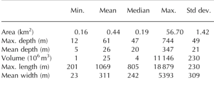
Area, depth and volume are key variables to quantify overdeepenings, and their calculation and interpretation are straightforward. However, for other morphometric proper-ties of overdeepenings (i.e. length and width), measurement approaches become more difficult to define (Patton and others, 2015). Statistics for some morphometric properties for the modelled overdeepenings are summarized in Table 1. Accordingly, a mean overdeepening in the HK region has an area of 0.44 km2 and a volume of 25 � 106m3 (note that these statistics are based on overdeepenings >106m3).
Half of the modelled overdeepenings (in terms of area and volume) are found in the Karakoram (Table 2). However, these make up only �5.4% of the glacierized area in the Karakoram, owing to the large overall area of glaciation. In the western Himalaya numerous large over-deepenings are also found, containing about a quarter of the region-wide total volume and comprising 4.5% of the western Himalaya glacierized area. In the central and eastern Himalaya the modelled volume of the overdeepen-ings is minor compared to the total ice volume, and the percentage of overdeepened area is smaller (3.5% for central, 3.9% for eastern Himalaya). Table 2 shows that for the Karakoram and central Himalaya, the ratio between overdeepened volume and total ice volume is smaller than the area ratio, whereas the opposite is true for the western and eastern Himalaya. This implies that the overdeepenings are generally deeper in the western and eastern Himalaya and shallower in the central Himalaya and Karakoram. By applying a 10 m freeboard some larger shallow parts of the overdeepenings are eliminated, resulting in higher absolute mean depths for the remaining overdeepenings (Table 2). 4.2. Test cases for sub-regions
The results for the four sub-regions are discussed based on the test areas defined earlier. The eastern and central Himalayan glaciers gain mass mainly during the Indian summer monsoon (these glaciers are hence called summer-accumulation type glaciers; Ageta and Higuchi, 1984), whereas winter accumulation is more important for the glaciers in the northwest (western Himalaya and Karakoram; Benn and Owen, 1998). The characteristics of the Hima-layan glaciers may therefore differ by sub-region. For each test region, ten larger overdeepenings were visually exam-ined using Google Earth with respect to the morphological indicator criteria defined by Frey and others (2010). One of
Table 1. Statistics for large overdeepenings (>106m3) for the entire
HK region as modelled with GlabTop2
Min. Mean Median Max. Std dev. Area (km2) 0.16 0.44 0.19 56.70 1.42 Max. depth (m) 12 61 47 744 49 Mean depth (m) 5 26 20 347 21 Volume (106m3) 1 25 4 11 146 230 Max. length (m) 201 1069 805 18 879 230 Mean width (m) 23 311 242 5393 309
Table 2. Modelled glacier thicknesses and overdeepenings (>106m3) for individual sub-regions. The area (volume) ratios give the percentage of the overdeepened area (volume) with respect to the area (volume) of the glaciers
Glaciers* Overdeepenings (>106m3)
Filled to top Leaving a 10 m freeboard Area Volume Area Area ratio Mean
depth
Volume Volume ratio
Area Area ratio Mean depth Volume Volume ratio km2 km3 km2 % m km3 % km2 % m km3 % Karakoram 17 946 1683 975 5.4 59 57 3.4 795 4.4 61 48 2.9 Western Himalaya 8943 504 402 4.5 82 33 6.6 276 3.1 88 24 4.8 Central Himalaya 9940 553 352 3.5 40 14 2.6 335 3.4 40 13 2.4 Eastern Himalaya 3946 215 154 3.9 77 12 5.5 126 3.2 83 10 4.8 Total HK region 40 775 2955 1883 4.6 2 116 3.9 1532 3.8 63 96 3.3
the chosen glaciers may be surging and four are heavily debris-covered and probably downwasting rather than retreating. All the remaining 35 examined overdeepenings are in crevasse-free areas indicating longitudinal compres-sion where ice flows over adverse bed slopes. Fourteen of these overdeepenings (40%) exhibit a slope increase or a transition to transverse crevasses in the flow direction, indicating flow acceleration over the down-valley side of a bedrock riegel combined with a lateral narrowing of the flow. Twelve (34%) fulfil all these aforementioned morpho-logical criteria as defined by Frey and others (2010). Despite general uncertainties in shape, the larger modelled features most probably reflect real bed overdeepenings. These generally correspond well with locations where glacier surface slope is <5°.
4.2.1. Karakoram
The gently sloping tongues of Siachen and Baltoro glaciers with surface slopes <5° are estimated to be up to 800 m thick. A number of overdeepenings are modelled under-neath this thick ice cover. Numerous overdeepenings are located at glacier confluences (red circles in Fig. 4). High-resolution satellite images from Google Earth reveal that some modelled depressions are just up-glacier of transverse crevasse patterns and increasing slope gradients which indicate extending flow over riegel structures in the bed (yellow rectangles in Fig. 4). The largest modelled over-deepening at central Rimo glacier, displayed in Figure 4 (lower right of the image), covers an area of >50 km2and has a volume of �11 km3. Some glacier tongues on the northern slope of the main ridge (green arrows in Fig. 4) have gently looped medial moraines, and the mapped
glacier outlines (from the first Chinese Glacier Inventory) notably exceed the ice cover visible in the Google Earth image. This may imply surge-type behaviour which makes prediction of bed overdeepenings problematic.
4.2.2. Western Himalaya
The erroneous void fillings within the western Himalaya SRTM DEM have an influence on the modelled geometry. As illustrated in Figure 5a, in mountainous terrain with steep slopes and associated data voids, many modelled depres-sions correspond closely with the filled voids (shadowed areas) in the DEM. Flatter glacier parts with continuous DEM data are not affected by these artefacts. For Chhota Shigri glacier, five GPR profiles are available (Azam and others, 2012), allowing us to compare measured and modelled ice thicknesses directly (Fig. 5b). The measured glacier surface elevations are generally lower than the SRTM DEM at the same locations. Therefore, for the comparison, the glacier surface from the SRTM and the associated modelled bed topography have been shifted to match the elevation of the GPR measurements at the surface. The model results generally capture well the geometries of the glacier cross sections. With the exception of profile 3, the modelled ice thicknesses seem to be underestimated, but the deviations between measurements and model outputs mostly remain within the model uncertainty range of �30%.
4.2.3. Central Himalaya
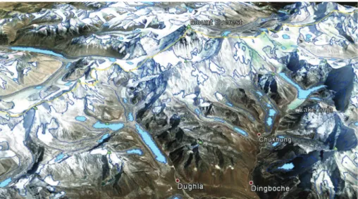
Recent glacier shrinkage has resulted in increasing debris cover of glaciers accompanied by continued formation and growth of pro- and supraglacial lakes (Bolch and others, 2008). The well-documented rapid expansion of Imja lake at
Fig. 4. Modelled bed overdeepenings (>106m3) for glaciers between K2 and the Karakoram Pass in the Karakoram Range including Siachen and Baltoro glaciers, the largest glaciers in the Himalaya Karakoram region. The light-blue outline shows the largest modelled depression at central Rimo glacier (lower right of image). Red circles show overdeepenings at glacier confluences, yellow rectangles show overdeepenings with following extending flow, and green arrows indicate (the direction of) surge-type glaciers.
Linsbauer and others: Possible future lakes in the Himalaya–Karakoram
the middle right of Figure 6 is of considerable concern. The model results are in agreement with recent GPR soundings by Somos-Valenzuela and others (2014). They showed that the lake can grow further towards the steep icy slopes of the surrounding high mountain flanks, which could be a problematic development as the stability of these slopes is likely to decrease due to glacier debuttressing and perma-frost degradation (Haeberli and others, in press).
4.2.4. Eastern Himalaya
Several of the northern, debris-free glaciers in the Bhutan Himalaya end in moraine-dammed lakes (Fig. 7). Because the glacier tongues are predominantly gently sloping and thick, there is potential for further lake enlargement as glaciers retreat further. In the accumulation area below the firn/ice plateaus where some of these glaciers originate, our model results indicate the presence of several subglacial
Fig. 5. (a) Modelled overdeepenings (blue) for a subscene of the western Himalaya at the Pir Panjal range (Chandra and Parbati valley,
Himachal Pradesh, India). The profiles with the GPR measurements at Chhota Shigri are shown in red, and the black rectangle refers to Chhota Shigri for (b). (b) Comparison of GPR measurements (five profiles) with modelled ice thicknesses of Chhota Shigri glacier. Elevation (m a.s.l.) and lateral distance (m) are plotted in y- and x-axis, respectively, for each cross section.
overdeepenings. This, however, is not seen in the accumu-lation areas of the steep south-orientated glaciers; in these cases overdeepenings are only modelled under flat and heavily debris-covered tongues. The mountain topography south of the main ridge shows numerous pre-existing glacial lakes (dark blue in Fig. 7). For the smaller glaciers present in this part of the scene, more potential future lakes are modelled.
5. DISCUSSION AND IMPLICATIONS 5.1. Data quality
In general we suggest that with higher data quality, particularly surface DEMs, the robustness of the modelled overdeepenings could be enhanced. Frey and Paul (2012) found that in glacier-covered terrain the SRTM DEM is
slightly superior to the first version of the photogrammetric ASTER GDEM. The main problem with the SRTM DEM in our study region is the erroneous void filling in the western Himalaya (Fig. 2a). As shown in Figure 5a, some modelled overdeepenings correspond closely with the filled voids of the SRTM DEM, and, as a consequence, some of these overdeepenings are very deep. This might partly explain why the overdeepenings in the western (and eastern) Himalaya are generally deeper than in the other regions (Table 2).
The quality of the glacier outlines used in this study is high for most parts of the HK region. Certainly there are some erroneous areas north of the Himalayan main range, where the glacier outlines are not accurate enough and could be improved (Fig 2b). For the employed method, this would affect the modelling of depressions in the glacier beds. In the case of Chhota Shigri, the comparison between
Fig. 6. Google Earth imagery of the region around Mount Everest, showing the glacier inventory (blue lines) and the modelled
overdeepenings (light blue).
Fig. 7. Modelled overdeepenings (green) for a glacier sample in the northernmost section of the Bhutan Himalayan main ridge. The
background picture is two Landsat scenes from 19 December 2000, showing the pre-existing proglacial lakes in dark blue.
Linsbauer and others: Possible future lakes in the Himalaya–Karakoram
model results and measurements in Figure 5b shows that the outlines used are somewhat larger than the glacier is in reality. However, this has no major influence on the modelling of overdeepenings.
5.2. Model choice and limitations
Different approaches for estimating ice thickness distribu-tions (e.g. Farinotti and others, 2009; Huss and Farinotti, 2012; Linsbauer and others, 2012; Clarke and others, 2013; Frey and others, 2014) could potentially be used to model the bed topography of glaciers, and a model comparison would be interesting, but should be done in a region with more measured data than are available in the HK region. As the aim of this study is to highlight the regional aspect in view of practical applications, we applied the GlabTop2 approach, which has the advantage of being simple and computationally efficient, requires minimal input data and has been validated with ice thickness measurements on HK glaciers (Frey and others, 2014). The direct comparison of GlabTop2 with the Huss and Farinotti (2012) approach, and with actual ice thickness measurements, revealed that the general pattern of the ice thickness distribution and the location of maximum ice thicknesses are similar in both models (Frey and others, 2014). Locally, large differences are observed between modelled and measured ice thick-ness; however, the deviations between measurements and both models are generally very similar.
General limits of GlabTop2 and comparable slope-related approaches, as mentioned before, concern the inability to capture effects of basal sliding or glacier surging. Other dynamic resistances (e.g. valley side drag) are only crudely accounted for and the constant shear stress assump-tion definitely breaks down at firn divides and at culmina-tions of ice caps. More specifically, the resistance associated with longitudinal stress gradients is more pronounced in glaciers with large overdeepenings (Adhikari and Marshall, 2013). The corresponding deviations from an assumed constant basal drag along the entire glacier, however, appear to be limited.
5.3. Debris-covered glaciers
Many glaciers in the studied region, particularly in the central Himalaya, have heavily debris-covered tongues (Scherler and others, 2011). Numerous proglacial lakes have already formed in such situations, especially where surface slopes <2° coincide with thickness losses >60 m since the Little Ice Age (Sakai and Fujita, 2010).
A thick cover of debris at glacier surfaces strongly reduces ablation (Banerjee and Shankar, 2013). Local mass-balance gradients can become very low or even negative on such glaciers. Typical dynamic response times of decades for clean mountain glaciers (Haeberli and Hoelzle, 1995) can be centuries for glaciers with flat debris-covered tongues (Jouvet and others, 2011). Debris-covered glacier tongues are indeed likely to be far out of equilibrium today. Their surface slopes can become ex-tremely small, and basal shear stresses can be corres-pondingly reduced to low or even near-zero values. An assumption of constant shear stresses throughout individual glaciers as used in our model may therefore overestimate glacier thickness and underestimate glacier-bed elevation for debris-covered glacier tongues.
Heavily debris-covered glaciers generally have thick sedimentary rather than rocky glacier beds (Haeberli,
1996; Zemp and others, 2005). Morainic material tends to smooth topographic irregularities at glacier beds. Unfortu-nately, our model does not capture this mechanism. The uncertainty of overdeepening geometries modelled for beds of debris-covered glaciers may therefore be quite high. Several overdeepenings modelled for some heavily debris-covered and downwasting glacier tongues, for instance, may primarily reflect irregularities in surface slope and could eventually turn into outwash plains rather than lakes.
Future proglacial lakes may start forming on the surfaces of debris-covered glaciers. As a useful empirical rule, a surface slope of �2° or lower enables the development of supraglacial lakes (Reynolds, 2000) as it corresponds well with zones of near-stagnant ice flow (Quincey and others, 2007). The larger glacier-bed overdeepenings modelled in the present study coincide with local surface slopes of �7° or less. The possibility of supraglacial lake formation is therefore included in this ad hoc approach. Debris-covered glaciers develop in catchments with especially high debris input from surrounding rock walls. Such an elevated sediment flux may lead to rapid infilling of overdeepenings and to a reduction in the lifetime of future proglacial lakes. The latter depends on the ratio between the lake volume and the input rate of sediments, which depends on catchment size and erosion rates. Erosion rates in cold mountain ranges vary over orders of magnitude (Hallet and others, 1996; Delmas and others, 2009; Koppes and Montgomery, 2009) and can increase by an order of magnitude in the case of strong deglaciation and permafrost degradation, prior to slope stabilization by re-vegetation (Hinderer, 2001; Fischer and others, 2013). With characteristic erosion rates of 1– 10 mm a–1 for conditions of rapid warming assumed here, many of the modelled lakes (if formed) can easily attain lifetimes of 102–103years even with high debris inputs. 5.4. Glacial lake outburst hazard
In terms of the hazard associated with future lake develop-ment in the HK region, it is notable that the mean areal extent of modelled overdeepenings (�0.44 km2) is consider-ably larger (by a factor of 5) than mean values currently observed for glacial lakes across the Indian Himalaya (Worni and others, 2013), Nepal (ICIMOD, 2011) or the wider Hindu Kush–Himalayan region (Ives and others, 2010). While this reflects the focus of the current study on largest overdeepenings (>106m3), it also gives an insight into the magnitude of potential future lake outbursts. Given the currently observed rapid expansion of proglacial lakes in the region, and the expected large size of new lakes forming in the future, approaches to manage and reduce the risk of future lake outburst hazard must anticipate and prepare for potentially very large-magnitude events. Currently, the largest-volume and most rapidly expanding glacial lakes are observed in the eastern areas of the Himalaya, particu-larly eastern Nepal and Bhutan (Gardelle and others, 2011; Fujita and others, 2013). Yet modelling of overdeepenings indicates that in an environment with a strongly reduced ice extent, the largest glacial lakes will be found in the western Himalaya and Karakoram. Hence, continued deglaciation of the HK region may imply a shift in the regional distribution of hazards associated with glacial lake outburst events.
6. CONCLUSION
Beneath the glacierized area (40 775 km2) of the HK region �16 000 bed overdeepenings have been modelled using the GlabTop2 approach for slope-related calculation of high-resolution glacier-bed topography. The modelled features exceeding 104m2in surface area cover �2200 km2(�5% of the currently glacierized area) and have a total volume of �120 km3(3–4% of the current glacier volume). Given the limitations in model parameterizations and input data, it is challenging to estimate the shapes of the overdeepenings accurately. However, their future appearance under the condition of continued glacier retreat, and also their locations, appear to be robust and can be confirmed by visual inspection of morphological criteria using satellite imagery. For debris-covered glaciers, ice-depth estimates may be much more uncertain and lifetimes of possible future lakes may likely be limited by high rates of sediment delivery from their catchments. Nevertheless, the presented information constitutes an important knowledge basis for assessing the potential risks and opportunities associated with the future proglacial lakes.
ACKNOWLEDGEMENTS
This study was funded by the Swiss Agency for Develop-ment and Cooperation (SDC) Indian Himalayas Climate Adaptation Programme (IHCAP: http://ihcap.in/) and the National Cooperative for the Disposal of Radioactive Waste (Nagra) in Switzerland within the framework of studies on glacial overdeepenings. We acknowledge the constructive reviews provided by two anonymous reviewers, which resulted in significant improvements to our manuscript, and the work of the Scientific Editor Surendra Adhikari and Chief Editor Graham Cogley.
REFERENCES
Adhikari S and Marshall SJ (2013) Influence of high-order mech-anics on simulation of glacier response to climate change: insights from Haig Glacier, Canadian Rocky Mountains.
Cryo-sphere, 7(5), 1527–1541 (doi: 10.5194/tc-7-1527-2013)
Ageta Y and Higuchi K (1984) Estimation of mass balance components of a summer-accumulation type glacier in the Nepal Himalaya. Geogr. Ann. A, 66(3), 249–255 (doi: 10.2307/ 520698)
Azam MF and 10 others (2012) From balance to imbalance: a shift in the dynamic behaviour of Chhota Shigri glacier, western Himalaya, India. J. Glaciol., 58(208), 315–324 (doi: 10.3189/ 2012JoG11J123)
Azam MF, Wagnon P, Vincent C, Ramanathan A, Linda A and Singh VB (2014) Reconstruction of the annual mass balance of Chhota Shigri glacier, Western Himalaya, India, since 1969.
Ann. Glaciol., 55(66), 69–80 (doi: 10.3189/2014AoG66A104)
Bajracharya SR and Mool P (2010) Glaciers, glacial lakes and glacial lake outburst floods in the Mount Everest region, Nepal. Ann.
Glaciol. 50(53), 81–86 (doi: 10.3189/172756410790595895)
Bajracharya SR and Shrestha B (2011) The status of glaciers in the
Hindu Kush–Himalayan region. International Centre for
Inte-grated Mountain Development, Kathmandu
Banerjee A and Shankar R (2013) On the response of Himalayan glaciers to climate change. J. Glaciol. 59(215), 480–490 (doi: 10.3189/2013JoG12J130)
Barrand NE and Murray T (2006) Multivariate controls on the incidence of glacier surging in the Karakoram Himalaya. Arct.
Antarct. Alp. Res., 38(4), 489–498 (doi: 10.1657/1523-0430
(2006)38[489:MCOTIO]2.0.CO;2)
Benn DI and Owen LA (1998) The role of the Indian summer monsoon and the mid-latitude westerlies in Himalayan glaci-ation: review and speculative discussion. J. Geol. Soc., 155(2), 353–363 (doi: 10.1144/gsjgs.155.2.0353)
Berthier E, Arnaud Y, Kumar R, Ahmad S, Wagnon P and Chevallier P (2007) Remote sensing estimates of glacier mass balances in the Himachal Pradesh (Western Himalaya, India). Remote Sens.
Environ., 108(3), 327–338 (doi: 10.1016/j.rse.2006.11.017)
Bhambri R, Bolch T, Kawishwar P, Dobhal DP, Srivastava D and Pratap B (2013) Heterogeneity in glacier response in the upper Shyok valley, northeast Karakoram. Cryosphere, 7(5), 1385–1398 (doi: 10.5194/tc-7-1385-2013)
Binder D, Brückl E, Roch KH, Behm M, Schöner W and Hynek B (2009) Determination of total ice volume and ice-thickness distribution of two glaciers in the Hohe Tauern region, Eastern Alps, from GPR data. Ann. Glaciol., 50(51), 71–79
Bolch T, Buchroithner M, Pieczonka T and Kunert A (2008) Planimetric and volumetric glacier changes in the Khumbu Himal, Nepal, since 1962 using Corona, Landsat TM and ASTER data. J. Glaciol., 54(187), 592–600 (doi: 10.3189/ 002214308786570782)
Bolch T and 11 others (2012) The state and fate of Himalayan glaciers. Science, 336(6079), 310–314 (doi: 10.1126/science. 1215828)
Bookhagen B and Burbank DW (2006) Topography, relief, and TRMM-derived rainfall variations along the Himalaya. Geophys.
Res. Lett., 33(8), L08405 (doi: 10.1029/2006GL026037)
Bookhagen B and Burbank DW (2010) Toward a complete Hima-layan hydrological budget: spatiotemporal distribution of snow-melt and rainfall and their impact on river discharge. J. Geophys.
Res.: Earth Surf., 115(F3), F03019 (doi: 10.1029/2009JF001426)
Chikita K, Joshi SP, Jha J and Hasegawa H (2000) Hydrological and thermal regimes in a supra-glacial lake: Imja, Khumbu, Nepal Himalaya. Hydrol. Sci. J., 45(4), 507–521 (doi: 10.1080/ 02626660009492353)
Clarke GKC, Berthier E, Schoof CG and Jarosch AH (2009) Neural networks applied to estimating subglacial topography and glacier volume. J. Climate, 22(9), 2146–2160 (doi: 10.1175/ 2008JCLI2572.1)
Clarke GKC and 6 others (2013) Ice volume and subglacial topography for western Canadian glaciers from mass balance fields, thinning rates, and a bed stress model. J. Climate, 26(12), 4282–4303 (doi: 10.1175/JCLI-D-12-00513.1)
Cook SJ and Swift DA (2012) Subglacial basins: their origin and importance in glacial systems and landscapes. Earth-Sci. Rev.,
115(4), 332–372 (doi: 10.1016/j.earscirev.2012.09.009)
Delmas M, Calvet M and Gunnell Y (2009) Variability of Quater-nary glacial erosion rates: a global perspective with special reference to the Eastern Pyrenees. Quat. Sci. Rev., 28(5–6), 484–498 (doi: 10.1016/j.quascirev.2008.11.006)
Environmental Systems Research Institute (ESRI) (2011) ArcGIS
Desktop: Release 10. Environmental Systems Research Institute,
Redlands, CA
Farinotti D, Huss M, Bauder A and Funk M (2009) An estimate of the glacier ice volume in the Swiss Alps. Global Planet. Change
68(3), 225–231 (doi: 10.1016/j.gloplacha.2009.05.004)
Farr TG and 17 others (2007) The Shuttle Radar Topography Mission. Rev. Geophys., 45(2) (doi: 10.1029/2005RG000183) Fischer L, Huggel C, Kääb A and Haeberli W (2013) Slope failures
and erosion rates on a glacierized high-mountain face under climatic changes. Earth Surf. Process. Landf., 38(8), 836–846 (doi: 10.1002/esp.3355)
Frey H and Paul F (2012) On the suitability of the SRTM DEM and ASTER GDEM for the compilation of topographic parameters in glacier inventories. Int. J. Appl. Earth Obs. Geoinf., 18, 480–490 (doi: 10.1016/j.jag.2011.09.020)
Frey H, Haeberli W, Linsbauer A, Huggel C and Paul F (2010) A multi-level strategy for anticipating future glacier lake formation and associated hazard potentials. Natur. Hazards Earth Syst.
Sci., 10(2), 339–352
Linsbauer and others: Possible future lakes in the Himalaya–Karakoram
Frey H, Paul F and Strozzi T (2012) Compilation of a glacier inventory for the western Himalayas from satellite data: methods, challenges, and results. Remote Sens. Environ., 124, 832–843 (doi: 10.1016/j.rse.2012.06.020)
Frey H, and 9 others (2014) Estimating the volume of glaciers in the Himalayan–Karakoram region using different methods.
Cryo-sphere, 8(6), 2313–2333 (doi: 10.5194/tc-8-2313-2014)
Fujita K, Sakai A, Nuimura T, Yamaguchi S and Sharma RR (2009) Recent changes in Imja Glacial Lake and its damming moraine in the Nepal Himalaya revealed by in situ surveys and multi-temporal ASTER imagery. Environ. Res. Lett., 4(4), 045205 (doi: 10.1088/1748-9326/4/4/045205)
Fujita K and 6 others (2013) Potential flood volume of Himalayan glacial lakes. Natur. Hazards Earth Syst. Sci., 13(7), 1827–1839 (doi: 10.5194/nhess-13-1827-2013)
Gardelle J, Arnaud Y and Berthier E (2011) Contrasted evolution of glacial lakes along the Hindu Kush Himalaya mountain range between 1990 and 2009. Global Planet. Change, 75(1–2), 47–55 (doi: 10.1016/j.gloplacha.2010.10.003)
Giesen RH and Oerlemans J (2010) Response of the ice cap Hardangerjøkulen in southern Norway to the 20th and 21st century climates. Cryosphere, 4(2), 191–213 (doi: 10.5194/tc-4-191-2010)
Gurung H (1999) Mountains of Asia. International Centre for Integrated Mountain Development, Kathmandu
Haeberli W (1996) On the morphodynamics of ice/debris-transport systems in cold mountain areas. Nor. Geogr. Tidsskr., 50(1), 3–9 (doi: 10.1080/00291959608552346)
Haeberli W and Hoelzle M (1995) Application of inventory data for estimating characteristics of and regional climate-change effects on mountain glaciers: a pilot study with the European Alps. Ann.
Glaciol., 21, 206–212
Haeberli W and Linsbauer A (2013) Brief Communication. Global glacier volumes and sea level: small but systematic effects of ice below the surface of the ocean and of new local lakes on land.
Cryosphere, 7(3), 817–821 (doi: 10.5194/tc-7-817-2013)
Haeberli W and Schweizer J (1988) Rhonegletscher 1850: Eismechanische Ueberlegungen zu einem historischen Gletscherstand. Mitt. VAW ETHZ, 94, 59–70
Haeberli W, Schaub Y and Huggel C (in press) Increasing risks related to landslides from degrading permafrost into new lakes in de-glaciating mountain ranges. Geomorphology
Hallet B, Hunter L and Bogen J (1996) Rates of erosion and sediment evacuation by glaciers: a review of field data and their implications. Global Planet. Change, 12(1–4), 213–235 (doi: 10.1016/0921-8181(95)00021-6)
Hinderer M (2001) Late Quaternary denudation of the Alps, valley and lake fillings and modern river loads. Geodin. Acta, 13, 1778–1786
Hooke RLeB (1991) Positive feedbacks associated with erosion of glacial cirques and overdeepenings. Geol. Soc. Am. Bull.,
103(8), 1104–1108 (doi: 10.1130/0016-7606(1991)103<1104:
PFAWEO>2.3.CO;2)
Huss M and Farinotti D (2012) Distributed ice thickness and volume of all glaciers around the globe. J. Geophys. Res.,
117(F4), F04010 (doi: 10.1029/2012JF002523)
Immerzeel W, Van Beek L, Konz M, Shrestha A and Bierkens M (2012) Hydrological response to climate change in a glacierized catchment in the Himalayas. Climate Change, 110(3), 721–736 (doi: 10.1007/s10584-011-0143-4)
International Centre for Integrated Mountain Development (ICI-MOD) (2011) Glacial lakes and glacial lake outburst floods in
Nepal. International Centre for Integrated Mountain
Develop-ment, Kathmandu http://lib.icimod.org/record/27755
Ives JD, Shrestha RB and Mool PK (2010) Formation of glacial lakes
in the Hindu Kush–Himalayas and GLOF risk assessment.
International Centre for Integrated Mountain Development, Kathmandu http://lib.icimod.org/record/8047
Jouvet G, Huss M, Funk M and Blatter H (2011) Modelling the retreat of Grosser Aletschgletscher, Switzerland, in a changing
climate. J. Glaciol., 57(206), 1033–1045 (doi: 10.3189/ 002214311798843359)
Kääb A (2005) Combination of SRTM3 and repeat ASTER data for deriving alpine glacier flow velocities in the Bhutan Himalaya.
Remote Sens. Environ., 94(4), 463–474 (doi: 10.1016/j.rse.
2004.11.003)
Koppes MN and Montgomery DR (2009) The relative efficacy of fluvial and glacial erosion over modern to orogenic timescales.
Nature Geosci., 2(9), 644–647 (doi: 10.1038/ngeo616)
Künzler M, Huggel C, Linsbauer A and Haeberli W (2010) Emerging risks related to new lakes in deglaciating areas of the Alps. In Malet J-P, Glade T and Casagli N eds Mountain
Risks: Bringing Science to Society. Proceedings of the ‘Mountain Risk’ International Conference, 24–26 November 2010, Firenze, Italy. CERG Editions, Strasbourg, 453–458
Li H, Ng Z, Li F, Qin D and Cheng G (2012) An extended ‘perfect-plasticity’ method for estimating ice thickness along the flow line of mountain glaciers. J. Geophys. Res., 117(F1), F01020 (doi: 10.1029/2011JF002104)
Linsbauer A, Paul F, Hoelzle M, Frey H and Haeberli W (2009) The Swiss Alps without glaciers: a GIS-based modelling approach for reconstruction of glacier beds. In Purves R, Gruber S, Straumann R and Hengl T eds Proceedings of Geomorphometry 2009. University of Zürich, Zürich, 243–247 http://www.geomorpho-metry.org/linsbauer2009geomorphometry
Linsbauer A, Paul F and Haeberli W (2012) Modeling glacier thickness distribution and bed topography over entire mountain ranges with GlabTop: application of a fast and robust approach. J. Geophys. Res., 117(F3), F03007 (doi: 10.1029/ 2011JF002313)
Loriaux T and Casassa G (2013) Evolution of glacial lakes from the Northern Patagonia Icefield and terrestrial water storage in a sea-level rise context. Global Planet. Change, 102, 33–40 (doi: 10.1016/j.gloplacha.2012.12.012)
Marshall S and 7 others (2011) Glacier water resources on the eastern slopes of the Canadian Rocky Mountains. Can. Water
Resour. J., 36(2), 109–134 (doi: 10.4296/cwrj3602823)
Patton H, Swift DA, Clark CD, Livingstone SJ, Cook SJ and Hubbard A (2015) Automated mapping of glacial overdeepenings beneath contemporary ice sheets: approaches and potential applications. Geomorphology, 232, 209–223 (doi: 10.1016/j. geomorph.2015.01.003)
Paul F and Linsbauer A (2012) Modeling of glacier bed topography from glacier outlines, central branch lines, and a DEM.
Int. J. Geogr. Inf. Sci., 26(7), 1173–1190 (doi: 10.1080/
13658816.2011.627859)
Pfeffer WT and 75 others (2014) The Randolph Glacier Inventory: a globally complete inventory of glaciers. J. Glaciol., 60(221), 537–552 (doi: 10.3189/2014JoG13J176)
Quincey DJ and 6 others (2007) Early recognition of glacial lake hazards in the Himalaya using remote sensing datasets. Global
Planet. Change, 56(1–2), 137–152 (doi: 10.1016/j.gloplacha.
2006.07.013)
Rankl M, Kienholz C and Braun M (2014) Glacier changes in the Karakoram region mapped by multimission satellite imagery. Cryosphere, 8(3), 977–989 (doi: 10.5194/tc-8-977-2014)
Reuter HI, Nelson A and Jarvis A (2007) An evaluation of void-filling interpolation methods for SRTM – data. Int. J. Geogr. Inf.
Sci., 21(9), 983 (doi: 10.1080/13658810601169899)
Reynolds JM (2000) On the formation of supraglacial lakes on debris-covered glaciers. IAHS Publ. 264 (Workshop at Seattle 2000 – Debris-Covered Glaciers), 153–161
Sakai A and Fujita K (2010) Formation conditions of supraglacial lakes on debris-covered glaciers in the Himalaya. J. Glaciol.
56(195), 177–181 (doi: 10.3189/002214310791190785)
Schaub Y, Haeberli W, Huggel C, Künzler M and Bründl M (2013) Landslides and new lakes in deglaciating areas: a risk manage-ment framework. In Margottini C, Canuti P and Sassa K eds
31–38 http://link.springer.com/chapter/10.1007/978-3-642-31313-4_5
Scherler D, Bookhagen B and Strecker MR (2011) Spatially variable response of Himalayan glaciers to climate change affected by debris cover. Nature Geosci., 4(3), 156–159 (doi: 10.1038/ ngeo1068)
Shi Y, Liu C and Kang E (2010) The Glacier Inventory of China.
Ann. Glaciol. 50(53), 1–4 (doi: 10.3189/172756410790595831)
Shroder JF (2011) Himalaya. In Singh VP, Singh P and Haritashya UK eds Encyclopedia of snow, ice, and glaciers. Springer Science + Business Media, Dordrecht, 510–520
Somos-Valenzuela MA, McKinney DC, Rounce DR and Byers AC (2014) Changes in Imja Tsho in the Mount Everest region of Nepal. Cryosphere 8(5), 1661–1671 (doi: 10.5194/tc-8-1661-2014)
Terrier S, Jordan F, Schleiss AJ, Haeberli W, Huggel C and Künzler M (2011) Optimized and adapted hydropower management con-sidering glacier shrinkage scenarios in the Swiss Alps. In Schleiss A and Boes RM eds Proceedings of the International Symposium
on Dams and Reservoirs under Changing Challenges – 79th Annual Meeting of ICOLD, Swiss Committee on Dams, Lucerne, Switzerland. Taylor & Francis, London, 497–508
Wagnon P and 10 others (2007) Four years of mass balance on Chhota Shigri Glacier, Himachal Pradesh, India, a new benchmark glacier in the western Himalaya. J. Glaciol.,
53(183), 603–611 (doi: 10.3189/002214307784409306)
Worni R, Huggel C and Stoffel M (2013) Glacial lakes in the Indian Himalayas: from an area-wide glacial lake inventory to on-site and modeling based risk assessment of critical glacial lakes. Sci.
Total Environ., 468–469(Suppl.), 71–84 (doi:
10.1016/j.scito-tenv.2012.11.043)
Yamada T and Sharma CK (1993) Glacier lakes and outburst floods in the Nepal Himalaya. IAHS Publ. 218 (Symposium at Kathmandu 1992 – Snow and Glacier Hydrology), 319–330 Zekollari H, Huybrechts P, Fürst JJ, Rybak O and Eisen O (2013)
Calibration of a higher-order 3-D ice-flow model of the Morteratsch glacier complex, Engadin, Switzerland. Ann.
Glaciol., 54(63), 343–351 (doi: 10.3189/2013AoG63A434)
Zekollari H, Fürst JJ and Huybrechts P (2015) Modelling the evolution of Vadret da Morteratsch, Switzerland, since the Little Ice Age and into the future. J. Glaciol., 60(224), 1155–1168 Zemp M, Kääb A, Hoelzle M and Haeberli W (2005) GIS-based
modelling of glacial sediment balance. Z. Geomorphol., 138, 113–129
Linsbauer and others: Possible future lakes in the Himalaya–Karakoram