Atlantic Ocean Circulation at the Last Glacial Maximum:
Inferences from Data and Models
by
Holly Janine Dail
Submitted in partial fulfillment of the requirements for the degree of
Doctor of Philosophy
at the
MASSACHUSETTS INSTITUTE OF TECHNOLOGY
and the
WOODS HOLE OCEANOGRAPHIC INSTITUTION
September 2012
c
Holly Janine Dail, MMXII. All rights reserved.
The author hereby grants to MIT and WHOI permission to reproduce and
to distribute publicly paper and electronic copies of this thesis document in
whole or in part in any medium now known or hereafter created.
Signature of Author . . . .
Joint Program in Oceanography – Massachusetts Institute of Technology /
Woods Hole Oceanographic Institution
August 14, 2012
Certified by . . . .
Carl I. Wunsch
Cecil and Ida Green Professor of Physical Oceanography
Massachusetts Institute of Technology
Thesis Supervisor
Accepted by . . . .
Karl R. Helfrich
Senior Scientist, Woods Hole Oceanographic Institution
Atlantic Ocean Circulation at the Last Glacial Maximum:
Inferences from Data and Models
by
Holly Janine Dail
Submitted to the Joint Program in Oceanography,
Massachusetts Institute of Technology and the Woods Hole Oceanographic Institution on August 14, 2012, in partial fulfillment of the requirements for the degree of
Doctor of Philosophy
Abstract
This thesis focuses on ocean circulation and atmospheric forcing in the Atlantic Ocean at the Last Glacial Maximum (LGM, 18-21 thousand years before present). Relative to the pre-industrial climate, LGM atmospheric CO2 concentrations were about 90 ppm lower, ice sheets were much more extensive, and many regions experienced significantly colder temperatures. In this thesis a novel approach to dynamical reconstruction is applied to make estimates of LGM Atlantic Ocean state that are consistent with these proxy records and with known ocean dynamics.
Ocean dynamics are described with the MIT General Circulation Model in an Atlantic configuration extending from 35◦S to 75◦N at 1◦ resolution. Six LGM proxy types are used to constrain the model: four compilations of near sea surface temperatures from the MARGO project, as well as benthic isotope records ofδ18
O andδ13
C compiled by Marchal and Curry; 629 individual proxy records are used. To improve the fit of the model to the data, a least-squares fit is computed using an algorithm based on the model adjoint (the Lagrange multiplier methodology). The adjoint is used to compute improvements to uncertain initial and boundary conditions (the control variables). As compared to previous model-data syntheses of LGM ocean state, this thesis uses a significantly more realistic model of oceanic physics, and is the first to incorporate such a large number and diversity of proxy records.
A major finding is that it is possible to find an ocean state that is consistent with all six LGM proxy compilations and with known ocean dynamics, given reasonable uncertainty estimates. Only relatively modest shifts from modern atmospheric forcing are required to fit the LGM data. The estimates presented herein succesfully reproduce regional shifts in conditions at the LGM that have been inferred from proxy records, but which have not been captured in the best available LGM coupled model simulations. In addition, LGM benthic
δ18
O andδ13
C records are shown to be consistent with a shallow but robust Atlantic merid-ional overturning cell, although other circulations cannot be excluded.
Thesis Supervisor: Carl I. Wunsch
Acknowledgments
First, I thank Carl Wunsch, my advisor. Carl has impeccable taste in choosing scientific problems, and the wisdom, perspective, and fortitude to make meaningful contributions to even the most difficult. I have benefited greatly from his patient guidance and clear vision. My thesis committee has been invaluable. Patrick Heimbach was incredibly helpful throughout with both adjoint modeling and with modern oceanography; I owe him much. Olivier Marchal graciously shared his extensive knowledge about proxy records and helped define appropriate assumptions for modeling isotopes. From Peter Huybers I have learned much about how to frame a problem effectively, and how to reduce it to its simplest form. Finally, Jake Gebbie has generously shared his wisdom from extensive experience with nearly all the subjects addressed in the thesis, and provided much needed advice at critical stages.
Many useful contributions have been made to this work from other collaborators. In the ECCO group, Ga¨el Forget’s state estimation expertise has been of great value, and early help from Constantinos Evangelinos is appreciated. Jean-Michel Campin has been patient, gracious with his time, and wonderfully helpful. Dan Amrhein generously read an earlier version of the thesis and provided many helpful comments. I also thank Delia Oppo, Bill Curry, Andr´e Paul, Martin Losch, Bette Otto-Bliesner, Nan Rosenbloom, and Esther Brady. The Academic Programs Office at WHOI and the administrative staff at MIT have been a great resource and have provided a human face to the program. I especially thank Marsha Armando, Julia Westwater, Annie Doucette, Beth MacEachran, and Mary Elliff.
Classes and generals would have been much less fun and a lot more challenging without Pat, Rachel, Rebecca, Cim, Laura, and Ryan. Early office mates Stephanie, Yohai, and Matt were, and continue to be, great mentors. Brian, Jinbo, Martha, and Sophie C. have been great colleagues too.
Finishing this thesis involved some dark days and I am grateful to my friends and family who supported me through it all. I especially thank my parents and my sister who supported me, as always, through thick and thin. I also owe thanks to friends Kate, Leeann, Kathy, Margaret, Shaun, Debbie, and Kurt.
I dedicate this thesis to my family – to my husband Alan, who is an incredible partner, and to Norah, who is very patiently teaching us what is truly important.
Financial support. I gratefully acknowledge the following financial support. Primary
support was provided by a National Defense Science and Engineering Graduate Fellow-ship and two National Science Foundation awards: Award #OCE-0645936: “Beyond the Instrumental Record: the Case of Circulation at the Last Glacial Maximum” and Award #OCE-1060735: “Collaborative Research: Beyond the Instrumental Record - the Ocean Circulation at the Last Glacial Maximum and the de-Glacial Sequence”. Important sec-ondary support came from the National Ocean Partnership Program and the National Aero-nautics and Space Administration via the ECCO effort at MIT.
Computational resources. This work required significant computer time. Preliminary
work relied on resources at NCAR, on local resources in the ECCO group at MIT, and on the “Swell” departmental cluster at Harvard. The final results were all computed on the Na-tional Aeronautics and Space Administration Pleiades machine under the ECCO2 project allocation. This is the most professionally run compute resource I have used in 15 years of parallel computing.
Providers of data and model output. I acknowledge the members of the MARGO
project for providing reconstructed LGM SST and sea ice estimates; O. Marchal and W. Curry for providing LGM and Holocene benthic isotope data; the PMIP2 international modeling groups for providing their model output for analysis; the Laboratoire des Sci-ences du Climat et de l’Environnement for collecting and archiving the PMIP2 output; W.R. Peltier for providing ICE-5G bathymetry and coastline estimates; A. LeGrande and G. Schmidt for providing a modern database ofδ18
Owatermeasurements; and the GEOSECS
project for making available modern water columnδ13
Abbreviated Contents
List of Figures 13
List of Tables 17
Acronyms used in the thesis 19
1 Introduction 21
2 Last Glacial Maximum Atlantic 31
3 State estimation methodology with application to modern circulation 85
4 Upper ocean conditions at the Last Glacial Maximum 145
5 Deep ocean conditions at the Last Glacial Maximum 191
6 Discussion 209
A MARGO uncertainty assignments 217
Contents
List of Figures 13
List of Tables 17
Acronyms used in the thesis 19
1 Introduction 21
1.1 The Last Glacial Maximum . . . 22
1.2 Dynamical reconstruction . . . 24
1.3 Terminology . . . 27
1.4 Structure of the thesis . . . 28
2 Last Glacial Maximum Atlantic 31 2.1 Geography and atmospheric State . . . 32
2.2 Proxies of LGM ocean state . . . 38
2.2.1 Introduction to potential uncertainties and biases . . . 39
2.2.2 Upper ocean state . . . 42
2.2.3 Deep ocean state . . . 54
2.3 Forward models of ocean state . . . 70
2.3.1 The Paleoclimate Modeling Intercomparison Project . . . 71
2.3.2 Isotope models . . . 74
2.4.1 Quantitative model-data comparison . . . 80
2.4.2 Synthesizing models and data . . . 81
2.5 Selection of data constraints for the thesis . . . 84
2.6 Chapter summary . . . 84
3 State estimation methodology with application to modern circulation 85 3.1 Forward model configuration . . . 86
3.1.1 Numerics and domain . . . 86
3.1.2 Initial and boundary conditions . . . 89
3.2 Ocean state estimation . . . 90
3.2.1 A least-squares problem and the method of Lagrange multipliers . . 91
3.2.2 Data constraints and uncertainties . . . 96
3.2.3 Control variables and uncertainties . . . 98
3.2.4 A focus on equilibrium ocean estimation . . . 101
3.3 State estimation with modern T/S information: the Modern TS estimate . . 102
3.3.1 Cost reduction . . . 102
3.3.2 Consistency of the state estimate . . . 104
3.3.3 Inferred properties . . . 112
3.4 Modern state estimation withδ13 CDICandδ 18 Owater observations . . . 117
3.4.1 δ18 Owater: forward modeling and state estimation . . . 119
3.4.2 δ13 CDIC: forward modeling and state estimation . . . 122
3.4.3 The Modern Iso estimate . . . 126
3.5 Extending state estimate length: the search for a seasonal steady state . . . 129
3.5.1 Asynchronous timestepping . . . 129
3.5.2 Carry-over control . . . 133
3.5.3 Analysis of a longer state estimate: Modern 80yrs . . . 135
3.5.4 Current limitations in equilibrium ocean estimation . . . 142
4 Upper ocean conditions at the Last Glacial Maximum 145
4.1 Forward model . . . 147
4.1.1 First guess initial conditions . . . 148
4.1.2 First guess atmospheric forcing . . . 149
4.2 Adjoint model . . . 150
4.3 Exploration of assumptions . . . 152
4.3.1 Using all MARGO data as published: LGM AllSSTs . . . 153
4.3.2 Using subsets of data: LGM NoForams and LGM Forams . . . 156
4.3.3 Using larger atmospheric uncertainties: LGM ForamsX2 . . . 158
4.4 A best estimate: LGM Upper . . . 158
4.4.1 Assumptions . . . 159
4.4.2 Consistency of the state estimate . . . 161
4.4.3 Analysis of solution . . . 167
4.5 Comparison to PMIP2 models . . . 176
4.5.1 Near sea surface temperatures . . . 176
4.5.2 Seasonality . . . 181
4.5.3 Wind field . . . 181
4.5.4 Sea ice distributions . . . 185
4.6 Chapter summary . . . 186
5 Deep ocean conditions at the Last Glacial Maximum 191 5.1 δ18 O andδ13 C data from benthic foraminifera . . . 192
5.2 Forward model and state estimation configuration . . . 193
5.3 The search for an acceptable solution . . . 195
5.4 Analysis of LGM Deep10yr and LGM Deep . . . 196
5.4.1 NSSTs and the MOC . . . 196
5.4.2 Modeled versus observedδ13 C . . . 200
5.4.3 Modeled versus observedδ18 O . . . 203
5.6 Chapter summary . . . 208
6 Discussion 209
6.1 A vision for ocean state estimation and equilibrium ocean estimation . . . . 209 6.2 Novel contributions of the thesis . . . 211 6.3 Limitations and opportunities for future progress . . . 212 6.4 Closing . . . 215
A MARGO uncertainty assignments 217
List of Figures
2-1 LGM coastlines, ice sheets, and temperatures (from Braconnot et al. 2012) . 33 2-2 ICE-4G and ICE-5G reconstructions of Laurentide ice sheet (from Li and
Battisti 2008) . . . 33
2-3 Maps of modern-LGM NSST differences (WOA’09 - MARGO) . . . 46
2-4 NSST differences (WOA’09 - MARGO) plotted against latitude . . . 47
2-5 LGM sea ice distributions (after De Vernal et al. 2006) . . . 52
2-6 LGM benthicδ18 Ocalciteandδ 13 Ccalcite proxy records with core depths . . . . 57
2-7 LGM pore-fluid measurements . . . 63
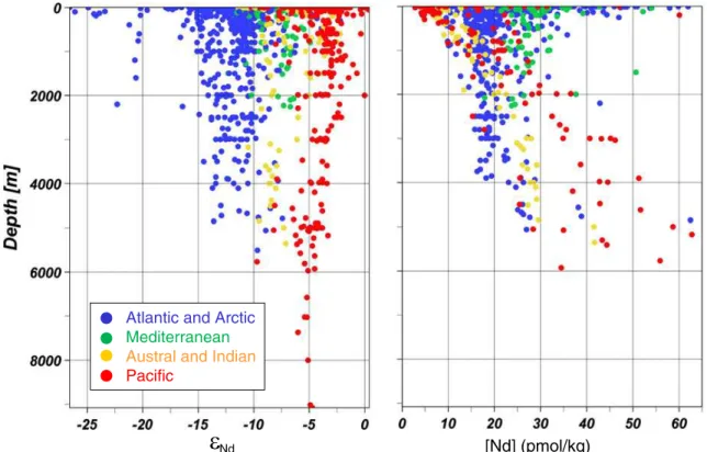
2-8 ModernǫNdand neodymium concentration (after Lacan et al. 2012) . . . . 64
2-9 Atlantic distributions of inferred Holocene and LGM seawater cadmium (from Marchitto and Broecker 2006) . . . 67
2-10 Scatter plots of modeled vs. observed LGMδ13 C (after Hesse et al. 2011) . 78 3-1 Evolution of data and control costs over 26 iterations . . . 103
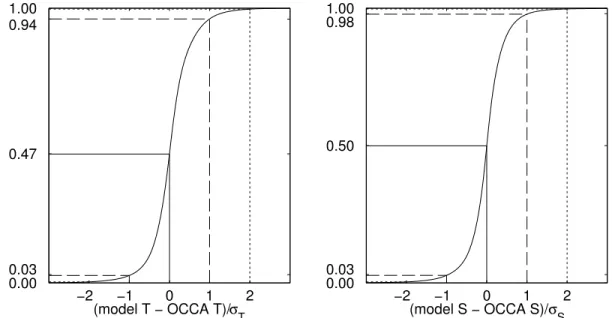
3-2 CDFs of normalized T/S misfits for Modern TS and OCCA . . . 105
3-3 CDFs of normalized atmospheric control variables for Modern TS . . . 107
3-4 CDFs of other normalized control variables for Modern TS . . . 107
3-5 Maps of Modern TS NSST and NSSS and misfits to OCCA . . . 108
3-6 Maps of Modern TS 300 m T/S and misfits to OCCA . . . 110
3-7 Maps of Modern TS 4000 m T/S and misfits to OCCA . . . 111
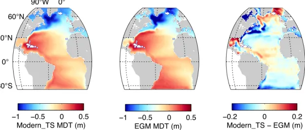
3-9 Mean dynamic topography in Modern TS and the EGM estimate . . . 115
3-10 MOC and 29◦N transport decomposition in Modern TS and OCCA . . . . 115
3-11 Meridional heat and freshwater transport in Modern TS . . . 116
3-12 Sea ice fraction maps in February and August in Modern TS . . . 118
3-13 Modern sea ice climatology (from Maurer 2007) . . . 118
3-14 Distribution of Schmidt et al. [1999]δ18 Owater observations . . . 121 3-15 Distribution of GEOSECSδ13 CDICobservations . . . 125 3-16 CDFs of normalizedδ18 Owater andδ 13 CDICmisfits for Modern Iso . . . 127
3-17 Modern Isoδ13 CDICmap at 2730 m with GEOSECS data overlaid . . . 128
3-18 Evaluation of asynchronous timestepping to accelerate optimization . . . . 132
3-19 Carry over controls as an effective means to extend state estimate length . . 134
3-20 Modern 80yrsδ13 CDICmap at 2730 m with GEOSECS data overlaid . . . . 136
3-21 CDFs of normalizedδ18 Owater andδ 13 CDICfor Modern 80yrs . . . 137
3-22 MOC and 29◦N transport decomposition in short and long state estimates . 139 3-23 Improvement in normalized NSST/NSSS misfits with optimization . . . 140
3-24 Improvement in normalized T/S misfits at 1100 m with optimization . . . . 141
4-1 Modern and ICE-5G LGM bathymetries . . . 147
4-2 CDF of the normalized misfit of NSSTs in LGM AllSSTs to MARGO. . . 154
4-3 Fit of first guess and LGM AllSSTs estimates to MARGO with explanation of wheel diagrams . . . 154
4-4 Fit of LGM NoForams and LGM AllSSTs to MARGO . . . 157
4-5 Fit of LGM Forams and LGM AllSSTs to MARGO . . . 157
4-6 Fit of LGM ForamsX2 and LGM Forams to MARGO . . . 159
4-7 Fit of LGM Upper and LGM AllSSTs to MARGO . . . 162
4-8 Misfit versus latitude for LGM Upper and WOA’09 to MARGO . . . 163
4-9 Maps of normalized misfits of LGM Upper to MARGO . . . 164
4-10 CDFs of normalized atmospheric control variables for LGM Upper . . . . 166
4-12 LGM Upper NSST maps and difference with WOA’09 . . . 168
4-13 Sea ice fraction in LGM Upper and difference from modern . . . 170
4-14 Comparison of LGM Upper sea ice presence to sea ice proxies . . . 171
4-15 Mean dynamic topography in LGM Upper and Modern TS . . . 172
4-16 AMOC and 29◦N transports in OCCA and LGM Upper . . . 174
4-17 Atmospheric adjustments in LGM Upper and comparison with modern . . 175
4-18 NSSTs in PMIP2 and LGM Upper LGM simulations . . . 177
4-19 Maps of misfit of PMIP2 NSSTs to MARGO foram assemblages . . . 178
4-20 Bar graphs of mean cost for LGM Upper and PMIP2 models . . . 180
4-21 Difference between Aug. and Feb. NSST in PMIP2 and LGM Upper . . . . 182
4-22 Maps of PMIP2 and LGM Upper winds . . . 183
4-23 Maps of LGM-modern differences for PMIP2 and LGM Upper winds . . . 184
4-24 Winter sea ice in PMIP2, LGM Upper, and proxy records . . . 187
4-25 Summer sea ice in PMIP2, LGM Upper, and proxy records . . . 188
5-1 Fit of LGM Upper and LGM Deep10yr against all proxies . . . 197
5-2 Fit of LGM Deep10yr and LGM Deep against all proxies . . . 197
5-3 Maps of NSSTs and anomalies in LGM Deep reveal model drifts . . . 198
5-4 AMOC and 29◦N transports in OCCA, LGM Deep10yr, and LGM Deep . . 201
5-5 Scatter plots ofδ13 Ccalcitemodel-data fit . . . 202
5-6 Maps of LGM Deepδ13 Ccalcite with MC08 records at 12 levels . . . 204
5-7 Scatter plots ofδ18 Ocalcite model-data fit . . . 205
5-8 Maps of LGM Deepδ18 Ocalcite with MC08 records at 12 levels . . . 207
List of Tables
2.1 Proxy records included in LGM state estimates . . . 39
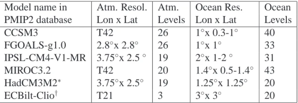
2.2 PMIP2 model configurations. . . 72
3.1 Model parameters used in all state estimates. . . 87
3.2 Modern atmospheric control uncertainties. . . 100
3.3 Full list of control variables used in the thesis. . . 122
3.4 AMOC transports in long-running state estimates, modern configuration. . . 137
Acronyms used in the thesis
With references where appropriate
AABW AntArctic Bottom Water
AMOC Atlantic Meridional Overturning Circulation
CCSM Community Climate System Model [Otto-Bliesner et al., 2006] CDF Cumulative Distribution Function
CLIMAP Climate: Long range Investigation, Mapping, and Prediction [CLIMAP
Project Members, 1976]
DIC Dissolved Inorganic Carbon DWBC Deep Western Boundary Current
ECCO Estimating the Circulation and Climate of the Ocean [Wunsch and
Heim-bach, 2007]
EOE Equilibrium Ocean Estimate
GEOSECS Geochemical Ocean Sections Study
GNAIW Glacial North Atlantic Intermediate Wwater H1/H2 Heinrich event 1/2
LGM Last Glacial Maximum
MARGO Multi-proxy Approach for the Reconstruction of the Glacial Ocean surface
[Waelbroeck et al., 2009]
MIT GCM Massachusetts Institute of Technology General Circulation Model [Adcroft
et al., 2004]
NADW North Atlantic Deep Wwater
PI Pre Industrial
PMIP Paleoclimate Modelling Intercomparison Project [Braconnot et al., 2007a] NCEP/NCAR National Centers for Environmental Prediction / National Center for
Atmospheric Research Reanalysis [Kalnay and coauthors, 1996] NSST Near Sea Surface Temperature
NSSS Near Sea Surface Salinity
SSS Sea Surface Salinity (directly at the surface)
SST Sea Surface Temperature (directly at the surface – the “skin” temperature) T/S Temperature and Salinity
Chapter 1
Introduction
The LGM is the period of maximum extent of terrestrial ice sheets during the most re-cent major glaciation in Earth’s history. Ice sheet extent appears to have been relatively stable over the period of 26.5 to 19 or 20 thousand years before present (26.5-19 or 20 kyr bp) [Clark et al., 2009], and sea level during this period was relatively stable at about 125 m below modern levels [Clark et al., 2009]. Atmospheric CO2 concentrations were also relatively stable at about 190 parts per million by volume (ppmv) during the LGM, as compared to about 280 ppmv during pre-industrial times [Schmitt et al., 2012].
Although some aspects of LGM climate are relatively well understood, the atmosphere and ocean circulation at the LGM remain particularly uncertain (see Chapter 2 for a thor-ough review). As there are relatively large numbers of proxy records available for the LGM Atlantic Ocean, there is a particularly good opportunity to better constrain conditions in this region. In this thesis, the state of the Last Glacial Maximum (LGM) Atlantic Ocean is re-constructed through a combination of proxy evidence and a dynamical understanding of ocean circulation. This work is guided by the following three lines of scientific inquiry.
1. Are there one or more Atlantic Ocean states that are consistent with known ocean dynamics and available LGM proxy records, given their uncertainties?
2. What magnitude of modern to LGM changes in oceanic and atmospheric state are required to obtain a consistent LGM Atlantic Ocean state? Are the required changes
uniform, or are regional patterns evident?
3. What Atlantic meridional overturning circulation state or states are consistent with available LGM deep ocean proxy data? More generally, what is required to constrain deep ocean water mass distributions and pathways with sparse deep ocean tracer data?
This chapter provides background and context for the rest of the thesis. Section 1.1 provides a more extended motivation for reconstructing LGM Atlantic Ocean conditions. Section 1.2 then describes limitations of common approaches to studying the LGM climate, and argues that synthesizing models and data through dynamical reconstruction is an im-portant, but infrequently used, approach. The dynamical reconstruction approach applied in this thesis is introduced, and previous applications of the technique are briefly reviewed to provide evidence for the suitability of the approach. The chapter concludes with a preview of the contents of the thesis.
1.1
The Last Glacial Maximum
Humankind is undertaking an unprecedented experiment by releasing massive amounts of CO2 and other greenhouse gases into the modern atmosphere – the anthropogenic climate experiment. While it is well accepted that serious shifts in climate are a potential, and even likely, outcome of this experiment, prediction of future climate change is a difficult exercise with many uncertainties [Solomon et al., 2007]. Climate models are the primary tool used to project anthropogenic climate change, but estimating how well such models simulate climates different from today’s is a challenge [Braconnot et al., 2012].
Fortunately, there is a source of data on how our planet responds under a variety of climate conditions: Earth’s geologic record includes clear evidence of past climates that were very different from today’s. Characteristics of past climates are inferred through proxy records – preserved chemical, isotopic, or physical characteristics that can be used to estimate past conditions. The mapping from preserved properties to past climate
charac-teristics relies on modern calibrations – demonstrations that modern climate characcharac-teristics are preserved in a consistent way in modern sediments.
A number of characteristics make the Last Glacial Maximum an excellent case study for dynamical reconstruction of a past climate.
• The LGM is a period of relative climate stability, apparently without large shifts in
land ice, sea level, or atmospheric CO2 concentrations [Clark et al., 2009, Schmitt et al., 2012]. This stability is key to interpretation of proxy records, and greatly simplifies application of climate models to the period (e.g. Braconnot et al. 2007a).
• Amongst relatively stable episodes of the last 100,000 years, the LGM is the most
drastically different climate from today’s. Given uncertainties in proxy records of climate, large changes are much easier to identify and quantify (e.g. Adkins et al. 2002).
• Atmospheric CO2 concentrations at the LGM were lower by about 90 ppmv than
at the pre-industrial [Schmitt et al., 2012], a difference that appears to have been important to sustaining colder LGM conditions [Shakun et al., 2012]. This period thus provides an important case study for the role of CO2 in climate [Schmittner et al., 2011]).
• Continental configurations were very similar to today’s [Peltier, 2004], simplifying
attribution of climate changes.
• The LGM is one of the most extensively studied periods in Earth’s history, so that
relatively large numbers of proxy records are available. Uncertainties in proxies themselves, and in the dating of the proxy records, are generally lower for the LGM than for periods further back in time.
• Substantial effort has been made to build large, quality-controlled compilations of
proxy records (e.g. CLIMAP Project Members 1976, Marchitto and Broecker 2006, Waelbroeck et al. 2009, Marchal and Curry 2008). These compilations greatly sim-plifying the task of using proxy records.
It is now apparent why the LGM is appropriate for dynamical reconstruction, and why the results are important to current climate concerns. It is, at this point, less obvious why it is sensible to focus on the LGM Atlantic Ocean state. The Atlantic Ocean is one of the best studied regions for the LGM (see Chapter 2), and is also a relatively well-understood part of the modern climate (see Chapter 3). The Atlantic is also dynamically important as a deep water mass formation region. Finally, significant shifts in Atlantic Ocean state have been proposed to have occurred between the LGM and today (e.g. Lynch-Stieglitz et al. 1999b, Curry and Oppo 2005), providing a number of intriguing hypotheses to test.
1.2
Dynamical reconstruction
Most studies of LGM ocean circulation focus on (1) proxy records, which are often inter-preted with the aid of qualitative ideas about shifts in ocean circulation; or (2) dynamical models of LGM changes (e.g. theories, idealized models, coupled climate models), which are sometimes compared in a qualitative sense with selected proxy records. These ap-proaches have contributed much to our understanding of LGM climate (Chapter 2 presents a full review), but there are risks in focusing too heavily on one approach. The qualitative ideas of ocean circulation sometimes used to interpret proxy records may be physically unrealistic, and the state obtained in dynamical models can be quite far from observations, making it difficult to apply inferences made from the models.
The need to move from qualitative to quantitative model-data comparisons has recently become a focus for both the LGM modeling community [Braconnot et al., 2012] and the LGM proxy community1. There is also increasing recognition from the broader modeling community of the potential of paleo model/data comparisons to improve model forecasts of future climate [Schmidt, 2010].
Dynamical reconstruction moves beyond quantitative comparison to build estimates of 1The Comparing Ocean Models with Paleo-Archives (COMPARE) workshop, held in March 2012 in
Bremen, Germany, focused on the topic of model/data comparisons and approaches to synthesizing models and data.
climate that are consistent with both model and data. The exercise of building a model-data synthesis brings to the investigator a number of advantages. First, serious consideration can be given to the uncertainties and biases of both models and data, providing a more holistic view of the problem at hand. Second, a quantitative measure for “success” is defined a priori, with explicit weighting of the relative importance of diverse data constraints. This approach permits formal statistical hypothesis testing.
Quantitative model-data synthesis has been previously applied to the LGM Atlantic (see Section 2.4.2 for a thorough review). For this thesis, the ocean state is estimated us-ing the method of Lagrange multipliers, whereby a least squares fit of a dynamical model to the proxy data is computed using an algorithm based on the model adjoint [Wunsch and Heimbach, 2007]. In this approach, the model-data misfit is reduced by computing improvements to uncertain initial and boundary conditions (the control variables). Quanti-tative uncertainties assigned to all proxy records and to the control variables play as much a part in the solution obtained as do the data themselves. Section 3.2 provides a more com-plete overview of the state estimation methodology used in the thesis. For now we simply note that, as compared to previous model-data syntheses for the LGM Atlantic, this thesis uses a more complete dynamical model and a larger number and greater diversity of proxy records.
The tool applied in this thesis to build dynamical reconstructions is the Massachusetts Institute of Technology General Circulation Model (MIT GCM) [Marshall et al., 1997, Ad-croft et al., 2004] and its adjoint [Heimbach et al., 2005]. Estimates of ocean circulation and properties developed using this tool in combination with data are called ocean state
estimates and the process of making the model-data synthesis is called ocean state estima-tion. The MIT GCM and its adjoint have been applied to develop a variety of modern ocean
state estimates. A particularly substantial modern effort is the Estimating the Circulation and Climate of the Ocean (ECCO) project, a large, multi-institution project that has fo-cused primarily on estimating the global ocean circulation [Stammer et al., 2002, Wunsch and Heimbach, 2007, 2012, in press]; vast numbers of observations have been successfully
incorporated in these state estimates, including, for example, hydrography, satellite obser-vations of sea surface temperature and sea surface height, autonomous float data, and data from bottom pressure recorders. Examples of regional ocean state estimates include the Eastern Atlantic Ocean [Gebbie et al., 2006], the Southern Ocean [Mazloff et al., 2010], and the Labrador Sea [Fenty, 2010, Fenty and Heimbach, 2012]. These estimates have incorporated a wide diversity of observational data, and each estimate has proven useful in understanding new aspects of the modern ocean circulation.
Due to the poor dating resolution of sediment cores from the LGM period, and the spar-sity of LGM proxy observations, LGM proxy records are typically assumed to represent average conditions over thousands of years; for some proxies, it is possible to estimate con-ditions in specific seasons (e.g. summer or winter), but these estimates still represent a very long term mean of summer or winter conditions over the LGM period. Due to these limita-tions in the timescales that can be reconstructed with available data, a seasonal steady state assumption is adopted here – that the LGM Atlantic can be adequately represented with a seasonally varying, but otherwise stable in time, steady state (a seasonal steady state). Previous LGM model-data syntheses have generally made a direct steady state assump-tion (no seasonal cycle), and have built this assumpassump-tion into the model framework (see Section 2.4.2).
Here, instead of building a steady state assumption into the model, an alternate ap-proach is taken: to search for an ocean state estimate that satisfies the seasonal steady state assumption. A new type of ocean state estimate is defined: an equilibrium ocean estimate (EOE) is an estimate of ocean state that is
1. consistent with known dynamics,
2. consistent with available data given their uncertainties, and
3. consistent with a steady state assumption (whether fully steady or cyclic in nature). It is likely that there are a number of different approaches that could be used to achieve these three goals. In this thesis, the philosophy used by the paleo climate modeling com-munity is adopted (see Section 2.3.1): that a long-running model simulation with limited
drift is indicative of a quasi-steady (or quasi-equilibrium) circulation. Long-running model simulations have another advantage: interior ocean properties are set largely by the at-mospheric forcing applied to the model, rather than the initial properties from which the model was started. For a problem such as reconstructing the LGM ocean state, a full dy-namical connection between atmospheric forcing and interior ocean conditions. Without such a connection, one can not investigate, for example, what deep interior ocean data imply about surface boundary conditions.question that has arisen
1.3
Terminology
In drawing upon proxy evidence of past climates, modern observations, forward models, and inverse modeling techniques, this thesis necessarily relies on much terminology, the exact meaning of which may sometimes be unclear. To aid the reader, a list of acronyms used in the thesis is provided on page 19 and the following paragraphs describe how key terminology is used in the thesis.
The Last Glacial Maximum. Exact definitions of the LGM time period vary. The
estimates of LGM state developed in this thesis rely on proxy record compilations that either define the LGM to span 19-23,000 years ago [Waelbroeck et al., 2009] or 18-21,000 years ago [Marchal and Curry, 2008]. The first definition is followed here - that the period under study spans 19-23,000 calendar years before present (19-23 kyr bp).
Proxy record. In paleoclimate literature, the word “record” often refers to
measure-ments made on a sequence of samples from, for example, a sediment or ice core; in the standard terminology, a proxy record is a time-varying sequence of data corresponding to a particular section of sediment or ice core material. In this thesis, only the LGM time period is discussed, and all compilations of proxy evidence used in the thesis have (1) assumed the LGM spans a given range of years, (2) computed an average of available sediment core evidence over that period, and (3) have reported only the average conditions over the LGM period. Therefore, for the purposes of this thesis, a proxy record (or simply record) is a
single estimate of LGM conditions at a given geographic location.
Near sea surface temperature. Sea surface temperature (SST) can mean different
things to different communities. Those who estimate SST from satellites are truly mea-suring the skin temperature at the surface of the ocean. In conditions of strong thermal stratification (i.e. in summer), the skin temperature may apply over only the top few mil-limeters. Likewise, meteorologists and atmospheric dynamicists may be interested in SST only as a boundary condition on atmospheric dynamics; this boundary condition is the skin temperature of the surface ocean. The term SST is avoided in this thesis and near sea sur-face temperature (NSST) is used instead to remind the reader that we are not discussing the skin temperature. In the work presented herein on modern conditions (Chapter 3), NSST is taken to be the temperature of the upper most cell of the model, which is 10 m thick. In the work presented on LGM conditions (Chapters 4 and 5), NSST is taken to be the mean tem-perature of the top three cells of the model, a depth of 30 m in total. NSST reconstructions for the LGM are based on organisms that inhabit a variety of depths in the water column; 30 m is taken as a conservative estimate of the potential habitats of these organisms.
1.4
Structure of the thesis
In this thesis, I argue that LGM ocean conditions can be best understood through dynamical reconstruction. It could be argued that the circulation estimates presented in this thesis are the most complete dynamical reconstructions of the LGM Atlantic Ocean currently avail-able. The thesis presents a number of contributions to understanding of the LGM Atlantic that would not have been possible without a dynamical reconstruction. Despite the power of dynamical reconstruction, incorporating data and models in a single estimate or recon-struction is a challenge: it requires honest consideration of the limitations and potential biases of both models and data (which are often poorly known), and the technical machin-ery involved is difficult to learn and computationally expensive to apply. The contributions and remaining challenges of this work are described in the remainder of the thesis, which
is structured as follows.
Chapter 2 surveys current knowledge of the LGM Atlantic, with detailed discussions of proxy evidence, numerical modeling studies, and previous approaches to dynamical recon-struction. A particular contribution of this chapter is an evaluation of the relative ease with which available proxy types could be incorporated in a model-data synthesis.
In Chapter 3, a framework for ocean state estimation that is appropriate to study of paleo circulation is presented. The utility of this framework is explored in the context of the mod-ern ocean circulation – a system that is much better observed and understood than the LGM ocean. An approach to modelingδ13
CDICandδ
18
Owater is presented and tested in state
es-timates constrained by modern water column measurements ofδ13
CDICandδ
18
Owater. Two
techniques for extending the length of ocean state estimates, asynchronous timestepping and carry-over control, are described and shown to be appropriate and effective. Signifi-cant limitations of the state estimation framework are identified.
Estimation of the LGM upper ocean state is the focus of Chapter 4. Four diverse near sea surface temperature (NSST) proxy compilations are used to constrain the estimates. The chapter explores disagreement amongst the datasets, the extent to which the LGM NSST data require an atmospheric state significantly different from today’s, and the con-sistency of the state estimates with withheld data. Results are compared to existing coupled model simulations of the LGM climate.
Chapter 5 is more exploratory in nature. State estimates are presented that are con-strained by deep ocean proxy records (benthicδ13
Ccalcite andδ
18
Ocalcitedata, see Chapter 2
for details on these proxies) in addition to the NSST data used in Chapter 4. The con-sistency of these data with a meridional overturning circulation different from today’s is explored.
Finally, Chapter 6 concludes the thesis. A vision for the future of ocean state estimation is presented, along with a discussion of what is required to enable state estimation for scenarios in which a steady state assumption is required. Novel contributions of the thesis are summarized, as are limitations. Promising directions for future progress are presented.
Chapter 2
Last Glacial Maximum Atlantic
This chapter summarizes what is currently known or hypothesized about the state of the Last Glacial Maximum (LGM) climate, and particularly about the state of the LGM At-lantic Ocean. Due to the breadth and depth of previous work focused on the LGM, this review cannot be comprehensive. Instead, the focus is on previous work that is particularly important as background for the rest of thesis. The chapter begins with an overview of the LGM climate in Section 2.1. Section 2.2 describes proxies for upper ocean and deep ocean state at the LGM, and includes a detailed discussion of potential sources of uncertainty and bias in reconstructions of climate with these proxies. Section 2.3 summarizes results obtained with traditional forward models of the LGM. Efforts to seriously consider models and data together are described in Section 2.4, which covers previous work in quantitative model-data comparison as well as in model-data synthesis. Section 2.5 describes which datasets were chosen as data constraints in the thesis and why, and Section 2.6 concludes the chapter.
In reading this chapter (and indeed the whole thesis), it is important to keep in mind that observations or modeling results from a specific geographic region cannot be used to make global inferences. Indeed, the global climate system is connected on a multitude of spatial and temporal scales, so that changes in climate in one region may be associated with changes of an opposing sign in another region (e.g., shifts in the westerlies would
cause increased wind speed in some regions and decreased wind speed in others). Even climate characteristics for which the modern-LGM changes could be predominantly of one sign (e.g., LGM air temperatures were generally colder than today’s), the magnitude of change can have strong regional dependencies.
2.1
Geography and atmospheric State
Physical geography. The location of the land masses at the LGM was very similar to that
of today, though large terrestrial ice sheets and the associated sea level lowering caused sub-stantial changes in Earth’s geography. The timing of the LGM sea level lowstand appears to be in good agreement with the timing of the maximum extent of ice sheets and mountain glaciers; the peak LGM glaciation occurred from 26.5 to 19 ka, and global ice volume (and therefore sea level) was relatively stable during this period [Clark et al., 2009]. Long term sea level records from Barbados [Fairbanks, 1989], the Sunda Shelf of Indonesia [Hanebuth et al., 2000], and the J. Bonaparte Gulf region of northern Australia [Yokoyama et al., 2000] are consistent with a globally averaged sea level change from today to the LGM of about 125 m. Interpretation of local sea level changes are complicated by isostatic adjustment -the dynamic adjustment of -the as-thenosphere to accommodate -the mass of -the lithosphere. Ice sheet models that include the effect of isostatic adjustment can be used to infer global sea level changes from relative sea level records; this approach was used by Peltier [2004] to estimate an LGM sea level lowering of 125 m and by Clark et al. [2009] to estimate a lowering of 130 m.
Due to lowered sea levels, several key changes in ocean bathymetry occurred that af-fected the Atlantic Ocean: the Bering Strait was closed, shallow continental shelves (such as that off the east coast of North America) were exposed, Hudson Bay was exposed, and all sills were shallower by about 125 m (see Figure 2-1). The storage of freshwater in ter-restrial ice sheets also resulted in an increase in mean ocean salinity of about 1.1 relative to today [Adkins and Schrag, 2001]. Due to the nonlinear dependence of density on
tempera-Figure 2-1: Overview of LGM ice sheets (solid white regions), coastlines (overlaid in black on modern map in gray), and terrestrial temperature anomalies in◦C from pollen and macrofossil data (colored circles, size indicates significance). Ice sheets and coastlines are a blended combination of three recent ice sheet reconstructions. Cropped version of figure from Braconnot et al. [2012]; see references therein for data sources.
Figure 2-2: Comparison of ICE-4G and ICE-5G elevation across the Laurentide ice sheet at 55◦N (left). On the right, ice sheet extent as reconstructed by ICE-5G is outlined in white, and the 55◦N section is marked in black. Figure from Li and Battisti [2008].
ture and salinity, the increase in mean salinity at the LGM implies that salinity likely played a more significant role in controlling the LGM density field than it does today [Adkins and Schrag, 2001].
LGM global mean sea level is relatively well-constrained and permits direct estimation of LGM global glacial ice volume. Ice sheet topography is much more difficult to estimate, but is important to constrain as it impacts many aspects of atmospheric state including the wind field. The Environmental Processes of the Ice Age: Land, Oceans, Glaciers (EPI-LOG) project was an effort to reconstruct the state of the Earth in glacial states; a special issue collection of EPILOG papers [Clark and Mix, 2002] focused on records of ice sheet extent, sea level change records, models of ice sheets and glacial isostatic adjustment, and geochemical ice volume proxies. Siegert [2001] provides an extensive overview of obser-vations and models of ice sheets in the Late Quaternary. Siegert [2001] notes that, although physical indicators such as glacial moraines and glacial scour provide a relatively accurate picture of ice sheet extent, ice sheet thickness is much more difficult to estimate from sur-ficial geologic evidence. Relative sea level records collected worldwide have been used in concert with an ice sheet model and a model of isostatic adjustment to infer the mass of individual LGM ice sheets [Peltier, 2004]. The Peltier [2004] ICE-5G gridded estimate of LGM ice sheet topography, coastlines, and ocean bathymetry has proven useful to LGM modeling efforts (e.g., Braconnot et al. 2007a). In using these estimates it must be remem-bered that LGM ice sheet topography remains uncertain (see Figure 2-2).
The majority of available dust records show glacial periods to have been generally dustier and interglacials to have been more vegetated [Rea, 1994, Yung et al., 1996, Hesse and McTainsh, 1999]. Greenland and Antarctic ice core records show a 2 to 20 fold in-crease in dust deposition rates at the LGM as compared with the present while low and mid-latitude marine sediment core records show up to a 5 fold increase [Kohfeld and Har-rison, 2001]. In the Kohfeld and Harrison [2001] compilation of data from ice cores and marine sediment cores, nearly all sites show increases in dust deposition at the LGM com-pared to today. It is commonly thought that increased dust fluxes at the LGM are at least
partially caused by drier terrestrial conditions with significant changes in vegetation, at least in some regions [Hesse and McTainsh, 1999, Kohfeld and Harrison, 2001]. The Andean region is an exception: records indicate that the region is actually drier during interglacials than during glacials [Rea, 1994]. A global compilation of lake level reconstructions (see supplementary material of Braconnot et al. 2012 indicates that LGM conditions may have been drier than today in the tropics, but wetter than today in the low-mid latitudes, a sce-nario supported by the PMIP2 models [Boos, 2012].
Atmospheric state. Reconstructing the atmospheric state at the LGM with proxy
ob-servations is a major challenge. Mahowald et al. [1999] compare a model of the dust cycle at the LGM with proxy records and find evidence for a reduced hydrologic cycle at the LGM. As shown in Figure 2-1, pollen and macrofossil based proxies indicate LGM tem-peratures over land were typically 5-10◦C colder than modern with even larger changes in the Southeastern United States. The intense LGM cooling in this region and the relatively warm conditions in Alaska are both consistent with the generally accepted notion that the Laurentide ice sheet caused a substantial shift in atmospheric circulation (see below).
It is sometimes assumed that high atmospheric dust concentrations (and therefore high depositional fluxes) indicate high wind speed. In fact, this assumption is not supported by observations [Rea, 1994] nor by the physics of sediment transport. Instead, in the modern climate, high atmospheric dust concentrations have been linked to low rainfall in source regions [N’Tchayi et al., 1994, Ekstrom et al., 2004]. Dust flux rates can also be linked to rainfall rates in the deposition area since dust deposition is higher during rainfall [Kohfeld and Harrison, 2001].
While dust concentrations cannot be used as a proxy for wind speed, grain size distri-butions have been used for this purpose [Rea, 1994, Parkin and Padgham, 1975]. Clemens [1998] did a careful study of modern eolian deposition in the Arabian Sea to compare char-acteristics of the dust with measured charchar-acteristics of the wind field; eleven sediment traps were used over a full annual cycle and compared against meteorological data on wind speed
and barometric pressure. A high correlation of eolian grain size with barometric pressure (r = -0.91), and with wind speed (r = 0.84) was found. Other researchers have linked the quantity of magnetite in aeolian dust to transport processes such as wind speed [Maier and Scholger, 2004] based on the wind power required to deflate heavier magnetite particles from source regions and transport them. Magnetite quantity is a convenient measure for application to paleo-environments as magnetic susceptibility is relatively straightforward to measure. Some information about wind direction can be inferred by matching character-istics of deposited dust with charactercharacter-istics of source regions. This approach of identifying dust “fingerprints” requires that the measured dust properties be part of the dust or be transported with the dust, be distinctive of the source region, and be conservative during transport [Grousset and Biscaye, 2005]. Biological tracers such as opal phytoliths, fresh-water diatoms, and pollen can also be used to constrain the latitude of a dust source region. The most promising tracers for better constraining dust sources appear to be radiogenic isotopes such as strontium, neodymium, and lead [Grousset and Biscaye, 2005]
In a survey of many available proxy records of the dust cycle, Kohfeld and Harrison [2001] conclude that dust records from Greenland and Antarctic ice cores do not indi-cate significant changes in the LGM high latitude atmospheric circulation relative to today; Hesse and McTainsh [1999] agree, finding that increased dust fluxes to Antarctica at the LGM are due to increased source region aridity at the LGM, rather than to windier condi-tions. In contrast, LGM proxy records are used by Yung et al. [1996] to infer an increased wind field in both hemispheres and by Delmonte et al. [2004] to infer a southward shift of the southern hemisphere polar vortex between 20 to 10 kya. Parkin and Padgham [1975] infer changes in the trade winds at the LGM based on observed changes in grain size. Florineth and Schluchter [2000] combine geologic mapping of European alpine glacier lo-cations through time with other terrestrial records such as lake levels; they infer that the po-lar front may have been centered near 44◦N at the LGM, leading to a southerly atmospheric circulation (the modern circulation is predominantly westerly) and lower precipitation in central and northern Europe at the LGM relative to today.
Given the relative paucity of proxy records of atmospheric state, climate models have been heavily applied to estimate LGM conditions. Coupled models of the LGM climate will be discussed in Section 2.3.1; in this section we note a few model results that are specific to understanding LGM atmospheric conditions. The effect of the large terrestrial ice sheets on atmospheric stationary waves is relatively well understood [Cook and Held, 1992, Jackson, 2000, Roe and Lindzen, 2001]; with regard to the Laurentide ice sheet, the Jet Stream was likely shifted northward to the west of the ice sheet (thus explaining the warm Alaskan temperatures seen in Figure 2-1) and was pushed south to flow around the southern boundary of the ice sheet over the continental United States (thus explaining cold LGM temperatures in the Southeastern United States in Figure 2-1). Li and Battisti [2008] investigate atmospheric dynamics in a single coupled model simulation of the LGM (the Community Climate System Model, version 3 – CCSM3) and find stronger, more zonally oriented atmospheric jets over the Atlantic Ocean as compared to today. Li and Battisti [2008] also find that transient eddy activity is weaker over the Atlantic Ocean in the LGM simulation than in the modern one, implying reduced storminess at the LGM.
Rojas et al. [2009] analyze a variety of coupled model simulations of the LGM to in-vestigate changes in the Westerlies in the Southern Ocean. These authors find that while surface equator to pole temperature gradients were larger in the LGM models than in the modern climate, the tropospheric temperature gradients are actually reduced for the LGM simulations; decreased winds near the surface and in the upper troposphere result [Rojas et al., 2009]. Toggweiler et al. [2006] propose that significant shifts occurred in the latitudi-nal position of the westerlies in the Southern Hemisphere between the LGM and today and that these shifts played a major role in deep ocean circulation differences between the LGM and today. They review a few proxy-based studies indicating that the Southern Hemisphere westerlies could have been as much as 7-10◦further north at the LGM than today; they also review observational evidence that the modern westerlies are slowly shifting poleward as a result of global warming.
2.2
Proxies of LGM ocean state
The LGM is a heavily studied period in the geologic record, and many proxies that cannot be used for older periods work well for the LGM (e.g., radiocarbon). A major challenge in designing a dynamical reconstruction of LGM ocean state is to decide which proxy types, and which specific proxy records, are most appropriate for inclusion in a model-data synthesis. This section describes a variety of proxies of LGM ocean state. For each proxy type, an evaluation is made of how appropriate the data are for quantitative model-data comparisons or syntheses with that proxy type. Note that the fundamental issues are essentially the same for either model-data comparisons or syntheses, and the evaluations herein are meant to apply to either. Note that, although not considered in the evaluations of this chapter, many more practical issues arise in practice in building a model-data synthesis than in quantitative model-data comparisons.
The following conditions are key to meaningful model-data comparisons or synthe-ses: a mapping exists between properties recorded by the proxy and properties that can be incorporated in existing ocean models, quantitative uncertainty assignments can be made for the data, sufficient numbers and distribution of records exists to warrant a comparison or synthesis effort, and the data must be publicly available or otherwise accessible to the investigator. These evaluations represent a personal scientific judgement, and others will certainly disagree with some aspects of the evaluations. Nonetheless, it is hoped that these evaluations will aid other investigators who are interested in quantitative analysis of models and data together.
This section is organized as follows. Section 2.2.1 provides a general discussion of po-tential uncertainties and biases in marine proxies; uncertainties play in model-data synthe-sis, and thus must be carefully considered. Sections 2.2.2 and 2.2.3 then describe selected proxies for upper and deep ocean conditions, respectively. As a preview of what is to come in the rest of the thesis, Table 2.1 lists the proxies used in later chapters of the thesis to constrain our estimates of LGM ocean state; these proxies are more thoroughly reviewed here than proxies that have not been included in the state estimates.
Source Parameter # records Reference
Foraminiferal assemblage SST 174 Kucera et al. [2005b] Dinoflagellate cyst assemblage SST 52 De Vernal et al. [2005]
Alkenones SST 54 Rosell-Mel´e et al. [2004]
Mg/Ca SST 33 Barker et al. [2005]
Benthic foraminifera δ18
Ocalcite 169 Marchal and Curry [2008] Benthic foraminifera δ13
Ccalcite 147 Marchal and Curry [2008]
Table 2.1: Summary of proxies included in LGM state estimates presented in the thesis. The number of records that fall in the model domain is noted for each proxy type. The first four/last two proxies are used to infer upper/deep ocean conditions. A total of 629 proxy records are incorporated in the LGM state estimates.
2.2.1
Introduction to potential uncertainties and biases
As will be clear in Sections 2.2.2 and 2.2.3, each marine proxy is affected by a distinct combination of uncertainties and biases, so that each has unique advantages and disadvan-tages. This section provides an overview of potential pitfalls affecting interpretation of marine proxies. The section begins with a list of general issues, a summary that will then be made more concrete with a case study of uncertainties and biases forδ18
O as a proxy. Instrumental precision in the measurement of the proxy itself is often quite small and can be misleading if quoted in isolation. Care must be taken to incorporate other, often larger, uncertainties associated with proxy interpretation. Some of these are as follows.
• Inter-laboratory differences in instrument calibration or in preparation techniques
can lead to biases between samples prepared in different laboratories (see, e.g., Os-termann and Curry 2000).
• Although proxies are typically assumed to represent either seasonal, annual, or
long-term mean climate properties, proxies may carry a strong signal of more occasional but strong events. Examples include spring bloom events in the high-latitudes that can affect inferences of annual mean temperature from planktonic proxies (see, e.g., Dale 2001), and submarine landslides that complicate interpretation of grain size records (see, e.g., McCave and Hall 2006).
• Proxies are typically converted into a single climate variable through techniques such
as correlation of modern measurements with modern climate properties. In reality, most proxies correspond to multiple environmental variables (see, e.g., Morey et al. 2005). The assumption that a single climate characteristic dominates the proxy’s variation back in time leads to uncertainties that are difficult to quantify.
• Several issues are largely specific to planktonic proxies. First, what plankton record
in their own habitat may not match what is preserved in a sediment core; for exam-ple, biases can occur due to the impact of dissolution (see, e.g., Barker et al. 2005) or diagenetic alteration (chemical changes that occur within the sediment after deposi-tion on the seafloor). Second, the representativeness of a given organism to a specific depth range of the water column may be poorly constrained (see, e.g., Farmer et al. 2007).
• For proxies that record conditions at the seafloor, there is a mismatch between what
is recorded by the proxy and what can be adequately represented in today’s climate models. Benthic organisms live on or in the sediment, an area that is in a boundary layer with a very different dynamical regime than the rest of the water column. With current computational capabilities, climate models are run at resolutions far too low to accurately capture boundary layer physics. Just as an example, it is not uncommon to have vertical jumps of 500 m in elevation between adjacent grid cells in deep layers of ocean models (see, e.g., Forget 2010).
To make the discussion of potential uncertainties more concrete, uncertainties associ-ated withδ18
Ocalcite as a proxy are now used as a case study. This proxy is chosen because
there are particularly extensive uncertainty analyses available in the literature. A particu-larly valuable resource is a thorough review in Waelbroeck et al. [2005] of uncertainties in measurements ofδ18
Ocalcite in planktonic foraminifera from Holocene sediment samples.
Unless otherwise noted, the following discussion is based on Waelbroeck et al. [2005]. Although standard deviations of 0.05-0.06h can be obtained in repeated measurements of a single sample ofδ18
can be introduced with small sample sizes or when the sample’s isotopic composition is far from that of the reference standard. A correction of this last bias has been developed [Oster-mann and Curry, 2000] and is applied to new measurements in most laboratories; unfortu-nately, it is sometimes unclear whether the correction has been applied to a given published record, particularly for old measurements. In addition, differences in cleaning and sam-ple preparation techniques can introduce an uncertainty on the order of 0.2h. Measured
δ18
O values have sometimes been found to depend on fossil foraminifera size, and this dependency can vary across species, size fractions, and regions.
Measurements of the δ18
O on individual foraminifera of a given species in a specific depth or time interval will show a range of δ18
O values. This intraspecies variability is due to the recording of seasonal and short-term water column variability (most shallow-dwelling planktonic foraminifera have a 2-4 week lifecycle, Schiebel and Hemleben 2005); the influence of bioturbation and the co-occurrence of several genotypes of a morphos-pecies can also introduce variability. For a single interval near sediment core tops, theδ18
O range observed amongst individual shells is ≈ 1.2 − 1.5h for planktonic species such
as Orbulina universa, Globigerinoides sacculifer, and pink and white G. Ruber and can exceed2h for thermocline dwelling species such as Neogloboquadrina dutertrei and Pul-leniatina obliquiloculata. For a subset of data and assumed instrument precision of 0.06h,
Waelbroeck et al. [2005] estimate that use of 20 shells implies a precision of 0.09-0.19h for planktonic foraminifera. Due to much lower variability in water properties at depth, precision for benthic species is significantly better. Post-depositional processes can also alter the observedδ18
Ocalcitesignal: bioturbation may act to dampen the Holocene to LGM
signal, and partial post-depositional dissolution may alter theδ18
Ocalciteof the foraminifera.
Uncertainties associated with these processes are not well-constrained. Records of δ18
Ocalcite tend to over-represent conditions during peak growing seasons
and peak years, an issue that varies amongst genera. As an example, Mulitza et al. [2003] find that for a station off Mauritania at Cape Blanc, G. ruber and G. sacculifer seem to record summertime SSTs, O. universa seems to record annual mean conditions, and G.
bulloides and G. inflata record conditions more similar to winter conditions. Another issue
of concern is that many genera can be found in a wide range of depths, calling into question their use as proxies for sea surface conditions. However, Mulitza et al. [2003] show that at an eastern equatorial Atlantic station, measuredδ18
Ocalciteis in line with expected values
very near the surface, implying that although they observed foraminifera living at a wide range of depths, the calcification depth for the foraminifera genera they studied was likely in the surface mixed layer.
Although proxies are typically used to reconstruct a primary environmental variable, they are often impacted by multiple climate conditions. For example, a unit change in pH has an approximately 1h effect on δ18
Ocalcite [Zeebe, 1999]; if surface ocean pH was
significantly higher at the LGM than today, as claimed by Sanyal et al. [1995], this effect could introduce a significant biases.
Quantifying all potential uncertainties and biases and using them to compute an overall uncertainty is a formidable challenge. Existing compilations with overall uncertainty esti-mates include the Waelbroeck et al. [2005] compilation of 2100 measurements of Holocene planktonic foraminifera δ18
Ocalcite and the Marchal and Curry [2008] compilation of 198
Holocene and 180 LGM measurements ofδ18
Ocalciteon benthic foraminifera. Each of these
studies assigned a uniform uncertainty of 0.2h to allδ18
Ocalcite records.
2.2.2
Upper ocean state
The surface ocean is the connection between the atmosphere and the rest of the ocean: it serves as a key boundary condition on atmospheric dynamics, and is the region where nearly all deep ocean properties originate. The portion of the upper ocean that receives solar insolation, the euphotic zone, is also the most productive zone in the ocean. Fortunately, characteristics of the upper ocean from the past are relatively well-preserved in sediment cores. A number of proxy approaches are described here: four different plankton-based proxies to reconstruct temperatures near the sea surface (near sea surface temperature or NSST), two plankton-based proxies to reconstruct sea ice distributions, and multi-proxy
approaches.
Near sea surface temperatures1. The most extensive compilations of LGM NSST
proxies are those of the CLIMAP [CLIMAP Project Members, 1976], GLAMAP [Sarn-thein et al., 2003], and MARGO [Kucera et al., 2005a] projects. Two factors accounts for this focused attention on reconstructing LGM NSSTs: (1) as compared to other environ-mental variables, NSST is relatively straightforward to reconstruct from proxy evidence, and (2) as a key boundary condition for the atmosphere, NSST is an important parameter for realistic model simulations of LGM atmospheric conditions. The MARGO project, the most recent NSST compilation effort, developed comprehensive, global compilations based on a variety of proxy types. The project focused on making data accessible to modelers, and substantial effort was dedicated to providing quantitative uncertainties on each proxy record [Waelbroeck et al., 2009].
Due to their high quality and comprehensive nature, in the context of NSST recon-struction, only the MARGO compilations are considered here. The four MARGO com-pilations that provide some coverage in the Atlantic Ocean are described in this section: foraminiferal assemblages, dinocyst assemblages, Mg/Ca, and alkenones. The following applies to all four compilations. A relatively narrow definition of the LGM, from 23-19 cal ka, is used; this corresponds to the period of maximum continental ice extent [Kucera et al., 2005a]. To simplify comparisons, all modern calibrations used in MARGO were made using the 1998 World Ocean Atlas. Uncertainty estimates were assigned to all data; these incorporate uncertainties associated with dating, calibration, and with the number of samples available in the 23-19 kyr bp time slice. The specific details of MARGO uncer-tainty estimates are provided in Appendix A. Note that the evaluation of NSST proxies for model-data synthesis is postponed until all of the NSST proxies have been described.
NSSTs from assemblages of planktonic foraminifera. Planktonic foraminifera, or
forams, are zooplankton that are found throughout the modern and Last Glacial Maximum 1NSST is used throughout this thesis in place of SST to avoid confusion with the usage of SST in
mete-orology as a term for the ocean’s surface skin temperature. Note that in the paleoceanographic literature the term SST, and not NSST, is used.
oceans. Although foraminifera make up a small fraction of all zooplankton, their CaCO3 shells constitute a major component of ocean sediments [Schiebel and Hemleben, 2005]. Assemblage or transfer-function based approaches are used to reconstruct near sea sur-face temperatures (or other climate parameters) based on the calcium carbonate (CaCO3) shells of foraminifera recovered from sediment cores. The assumption used in assem-blage and transfer function based approaches is that the number and type of planktonic species preserved in a sediment core can be used to infer climate conditions in the past. These techniques proceed as follows: (1) catalog the species assemblages of a variety of modern habitats for which instrumental records are available, (2) analyze the species assemblages of sediment samples from past climates, (3) identify similarities between the past climate assemblages and observed modern assemblages using multiple regression, and (4) use the regression to infer past climate conditions. Reconstruction of LGM NSSTs with foraminiferal assemblages has a long history (e.g. CLIMAP Project Members [1976], Pflaumann et al. [2003], Kucera et al. [2005b]). The MARGO compilation [Kucera et al., 2005b, Hayes et al., 2005] uses five geographically constrained calibration data sets, in-cluding three in the Atlantic: the South Atlantic (N = 321 modern observations), North Atlantic (N = 862), and Mediterranean Sea (N = 145). This approach reduces noise and false associations between distinct populations.
Figure 2-3 (top row) shows maps of the difference between WOA’09 and MARGO foram assemblage based annual, winter, and summer mean LGM near sea surface temper-atures; the same data are plotted against latitude in Figure 2-4 (top row). There are 174 foram assemblage based NSST records in the Atlantic domain considered in this thesis (in this thesis, “record” is used to refer to individual proxy data points, not to a time-series of data). Figure 2-3 (top row) reveals notable gaps in data coverage in the Gulf Stream, mid-latitude gyre, and Labrador Seas, and the data locations are biased towards continental margins. The WOA09 - MARGO anomalies show high spatial coherence, implying high spatial coherence in the MARGO foram assemblage based NSST reconstructions. Strong LGM cooling is evident in the subpolar gyre, especially south of Iceland; in the eastern half
of the low-latitude oceans; and in the Norwegian Sea (northeast of Iceland) (Figure 2-3). Inferred temperature changes are small in the western half of the basin and in the Greenland Sea (northwest of Iceland). Annual, winter, and summer anomaly patterns are similar with one exception: the western equatorial region shows a stronger LGM cooling in the summer than in the winter. As is especially apparent in Figure 2-4, LGM cooling inferred from the foram assemblage based estimates is particularly large between 10◦S-10◦N and 40◦N-70◦N (see Figure 2-4).
Kucera et al. [2005b] applied three independent transfer function techniques to build independent reconstructions of LGM NSSTs: Artificial Neural Networks, Revised Analog Method, and SIMMAX (see Kucera et al. [2005b] for explanations); comparison of these independent estimates permits uncertainty estimation. Kucera et al. [2005b] note that while the three techniques agree well on some features (e.g. the strong subpolar gyre cooling), in other regions they disagree with each other; in regions with strong disagreement, the recon-structed values must be used with caution. In particular, north of 60◦N (the Nordic Seas) the reconstructed summer temperatures show significant disagreement. Reconstructed temper-atures for all seasons also vary widely between techniques from 15-25◦S due to difficulty in reconstructing the Benguela Current and the southern subtropical gyre [Kucera et al., 2005b].
There are additional potential issues associated with foraminiferal assemblage based NSST reconstructions. As with all planktonic proxies, assemblages are likely biased to-wards periods of high productivity, whether seasonal (e.g. high-latitude spring blooms), or longer-term (e.g. especially mild decades or centuries during the LGM); these potential biases may be latitude (or more generally climate) dependent. Additionally, foraminifera are found at a variety of depths in the upper ocean, and some inhabit different depths at different phases of their life-cycle [Schiebel and Hemleben, 2005, Farmer et al., 2007]. A positive side to this issue is that it appears possible to use a combination of different species of foraminifera to reconstruct some aspects of upper ocean stratification [Farmer et al., 2007]. An issue specific to assemblage-based techniques is a no-analog situation: it
174 Annual mean Foram assemblages −30 0 30 60 174 Winter mean 174 Summer mean 54 Alkenones −30 0 30 60 WOA09 − MARGO NSST ( ° C) −10 −5 0 5 10 17 Mg/Ca −30 0 30 60 16 52 Dinocyst assemblages −90 −60 −30 0 −30 0 30 60 52 −90 −60 −30 0 52 −90 −60 −30 0
Figure 2-3: Difference in near sea surface temperatures between WOA’09 and MARGO data. The number of records in each plot is shown in the lower left-hand corners. Compila-tions are arranged top to bottom and seasonalities are arranged left to right. MARGO does not report winter/summer means for alkenones nor winter means for Mg/Ca.

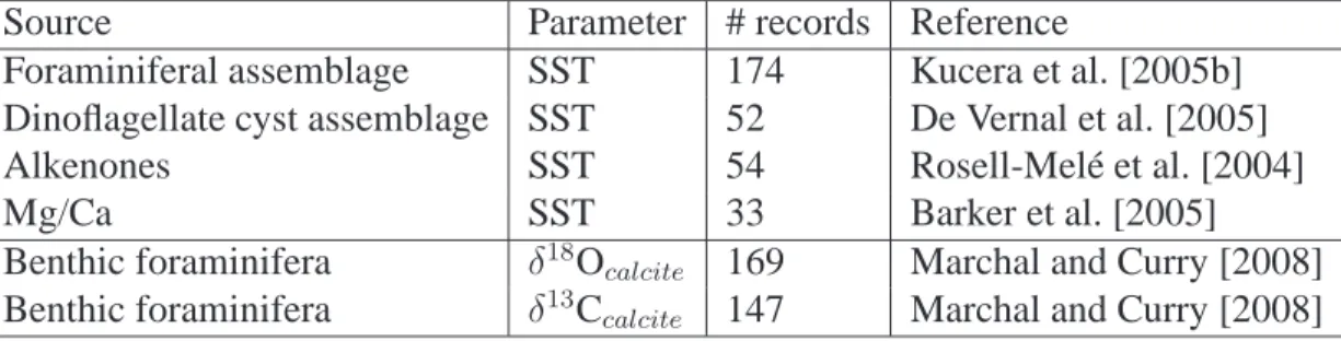
![Figure 2-5: An adaptation of Figure 2 from De Vernal et al. [2006]. Reconstructed annual mean NSSTs at the LGM based on planktonic foraminifera and dinocysts](https://thumb-eu.123doks.com/thumbv2/123doknet/14117799.467199/52.918.139.782.139.468/figure-adaptation-figure-vernal-reconstructed-planktonic-foraminifera-dinocysts.webp)