Asymptotic approximations to the error probability for detecting Gaussian signals.

ASYMPTOTIC APPROXIMATIONS TO THE ERROR PROBABILITY FOR DETECTING GAUSSIAN SIGNALS

by

LEWIS DYE COLLINS

B.S.E.E., Purdue University (1963)

S.M., Massachusetts Institute of Technology

(1965)

SUBMITTED IN PARTIAL FULFILLMENT OF THE REQUIREMENTS FOR THE DEGREE OF

DOCTOR OF SCIENCE

at the

MASSACHUSETTS INSTITUTE OF TECHNOLOGY June, 1968

Signature of Author . . . . Department of Electrical Engineering, May 20, 1968

Certified

by

.

_{- ...}

Thesis Supervisor

Accepted by . .. · · · r

Chairman, Departmental Committee on Graduate Students

Archives

ASYMPTOTIC APPROXIMATIONS TO THE ERROR PROBABILITY FOR DETECTING GAUSSIAN SIGNALS

by

LEWIS DYE COLLINS

Submitted to the Department of Electrical Engineering on May 20, 1968 in partial fulfillment of the requirements for the Degree of Doctor of Science.

ABSTRACT

The optimum detector for Gaussian signals in Gaussian noise has been known for many years. However, due to the nonlinear nature

of the receiver, it is extremely difficult to calculate the probability

of making decision errors. Over the years, a number of alternative performance measures have been prepared, none of which are of universal applicability. A new technique is described which combines "tilting" of probability densities with the Edgeworth expansion to obtain an asymptotic expansion for the error probabilities.

The unifying thread throughout this discussion of performance is the semi-invariant moment generating function (s). For the problem of detecting Gaussian signals, (s) can be expressed in terms of the Fredholm determinant. Several methods for evaluating the Fredholm determinant are discussed. For the important class of Gaussian random processes which can be modeled via state variables, a straightforward

technique for evaluating the Fredholm determinant is presented.

A number of examples are given illustrating application of

the error approximations to all three levels in the hierarchy of

detection problems, with the emphasis being on random process problems. The approximation to the error probability is used as a performance index for optimal signal design for Doppler-spread channels subject to an energy constraint. Pontryagin's minimum principle is used to

demonstrate that there is no waveform which achieves the best perform-ance. However, a set of signals is exhibited which is capable of near optimum performance. The thesis concludes with a list of topics

for future research.

THESIS SUPERVISOR: Harry L. Van Trees

3

ACKNOWLEDGMENT

I wish to acknowledge the supervision and encouragement of my doctoral research by Prof. Harry L. Van Trees. I have

profited immeasurably from my close association with Prof. Van Trees, and for this I am indeed grateful.

Profs. Robert G. Gallager and Donald L. Snyder served as readers of this thesis and their encouragement and suggestions are gratefully acknowledged. I also wish to thank my fellow graduate students for their helpful suggestions: Dr. Arthur Baggeroer,

Dr. Michael Austin, Mr. Theodore Cruise, and Mr. Richard Kurth. Mrs. Vera Conwicke skillfully typed the final

manuscript.

This work was supported by the National Science

Foundation and by a Research Laboratory of Electronics Industrial Electronics Fellowship.

TABLE OF CONTENTS

Page

A. The Detection Problem 11

B. The Gaussian Model 12

C. The Optimum Receiver 13

1. The Estimator-Correlator 16

2. Eigenfunction Diversity 18

3. Optimum Realizable Filter

Realization 20

D. Performance 22

CHAPTER II APPROXIMATIONS TO THE ERROR PROBABILITIES

FOR BINARY HYPOTHESIS TESTING 26

A. Tilting of Probability Distributions 26 B. Expansion in Terms of Edgeworth Series 34

C. Application to Suboptimum Receivers 40

D. Summary 45

CHAPTER III GAUSSIAN SIGNALS IN GAUSSIAN NOISE 46 A. Calculation of (s) for

CHAPTER IV

CHAPTER V

B. Transition from Finite to Infinite

Set of Observables C. Special Cases

1. Simple Binary Hypothesis, Zero Mean

2. Symmetric Binary Problem 3. Stationary Bandpass Signals

D. Simplified Evaluation for Finite

State Random

Processes

E. Semi-Invariant

Moment Generating

F. Summary

APPROXIMATIONS TO THE PROBABILITY OF ERROR FOR M-ARY ORTHOGONAL DIGITAL COMMUNICATION

A. Model

B. Bounds on the Probability

of Error

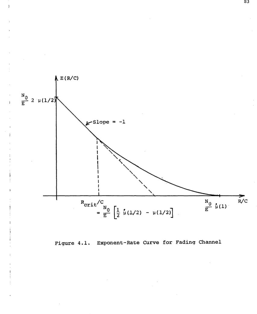
C. Exponent-Rate Curves

EXAMPLES

A. General Binary Problem, Known Signals,

Colored Noise

B. Slow Rayleigh Fading with Diversity

1.

Simple Binary Problem,

Bandpass Signals

2.

Symmetric Binary Problem,

3. The Effect of Neglecting Higher Order Terms in the Asymptotic Expansion 4. Optimum Diversity

Page

Page

5. The Inadequacy of the

Bhattacharyya Dis tance

99

6. The Inadequacy of the

Kullbach-Leibler Information Number as

a Performance Measure 101

C. Random Phase Angle 105

1. Simple Binary, No Diversity 105 2. Simple Binary, With Diversity 110 D. Random Process Detection Problems 114

1. A simple Binary (Radar) Problem,

Symmetric Bandpass Spectrum

117

2. A Symmetrical (Communication)

Problem, Symmetric Bandpass

Spectra 120

3. Optimum Time-Bandwidth Product 124 4. Long Time Intervals, Stationary

Processes (Bandpass Signals,

Symmetric Hypotheses)

124

5.

Pierce's

Upper and Lower Bounds

(Bandpass, Binary Symmetric)

131

6. Bounds on the Accuracy of Our

Asymptotic Approximation for

Symmetric Hypotheses and Bandpass

Spectra

140

7. A Suboptimum Receiver for

Single-Pole Fading 142

8. A Class of Dispersive Channels 146

9.

The Low Energy Coherence Case

149

CHAPTER VI CHAPTER VII APPENDIX A APPENDIX B APPENDIX C APPENDIX D REFERENCES BIOGRAPHY

OPTIMUM SIGNAL DESIGN FOR SINGLY-SPREAD TARGETS (CHANNELS)

A. A Lower Bound on (1)

B. Formulation of a Typical Optimization Prob lem

C. Application of Pontryagin's Minimum Principle

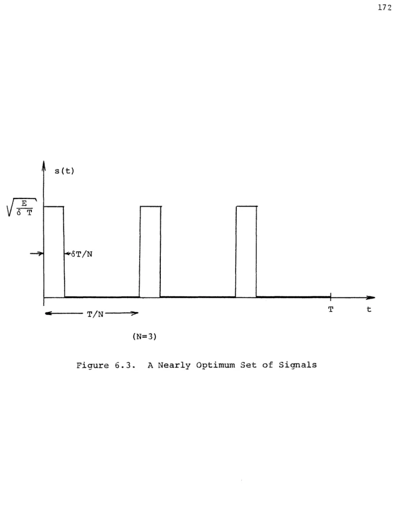
D. A Nearly Optimum Set of Signals for Binary Communication

TOPICS FOR FURTHER RESEARCH AND SUMMARY

A. Error Analysis

B. More than Two Hypotheses

C. Markov (Non-Gaussian) Detection Problems D. Delay-Spread Targets E. Doubly-Spread Targets F. Suboptimum Receivers G. Bandpass Signals H. Summary

ERROR PROBABILITIES IN TERMS OF TILTED RANDOM VARIABLES

p(s) FOR OPTIMAL DETECTION OF GAUSSIAN RANDOM VECTORS

u(s) FOR OPTIMAL DETECTION OF GAUSSIAN RANDOM PROCESSES

REALIZABLE WHITENING FILTERS

7 i Page 154 156 158 162 170 178 178 178 179 180 181 181 181 181 185 192 198 205 213 221

8

LIST OF ILLUSTRATIONS

Page

1.1 Form of the Optimum Receiver 14

1.2 Estimator-Correlator Realization 19

1.3 Eigenfunction Diversity Realization 19 1.4 Optimum Realizable Filter Realization 21 2.1 Graphical Interpretation of Exponents 33 3.1 State-Variable Random Process Generation 62

3.2 A Class of Suboptimum Receivers 69

3.3 Suboptimum Receiver: State-Variable 73 Model

4.1 Exponent-Rate Curve for Fading Channel 83 5.1 Bounds and Approximations for

Known Signals 89

5.2

Approximate Receiver Operating Characteristic,

Slow Rayleigh Fading 93

5.3 Error Probability for Slow Rayleigh Fading

with Diversity 96

5.4 Optimum Signal-to-Noise Ratio per Channel,

Slow Rayleigh Fading 98

5.5 p(s) Curves for Two Diversity Channels 102

5.6 Receiver Operating Characteristic,

Random Phase Channel 111

5.7 Receiver Operating Characteristic, Random

Phase Channel, N 1 115

5.8 Receiver Operating Characteristic, Random

9

Page 5.9 Approximate Receiver Operating Characteristic,

Single-Pole Rayleigh Fading 121

5.10 Probability of Error, Single-Pole Rayleigh

Fading 123

5.11 Optimum Time-Bandwidth Product, Single-Pole

Rayleigh Fading 125

5.12 Optimum Exponent vs. Signal-to-Noise Ratio,

Single Square Pulse, Single-Pole Rayleigh 126 Fading

5.13 Optimum Signal-to-Noise Ratio vs. Order of

Butterworth

Spectrum

129

5.14 Optimum Exponent vs. Order of Butterworth

Spectrum

130

5.15 Single-Pole Fading, Suboptimum Receiver 143

5.16 Tapped Delay Line Channel Model 147

5.17

u(s) for Three Tap Channel

150

6.1 Communication System Model 155

6.2 General Behavior of Optimum Signal 167

6.3 A Nearly Optimum Set of Signals 172

6.4 Optimum Exponent vs. kT, N Samples,

Single-Pole Fading ₁₇₄

6.5 Optimum Exponent vs. kT, Sequence of Square

Pulses, Single-Pole Fading ₁₇₆

D-1 Realizable Whitening Filter 206

.Lo

DEDI CATION

This thesis is dedicated to

i.L

I. INTRODUCTION

In this chapter, we give a brief discussion of the detection

problem. We briefly

review the form of the optimum receiver and

motivate the discussion of performance which occupies the remainder of

this thesis.

A. The Detection Problem

We shall be concerned with a subclass of the general problem which statisticians for a couple of centuries have called "hypothesis

testing" [1-31. Since World War II this mathematical framework has been applied by engineers to a wide variety of problems in the design

and analysis of radar, sonar, and communication systems 4-71. More recently it has been applied to other problems as well, such as seismic detection.

The general mathematical model for the class of problems that

we shall consider is as follows:

We assume there are M

hypotheses

Hi, H2, a.. , HM which occur with a priori probabilities P1,

p

PM On the j hypothesis the received waveform is:

j:r(t) = sj(t) + m(t) + w(t), T < t T (1.1)

where s(t)

is a sample function

from

a zero

mean

random

process

having finite power, mj(t) is a known waveform, and w(t) is a sample function of zero mean white noise.

Our goal as engineers is to design and build efficient detection systems. We shall be concerned with the issue of how well

12

are all related to the error

probabilities:

Pr [ I] = Pr[an incorrect decisionjH.1 (1.2)

The bulk of this thesis is concerned with the issue of computing these

probabilities.

Detection problems may be logically divided into three broad

categories in order of increasing complexity. The simplest category is

detecting the presence of a known waveform in additive noise.

The

next level of difficulty treats those problems in which the signal

waveform is known, except for a finite number of random (unwanted)

parameters. Finally, there is the problem of detecting sample functions

of random processes.

Here the "'signal" is an unknown waveform about

which our only knowledge is statistical

in nature. Equivalently, we

may think of it as a signal with an infinity

of unknown parameters.

In all that follows we shall concentrate on this last category because

the erformance problem is unsolved except for a few special cases. B. The Gaussian Model

In much of what follows we choose to model the signal and noise waveform as sample functions from Gaussian random processes. The first reason for this is purely for mathematical convenience since

this assumption enables us to completely characterize the random

processes without an undue amount of complexity.

The second reason,

being a physical one, is of greater consequence from an

engineering

point of view. First of all, many of the additive disturbances which corrupt real-world detection systems indeed do have a Gaussian

13

distribution. For example, the shot and thermal noise arising in an amplifier or the solar and galactic noise picked up by an antenna

fit the Gaussian model very well [8-9]. Secondly, the random signals which we are interested in detecting are often well modeled as sample functions from Gaussian random processes. For example, the signals received over several types of fading radio channels have been observed in many independent experiments to obey Gaussian statistics [10-11].

C. The Optimum Receiver

The structure of the optimum receiver is well-known [12-131 so we shall not dwell upon it. For a number of detection criteria the optimum receiver computes the likelihood ratio or some monotone function of it, such as the logarithm. This number is then compared with a threshold whose value depends uon the criterion chosen. For

the M-hypothesis problem, the optimum receiver consists of M-1

branches each of which computes a likelihood ratio or some equivalent test statistic.

For most of this thesis, we restrict ourselves to the binary (i.e., M = 2) problem in the interest of simplicity. In Chapter IV we shall discuss the generalization of our results to the more general M-ary problem.

The most general form of the optimum processor under our Gaussian assumption consists of a linear and a quadratic branch as indicated in Fig. 1.1. In this figure, the output random variable is the logarithm of the likelihood ratio A (r(t)).

14 ,) U ,) 0 a) EE 0 4I-q 4i

0

_r

15

There are several equivalent forms of the optimum processor, some of which we shall encounter as we proceed with our work. Here we briefly

review these optimum receiver realizations. For derivation and more detailed discussion, see Van Trees 13]. For simplicity in our brief

discussion, we shall discuss only the simple binary detection problem:

H

: r(t) = s(t)

+

w(t)

T.< t < T

(1.4)

H1: r(t)

=

w(t)

where s(t)

is a sample function

from a zero mean Gaussian random

process with covariance K

(t,

r),

and u(t) is a sample function

of

zero-mean white Gaussian noise with spectral density N0/2.

For the problem that we have outlined, the log-likelihood ratio may conveniently be broken into two parts, a random variable and a constant term (the "bias") that is independent of the received

data.

R + B (1.5)

9

_{R depends on the received data and}

ZB = aZn(l + 2X.i/N) (1.6a)

i=l

= n 1 (1 + 2XiNo (l.6b)

16

where {X

are the eigenvalues of the homogenious Fredholm integral

equation,

Tf

xi

i(t) = f

Ti

Ks (t,T)i(T)dt,

i-

In integral equation theory, infinite products of the form in Eq. 1.6b are called Fredholm determinants. We shall define the Fredholm determinant to be,

D (z) =fi

i-l

(l+zAi) .

(1.8)

This function occurs repeatedly in our performance calculations and we shall develop closed-form techniques for evaluating it in

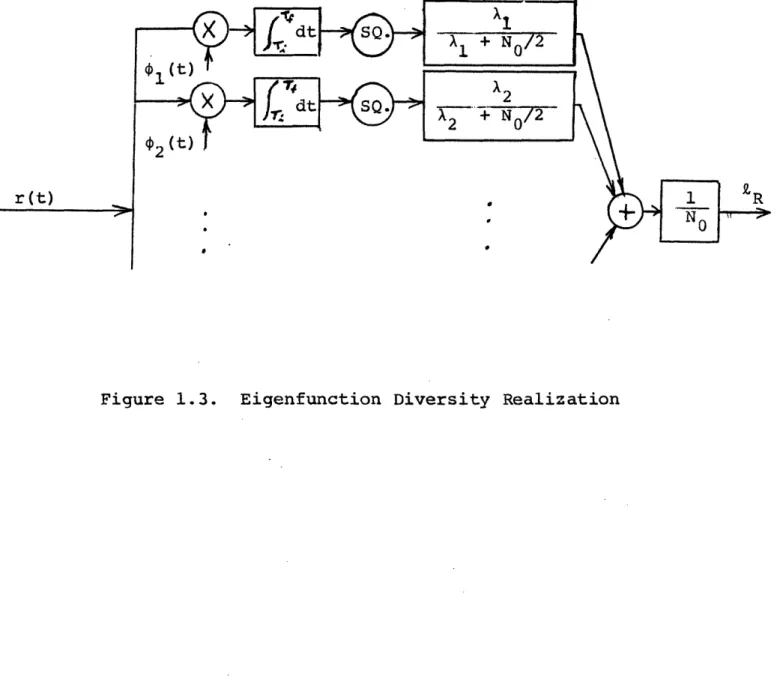
Chapter III. We now shall discuss techniques for generating _.R 1. The Estimator-Correlator. Price [12] originally derived the intuitively pleasing realization of Fig. 1.2,

R NO | T

Tf

Ti

T

(1.7)

17

r(t)

18

where

h(t,u) is specified

by an

integral

equation of the Wiener-Hopf

type

Tf

'(tu) = 0-itu) K (t5, )h(,u)dt T < t, u < T

S 2 I -' --

T

(1.10)

We immediately recognize that h (t,u) is the impulse response of the optimum MMSE unrealizable linear filter for estimating s(t), given r(t) =

s(t) + u(t), T_i < t < Tf' Hence, from Eq. l.9b

Tf

ZR No f rt)s(tT)dt (1.11)

Ti

where s(te Tf) denotes the unrealizable estimate of s(t). Thus, the receiver performs the familiar correlation operation, where we correlate with the best (MMSE) estimate of the signal.

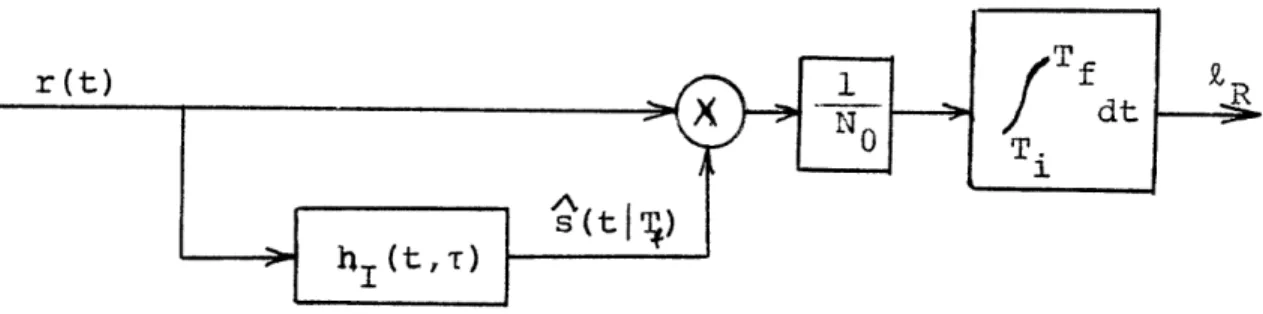
2. Eigenfunction Diversity. A second realization which is useful from a conceptual point of view is that shown in Fig. 1.3. It follows immediately from the Estimator-Correlator if we exapnd r(t) and hI(t,u) in the eigenfunctionsof s(t).

2

1 A.r.

N

Figure 1.3. Eigenfunction Diversity Realization

19

20

Equivalently, the estimator-correlator can be (and usually is) derived from Eq. 1.12. We shall find it useful to make use of the observation from this realization that RR in the sum of squares of statistically independent Gaussian random variables.

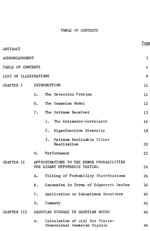
3. Optimum Realizable Filter Realization. A third realization due to Schweppe [141 is shown in Fig. 1.4.

Tf

R

NoJ

T

This realization

has the advantage that the

linear

filter

is

realizable.

It satisfies the linear integral equation,

N t KS(t,u) = O ho(t,u) +/ T. 1 Ks(t,¶)ho(T,u)dT, Ti. < u < t < Tf, (1.15)

which is frequently easier to solve than Eq. 1.10.

This realization is of particular importance when s(t) can be modeled as the output of a linear dynamic system which is driven with white Gaussian noise. Then the techniques of Kalman-Bucy

21

r

(t)

filtering

[15] enable us to find s(ti t) as the output of a second

dynamic system. We shall return to this class of problem in

Chapter III.

D. Performance

A problem which is closely related to that of determining

the optimum receiver is the question of evaluating its performance.

We would like to be able to do this for two reasons:

(1) to enable

us to pick the setting of the threshold on which the decision is based;

and (2) to evaluate and compare various detectors.

In designing a digital communication system, one most

frequently desires to minimize the total probability of error

Pr[e]

-

Pr[c1H]Pr[H

1

+ Pr[IH

]Pr[H

].

(1.16)

On the other hand, in radar and sonar problems it is common

practice

to employ a Neyman-Pearson criterion

[2] in which the probability

of a false alarm, P, is constrained; and we desire to minimize the

probability of a miss, PM,

PF

Pr[e|Hl]

(1.17)

PM = Pr[cH 2]. (1.18)

Another performance measure of this same type is the Bayes cost,

C CFPF + CMPM'

22

23

where C

and CM denote the costs assigned to a false alarm and miss,

respectively.

The problem of

computing

the output

probability

distribution

of

a nonlinear

detector, such as shown in Fig. 1.1, has been studied

for over twenty years [16-20].

The basic technique is to compute the

characteristic function of the output random variable in terms of the

eigenvalues of a suitable eigenfunction expansion.

Only recently

has a satisfactory

technique for finding the eigenvalues become

available [21]. We thus can approximate the characteristic function

by using the most

significant

eigenvalues.

However,

we

then are

faced with the computational problem f evaluating (numerically) an

inverse Fourier transform. Although highly efficient algorithms exist [22], the constraint of computer memory size makes it difficult to obtain sufficient accuracy on the tail of the probability density.

Perhaps the most widely used measure of detector

perfor-mance

is

the "output signal-to-noise

ratio."

This terminology

certainly has a physical, intuitive appeal from an engineering point

of view.

As commonly defined,

the output signal

to

noise

ratio

depends only on the first and second moments of the receiver output,

2 [E(LH 1) - E(LIH2)12

d2 = - (1.20)

24

Therefore, the ease of computing d contributes to its popularity.

However, since two moments do not completely characterize

the

probability distribution of the test statistic in most cases, this

performance measure is not of universal applicability.

Two important examples when

d

is an adequate performance

measure are the known signal detection problem and the "low energy

coherence" or "threshold" case in which the signal energy is spread

among a large number of coordinates [23].

Then the error

proba-bilities

can be expressed in terms of the Gaussian error function.

P.

z

d

PM 1

(2

(1.21b)

x l

where

(x)

1

exp -

dy.

(1.22)

(-7 2

The simplest distance measures are the Kullback-Leibler

information numbers [24].

I(H1:H 2) = -E[IH 1

1

I(H

:H

) = E[LjH

]

(1.23b)

The divergence [25] is related to the Kullback-Leibler information numbers and may also be regarded as an unnormalized

25

J I(H₂:H₁) + I(H₁:H2) (1.24a)

- E(ZIH 2) - E[)

1H]

The Bhattacharyya distance 26] has been proposed as an alternative performance measure which is of wider applicability

than d2 or the divergence.

B -n ... (prH (R) prH (R)] dR

- r-H₂

- -en EA2{H_{] 1}

_1

- -n E[A

21.

This distance measure is sometimes referred to as the Kakutani [27]

or Hellinger [281 distance.

Kailath recently discussed these last two performance

measures [29]. In Chapter V, we shall give simple counterexamples where these performance measures give misleading results because

the ordering of the values of the performance measure doesn't always

correspond to the same ordering of the error probabilities.

Therefore,

we shall conclude that these performance measures should be applied

26

II. APPROXIMATIONS TO THE ERROR PROBABILITIES FOR BINARY HYPOTHESIS TESTING

In this chapter we develop asymptotic approximations to

the error probabilities for detecting random signals.

We first use

the technique of tilted probability distributions to write the error

integrals

in a form well suited to our subsequent application

of the

Edgeworth expansion.

A. Tilting of Probability Distributions

Since exact calculation of error probabilities is in most cases difficult, we shall consider the possibility of approximating the error probabilities in some fashion which is computationally

attractive and which is of sufficient accuracy to be of real value. One possibility is to find upper and lower bounds for the error probabilities. This approach has been successfully employed by the information theorists in proving coding theorems, for example [30]. A second possibility is to make an asymptotic approximation [31] to the error probability which is valid over a range of some parameter such as the signal-to-noise ratio.

The technique that we employ is usually called "tilting" of probability distributions. It was introduced into information and coding theory by Shannon [32] and has been employed with great success. Earlier applications in the field of mathematical statistics are due to Chernoff [33] and Esscher [34]. In this section, we

summarize the notation and results. In the interest of readability, the mathematical details are relegated to Appendix A.

77

Since the log-likelihood ratio may be considered as the weighted sum of statistically independent random variables, a logical

approach to computing its probability density is to consider the characteristic function, which is the product of the characteristic functions of the individual random variables in the sum. Actually, we use the semi-invariant moment-generating. function which is the

logarithm of the conditional moment generating function M H (s).

U(s) - n MHlH (s)

= in f pH2(R) Pl H (R) d(R). (2.1)

For our purposes, it suffices to consider s to be real. Furthermore, Equation 2.1 is valid only over some range of s, say, s < s < s2,

which is the familiar "region of convergence" associated with a

Laplace transform. We shall have more to say about the range of s as we proceed.

It is sufficient to consider only one of the two conditional

characteristic

functions since the two are simply related for the

optimum receiver which makes its decision from the logarithm of the

likelihood ratio.

Note that we have chosen to use the symbol commonly used for the

characteristic

function to denote the moment-generating function.

28

M H (s)

=

(

In the last section of this chapter, we shall present the necessary modifications of our development which enable us to treat suboptimum

receivers.

Straightforward differentiation of Eq. 2.1 yields

~(s)

f Pr

(R) Z(R)dR,

(2.3)

'(s)

=

r (R)Z

(R)dR - [(s)12

(2.4)

which are the mean and variance of Z(R) with respect to the probability density 1-s s rHl H (R) PrH2 (R) Pr (R)

1-s

=

ep[-(s)lp

-s R) P

RH2

(2.5b)

Hence i(s) > 0, with equality occurring only in the

unin-teresting

case when

is a constant with probability

one.

Thus,

u(s) is strictly

convex downward

in all cases of interest to us.

In addition,

(2.6)

V(o) = (1) = 0,

so that

u(s) < 0 for 0 < s < 1.

(2.7)

We refer to pr (R) as the "tilted" density. The amount of -S

"tilting" depends on the value of the parameter s. It follows from our definition that,

(R) = Pr (R) exp[p(s)-sZ(R) ,

PrIH (R)

P(R)

exD[l(s)+(l-s)(R)j.

(2.8)

(2.9)

Hence, the error probabilities may be expressed in terms of

u(s) and the tilted density Pr (R).

--s

Pr[e H

i]

=

(2.10)

(2.11)

30

where y denotes the threshold level, and p (L) is the tilted

S

probability density for the log-likelihood ratio corresponding to the nonlinear transformation = g( r ) .

At this point, we should perhaps comment on the range of validity of Eqs. 2.10 and 2.11. In general, we can only say that

Eq. 2.1 is valid for 0 < s < 1, since, if either of the conditional

probability densities should vanish on some set of finite measure

the integral would not converge for s < 0 or s > 1. Of course, Eq. 2.1 may be valid for values of s outside of [0,1].

Furthermore, it is only for 0 < s < 1 that the integrands of Eqs. 2.10 and 2.11 both contain a factor which decays exponentially in the range of integration. Presently, we shall see how this behavior enables us to approximate these integrals.

We perhaps should emphasize that up to this point, we have made no approximations. We have just rewritten the error

probabilities in a different form in which we have introduced an arbitrary parameter s. Although it would appear that we have traded a difficult problem for one that is even more complex, we shall see

that this added complexity leads to some useful approximations. A simple, well-known upper bound that follows immediately from Eqs. 2.10 and 2.11 is the Chernoff bound [33,35]. For example, if in Eq. 2.10 we bound exD[-sL] by exp[-sy], then bound

f p,

(L)dL

y s

and

Pr( H 11 < exp[u(s)-sy

Pr[eJH21 < exp[p(s)+(1-s)yj.

We can minimize these bounds by proper choice of the parameter s.

(S) = Y

Observing from Eq. 2.3 that

u<0) = E[Pl111 ]

and

(1) E[LIH 2l

then the range 0 < s < 1 corresponds to

E[IH 1] < y < E[LIH].2

Moreover, from Eq.2.4, p'(s) > 0, so that a(s) is a monotone function. Hence, a solution to Eq. 2.14 exists and is unique provided the

threshold

y

lies between the means of the conditional densities

P9IH (L) and IH (L). This condition is usually satisfied in the

applications, since when the threshold lies above or below both

conditional densities, one of the error probabilities will be very

31 ( 2, 12)

(2.13)

(2.14)

(2.15a)

'32

large (greater than one-half in many cases).

As pointed out by Shannon, et.al. 36], the exponents in the Chernoff bounds, Eqs. 2.12 and 2.13, have a simple graphical interpretation. We draw a tangent to the (s) curve at

s = s where (s ) = y. This tangent line intersects the lines s = 0 and s = 1 at (s ) - s (s ) and (s ) + (1-s )(s ), respectively. See Fig. 2.1. Therefore, the intersection of the tangent line with

the vertical lines s = 0 and s 1 are the exponents in the

Chernoff bounds.

Let us digress briefly to point out that all the commonly used "distance measures" can be calculated from the semi-invariant moment generating function (s).

From Eqs. 1.23 and 2.15, the Kullback-Leibler information numbers are

I(H₁:H₂) = -(0), (2.17)

and

I(i2: H1) = (1). (2.18)

The divergence follows immediately from Eq. 1.24.

33 33 -K n -

4-r.

a

4

,j

34

The output signal-to-noise ratio is only slightly more

complex.

Using Eqs. 2.3 and 2.4 in

1.20,

we have

d2 (l) - (0) 2 (2.20)

Finally, from Eq. 2.1, we see that the Bhattacharyya distance is just one point on the (s) curve.

B= -Ln ... $ (R) p (R) dR

VPr[H2

-

'H1

(2.21)

B. Expansion in Terms of Edgeworth Series

A simple example of an asymptotic expansion for error probabilities is provided by the known signal in Gaussian noise

problem. A well-known asymptotic power series for the Gaussian error function Eq. 1.22 is

1

-

(x)(

xp2x

x

+ ....

(2.22)

The first term of this series is an upper bound which becomes extremely tight for moderately large values of x.

1 - (x) < 1 exp( - 2 (2.23)

35

Either of the above results can be used in Eqs. 1.21a and 1.21b to obtain approximations to PF and PM. In this section we generalize these notions to our more general problem. We now derive an asymptotic expansion for the error probabilities in the general case. For simplicity in all that follows we shall treat only Pr[eIH1]. The derivation for Pr[eH 2] is very similar.

First, we introduce a normalized, zero-mean random variable

i - )

z = . (2.24)

(s)

Then,

Pr[lIH

]

-

exphl(s) -

s(s)]

f

esv

p()

PZ

(Z)dZ.

(2.25)

0 s

Before proceeding from Eq. 2.25, let us point out the motivation for introducing the tilted random variable 9. (and subsequently Zs).

One of the serious practical problems which we encounter in the straightforward evaluation of the error probability is that we are generally interested in the behavior far out on the tail of the probability density. Since the test statistic is made up of a large number of statistically independent components, we would like to apply

the Central Limit Theorem. However, this theorem is of little use when the region of interest is the tail of the probability density.

But observe that in our alternative error expression, Eqs. 2.10 and 2.11, we no longer are integrating under the tail of a .:-1

36

probability density, but rather we start integrating at the mean of the tilted variable . Furthermore, the integrand contains a

decaying exponential factor which results in the value of the integral being determined primarily by the behavior of p (L) near the mean

S

rather than on the tail. Thus, we expect, at least heuristically, that the Central Limit Theorem may be used in approximating the error probabilities.

Unfortunately, in most cases of interest p (L) does not

s

tend to a Gaussian distribution

in the limit as the number of

independent components goes to infinity.

This is a consequence of our

covariance functions being positive definite, square integrable

functions

from

which it immediately follows that the variance of

s

remains finite as the number of independent components goes to infinity. In this case, a necessary and sufficient condition that p (L)

approaches

the

Gaussian

density

is

that each component random variable

in the sum be Gaussian [38], which is not the case except in the

known-signal detection

problem.

However,

experience

has shown us that

the limiting distribution,

while not converging to the Gaussian

distribution, does not differ a great deal from the Gaussian. Therefore, it is fruitful to make an expansion of pz (Z) which is related to the

s

Gaussian distribution. Such an expansion is the Edgeworth expansion, the first few terms of which are given below [39].

Pz (Z) (Z) - [ 6 (3) (Z

2

V.-37 2 Y5 +(5)

_(z)

₊

₄

₊

_Z

_{+ Y (6zi}

_{4 +(8)(z)}

₊

_{(z) 8}

1

+ 1728

()

+ 31104

(Z)

dk

This expansion may be obtained from a Hermite expansion of p (Z) (also sometimes called a Gram-Charlier series) upon reordering the terms. It has the further advantage for our purposes that the coefficients are expressed in terms of the semi-invariants of the random variable zs, which are readily computed from (s).

We

now

substitute the Edgeworth expansion into the integral

in Eq. 2.25 and interchange orders of integration and summation. We then are faced with the task of evaluating integrals of the form

38

(2.29)

Repeated integrations by parts enable us to express these integrals in terms of the Gaussian error function

+(X) = 1 exp - dZ.

- /

2

The first few integrals are:

2

I

(a)

=

(-a) exp(2 )

Ii(a) = a 10(9)

I(a)

a2

O(a)

-12( a IO)

-I3 (a) = 3 0(a) + 1 2 )

I₄(a) = ac₄ I(a) + 1 (a - a3)

I5(a) ab I0(a) + 1 (-3 + 2 _ 4) I6(a ) = 6 I 0() + (-3a + a3 aS).

(2.30)

(2.31c)

(2.31g)

Ik(a

-

j

~

(Z) exp(-aZ)dZ.

39

.jy

Thus, we have our approximation to Pr[EcH1]. We simply evaluate u(s) and its derivatives then substitute. This procedure is far too complex

to be used analytically, but if we use a digital computer to obtain a(s) as we must in many problems then there is no disadvantage in having the computer evaluate our error approximation as well.

We shall frequently retain only the first term in Eq. 2.26 in the asymptotic expansion of the integral in Eq. 2.25. Then,

Pr[IH _l] (-s/ i(s) )expzu(s) - s i(s) + (s). (2.32)

Similarly, we obtain

Pr[EH2] Z

(-(l-s)

i(s)

)exp|j (s)+(l-s)

(s)

+

2

'

s)

(2.33)

Higher order approximations to the error probabilities are obtained in the same fashion. For example, the second order

approximation

to

Pr[cH

follows from retaining the first

two

terms

in Eq. 2.26 and using Eqs. 2.31a and 2.31d. The result is,

Pr[ H

] exp[1(s) -

s(s)]

0(

i

-s

)ex

)(l -

s

S)

L

_{L~~~___}

-i)

'2

(

(ls

s))

- '<Fy3/

40)

A further approximation results from using the asymptotic power series, Eq. 2.22, for the Gaussian error function in the above equation. Then Eq. 2.32 becomes,

PrHI

Hlj

=1

expbp(s)

-

s(s)],

(2.35)

v2rsii(s)

and after making some cancellation, Eq. 2.34 becomes

Pr[H

]

/ 2r $2j(s) s]Z/ (s j

(2.36) Similar expressions result for Pr[EH2 .

It should be pointed out here that we have not used the Gaussian assumption on the received signals up to this point. In the next chapter, when we actually compute i(s), we shall make use of this assumption to obtain closed-form expressions. Furthermore, observe that Eqs. 2.32 and 2.33 are the same approximations which would result if we were (in most cases incorrectly) to apply the Central Limit Theorem to Eq. 2.25.

C. Application to Suboptimum Receivers

In many situations it is convenient for either mathematical or physical reasons to use a suboptimum receiver. Although our

techniques are best suited to the analysis of optimum receivers because of the property given in Eq. 2.2, we frequently may want to

I'

consider suboptimum receivers. For example, instead of building a time-varying linear estimator followed by a correlator, we may choose to use a time-invariant filter followed by an envelope detector, as is frequently done in practice. We would like to investigate how our approximation can be adapted to such problems. On the basis of

previous experience, we suspect that suboptimum systems can be found which work very well. In this section, we develop the necessary

modifications to allow us to approximate the error performance of such

suboptimum receivers.

Since this development differs

somewhat from

the usual case where the test statistic

is the logarithm of the likelihood

ratio, we shall include the details.

Since Eq. 2.2 no longer holds, we must treat the two

hypotheses separately.

First, consider

H

Our development closely

pl(s) Ain M | H (s) (2.37)

where we no longer require that

PrjH (R)

Z = n A(r) in (238)

H

P (R)

Now we define a new tilted

random variable

is

to have the

probability density

sL - U(s)

42

Then,

Pr[CIH

]

'V Is

where once again y denotes the threshold level. Just as before, we expand p (L) in an Edgeworth expansion. Therefore, we shall need

ls

the semi-invariants of the titled random variable ils

tL ls -

£n

/

e(+t)L

-

l(S)

l(S)

k

and the coefficients in the Edgeworth expansion of p (L) are obtained from the derivatives of Pl(S) just as before.

Similarly, under H,2

2(s) a n MH (s). (2.43)

sL -

2(s)

2s

(s)

-

sL

en M2 (t)

(

s) - U2(s)

and the semi-invariants

of 2s are,

k

k u2(s)

which appear in the Edgeworth expansion of p

Our bounds and approximations

follow immediately from

Eqs. 2.10 and 2.11.

The Chernoff bounds are:

Pr[E H

< exp[p

i(sl)-slyJ

for

s

>

0

(2.47)

Pr[sIH

exp[p

(s

)-s

Y

for

s2

< 0.

(2.48)

The first-order approximations are,

(2,44)

(2.45)

(2.46)

(L).

i2s

P' 4 4 where 2 Pr[cH ₂l] X~ (+s2_2* xi₂ 2(s_{2 2} 2))exp[p2₂ (s_2~~T 2)-s2j2(s2)+ 2 _{'2 2} (2.49)

(2.50)

(2.51)

and

Since,

l(S) and u

(s) are monotone increasing functions of s. Then,

Eq. 2.51 has a unique solution for s > 0 if,

Y > '1(0) E[ iH1

and Eq. 252 has a unique solution for s <

if

< 2(o) E[ZIH21.

(2.52)

(2.53)

(2.54)

(2.55)

(2.56)

r

E[H 1] < E[Z jH2 (2.57)

in order to be able to solve Eqs. 2.51 and 2.52. D. Summary

In this chapter, we have developed several bounds on and approximations to the error probabilities for a rather general binary detection problem. The semi-invariant moment generating function u(s) played a central role in all our results. These results were obtained without making any assumptions on the conditional statistics of the received signals. In the next chapter we evaluate u(s) for the specific class of Gaussian random processes.

r

46

III. GAUSSIAN SIGNALS IN GAUSSIAN NOISE

In this chapter, we make use of the Gaussian assumption on the received signals to obtain closed-form expressions for the semi-invariant moment generating function (s) in terms of minimum mean-square estimation errors. In the important case when we can model our random processes via state variables, this calculation is particularly straightforward.

A. Calculation of p(s) for Finite-Dimensional Gaussian Signals As a first step in obtaining (s) for the general Gaussian binary detection problem, we consider a related problem from the second level in our hierarchy of detection problems.

Hi: r s₁ + m + w

H2 r s2 + m2 + , (3.1)

where s and s₂ are N-dimensional zero-mean Gaussian random vectors with covariance matrices K and K , respectively; m and m2 are

-s1 -2

known N-vectors; and w is a Gaussian random N-vector with statistically independent components each having variance o2. Thus,

w K

H

K

-=K

+a2

I

-K

(3.2b)

r

(

N/

1K

1

We now substitute Equations 3.3a and 3.3b in Equation 2.1 for (s). We make use of the existence of an orthogonal matrix

(i.e., QT = Q ) which diagonalizes the quadratic term in the exponent of the integrand. This enables us to complete the square in the

exponent, making the evaluation of the N-fold integral straightforward. The tedious algebraic details of these calculations appear in Appendix B. The result is .(s) +2 -

2 Qnl(l-s)K

+ slI

48 or

(tI.

+

K

+

ni

-l

a

2

2

+W

( ) +

₂

-s

2

B. Transition from Finite to Infinite Set of Observables We now make use of the results of the previous section to evaluate (s) for the general Gaussian binary detection problem.

Hl:r(t) l(t) + m(t) + w(t),

T < t < Tf, (3.5)

H₂:r(t) - s₂(t) + m₂(t) + w(t),

where sl(t) and s2(t) are sample functions from zero-mean Gaussian random processes with known covariance functions Kl(t,T) and K₂(t,T), respectively; m(t) and m2(t) are known waveforms; and w(t) is a sample function of white Gaussian noise with spectral density N0/2.

We choose the components of r to be N uniformly spaced time samples of the random process r(t). We then let the sampling become dense; that is, we let N + . From Fredholm integral

r

equation theory we are able to express the first three terms in

Eq. 3.4b as Fredholm determinants of appropriate covariance functions. The last term in Eq. 3.4b in the limit can be expressed in terms of

the solution to a non-homogeneous Fredholm integral equation. We

relegate the details to Appendix B and state the results here.

(s) = Z Zn(l + 1 ) + Zn(l + i2 i=l0 i= 0

_

E

Zn(l

+

-A

)

where {Ail} and {Xi2} are the eigenvalues of Kl(tT) and K2(t,), respectively; and {mi1} and {mi2} and the coefficients of ml(t)

and m2(t) when expanded in terms of the eigenfunctions of the

composite random process s (t). comp

KComp(t,r:s) = (l-s)K2(t,T) + sKl(t,r). (3.7)

The first three terms in Eq. 3.6 are all Fredholm

00

Df(Z)

=

ff

(+XZ)

(3.8)

i-1

Several closed-form expressions for the Fredholm deter-minant have appeared in the literature. Siegert [20, 40] related

it to the solution of integral equations of the Wiener-Hoof type.

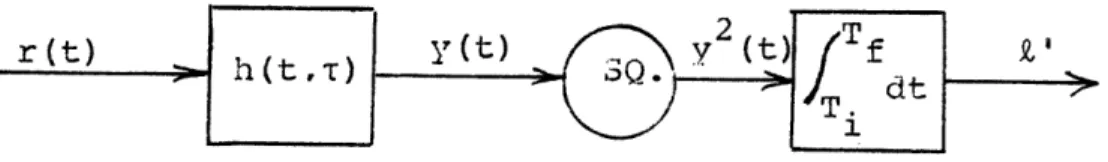
An D (Z) n(l N X (3.9) ._ 2 NO Tf f dz 1 f hi(tt: z)dt (3.10) 0 Ti Tf N = f ho(tt: )dt (3.11)

T.

where h(tT: -) and h(t,T: -2) are impulse responses for optimum minimum mean-square error linear filters (unrealizable and realizable,

respectively) for estimating the random process y(t) when the

observations have been corrupted by additive white noise with spectral height N0/2.

Since the minimum mean-square estimation error is related to the impulse response of the optimum linear filter [41],

N N N

(t

:2)

-

h

(tt

2

(312)

N_O N_O N

yo 2 2 0 2t(3.13)

we have two alternate expressions for the Fredholm determinant.

2 NO T 2 .B

Qn D N)

'

f

dz

r

y(tITf:

)dt

(3.14)

0 T

i

N

(ti t: -)dt

(3.15)

where y (tjT:

2)

[Ti,ti which are corrupted by additive white noise with spectral density N /2.

Thus, we have our expression for (s) in terms of quan-tities which can be readily computed.

Ss)

N~

=

T

,(

1

i

52 Tf N

1-s

f

0

2

T

i

s2

2 Cop tlt: 2,s)dt

T

s(1-s)

m2(t ml()

Ticomp

ES

,

and ScoMp denote the minimum mean-square linear

-'s Sl(t) + 1-8 s2(t), respectively, when observed over [Tit] in additive white noise of spectral height N₀/2. hcomp(t,T:s) denotes

the minimum mean-square linear estimator for estimating the composite process s (t). The last term in Eq. 3.16 can also be interpreted

comp

as d2 (s), the output signal-to-noise ratio for the problem of comp

deciding which of the known signals ml(t) or m₂(t) was sent when observed in colored Gaussian noise with covariance

Kn(t, : 8)

KComp(t,:s) +

N

" s Kl(t,T) + (l-s)K₂(tT) + d6(t-T). (3.17)

An alternate way of writing Eq. 3.16 results from using Eq. 3.15 and the observation that the last term in Eq. 3.16 is an appropriately defined "signal-to-noise ratio".

2

~-s

U(s) 2

Q

s

+

n D2 (-)

2

2 1 N0 2 n s N

-1 n 2 s-s) s( d2 (s) (3.18)

2 .comp Se2 comp

C. Special Cases

There are several special cases of Eq. 3.16 which deserve a few additional comments, particularly since many of the

applications fall into these cases. For these cases, one frequently can derive the expression for (s) in much a simpler fashion. We do not include these simplified derivations here.

1. Simple Binary Hypotheses, Zero Mean. For this problem, only white noise is present on H.

H2:r(t) - s(t) + w(t)

T < t < T

_i

_f

H₁:r(t)

.-53

r

54

The "composite

random process is now

the

same as the 'signal"

random

process, except for the power level. Then,

Tf ii~s) 2 - s(tIt ' ) d N 2 N

0

I

dTi

(tIt:

2 )dt

-

N

₀

O

Ti

i

= [ (1-s)n

N-)

((1-s)

In terms of the eigenvalues of s(t),

00 W~~~~~~0

1

Z:

2(-s)X1

P(s) =

I-s)

i N- i= N0

i~~~l i-l~

~:i

(3. 20a)

(3. 20b)

(3.20c)

We can also obtain closed-form expressions for ;i (s) for this case. Differentiating Eq. 3.21, we obtain

1 2 .

P(s)

₂

-_

- n(l+

)

i1

1

)dt

(tIT

f2(l-s)

j

The second term in Eq. 3.22b is an unrealizable minimum-mean-square filtering error.

Thus, we have closed-form expressions for the exponents in our bounds and approximation.

p(s) + (-s),(s)

Tf

(

(l-

s

_r

Nt

N

dt

(3.22a)

Tf

i

56

f N N

lA(s)-s(s)f 2

[(ti

:-)

(ti

)

Tf N N

+

f

[(-s(

s

t:2()-s)

(3.24)

2. Symmetric Binary Problem. Now consider the symmetric

binary problem where

H1:r(t)

s(t) + w(t)

T_i < t < Tf (3.25)

H2:r(t) = s2(t) + w(t)

We assume that l₁(t) and s2(t) have the same eigenvalues, with the corresponding eigenfunctions being orthogonal. This situation can occur in practice, for example, when s₂(t) is a frequency-shifted version of sl(t), as in an FSK system operating over a fading channel.

From Eq. 3.16

12 D() ) - 2 (l-s))

(s) = 2 - i D -) s -n D ) (3.26)

sy 2 'TNQ _{O O O~~~~~~}

57

Recall that

lSI()

D 2

2(l-s))

PSI (s) if (-s) In D

(-

I 0 7

where "SI" denotes "simple binary".

PS(s)

'

PSI(s) + pSI(l-s)

(3.27)

Thus,

(3.28)

This equation enables us to compute (s) and all its

derivatives for the symmetric problem from those for the simple binary

problem. In particular,

'Psy (1)

2'PS (1

0

1

(3.29a)

(3.29b)

(3.29c)

the signals of

Stationary Bandpass Signals.

In many applications,

interest

are narrowband around some carrier

frequency

58

where the envelope and phase waveforms, A(t) and (t), have

negligible energy at frequencies comparable to w . Equivalently, we can write s(t) in terms of its quadrature components.

s(t)

-=

-2's(t)

cos

w

t + 1ir's

(t)

sin

w

t.

(3.31)

cl C S C

In some of our examples in Chapter V, we shall want to

consider stationary bandpass random processes which can be modeled

as in Eq. 3.31 over some interval T

< t

Tf, where s (t) and s

(t)

are statistically independent stationary random processes with

identical statistics. For this case, the eigenvalues of the bandpass

random process s(t) are equal to the eigenvalues of the quadrature

components.

Each eigenvalue

of s

(t)

or of s

(t)

of multiplicity

N

is an eigenvalue of s(t)

with

multiplicity2N.

BP

We denote the eigenvalues' of s(t) by (A

}

sC(t)

and s (t) by

{Ai

}.

Then from Eq. 3.9, the Fredholm determinant

for s(t) is

-2

2n(l

+2

2ALP

= 2 n D

?3- 2(t)

N)

= 2 n D s

2

Further, observe that

-

A

t-

E

BP

t

i-I

'.%LP

isl

(3.35)

60

For the zero mean case, it follows from Eq. 3.18 that

-0 0

' 2pL (S: ) (3. 36)

where we have explicitly indicated the signal-to-noise ratio in each

term.

We comment

that the results in this

section

are

not the

most general that can be

obtained for bandpass processes, but they

of properties

and

representations

for bandpass random processes

would

D. Simplified Evaluation for Finite State Random Processes An important class of problems in which we can readily

compute the various terms which comprise (s) is those problems in

which the random processes can be modeled as the output of linear

state-variable systems which are driven by white Gaussian noise.

This model includes all stationary processes with rational spectra as

one important subclass of interesting

problems.

The state variable model allows us to use the results

of

the Kalman-Bucy formulation of the optimum linear filtering

problem

to determine the optimum receiver structure as well as to calculate

P(s) [14-15].

The straightforward way to compute the first

three

terms in Eq. 3.16 is to solve the appropriate matrix Ricatti equation

and then integrate

the result over the time interval

[Ti,Tf]as

indicated.

We assume that the random process y(t) (sl(t), s2(t) or

scomp

(t) for the first, second, and third terms in Eq. 3.16,

respectively)

is the output of a linear system which has a

state-variable representation

and which is excited by zero mean white noise,

u(t); that is

d x(t)

=

F(t) x(t) + G(t) u(t)

(3.37a)

dt

...

.

y(t)

=

C(t) x(t)

(3.37b)

u(t) x(t) y(t)

Figure 3.1. State-variable Random Process Generation

63

E[x(T)x T(T₉1 3 (3.37d)

Eq. 3.15 provides a convenient way of computing the Fredholm determinant when we realize the detector or estimator, for y(tlt: -2) appears explicitly in the realization [131. For the problems at hand, the techniques of Kalman-Bucy filtering give

y(tit: - ) in terms of the solution to a matrix Ricatti equation 151.

N i (tlt: 2 ) C(t)Z(t)C (t) (3.38)

where

dt

We now derive a new expression for the Fredholm determinant which does not require integrating a time function over the interval

[Ti,Tf]. Moreover, we obtain this result in terms of the solution to a set of linear differential equations, as contrasted with the nonlinear set in Eq. 3.39a. These advantages are particularly useful from an

64

analytical

and

computational

point

of

view. In particular,

for the

important case in which Eqs. 3.37a-3.37b are time invariant, which

includes

all

stationary processes with rational spectra,

the

solution

to this set of linear differential equations can be written in

closed-form in terms of a matrix exponential. This matrix exponential

is frequently easier to compute than integrating the differential

equation directly.

We start with Eq. 3.15 and then make use of the linear system of equations which is equivalent to Eq. 3.39a [15].

dt l(t) F(t)jl(t) + G(t)Q(t)Gt)d(t T ) (3.40a) d cT 2

d¢(t) CT(t)

C(t)l(t) -

f(t)()

_3.40b)

_

(Ti)

-I

(3.40d)

Z(t)

=

l(t)%2

(t).

(3.41)

Then using Eqs. 3.15, 3.38, and 3.41,

Tf N

In

(N )

N

f

E

(tit:

2

)dt

I iI i I I r f i j i ;, I II 65 T

2 - C()(t)C(t)dt

Tf

f2

f

C(t)l(t)

2

(t)C (t)dt

-

' Tr[(CT(t) 2 C(t)1(t))f

2

l(t) dt

where Tr[

denotes the trace of a square matrix and where we have

used the result that

T T

x A x - Tr[(x xT)A

(3.43)

for any coltumn vector x and square matrix A. Substituting

Eq. 3.40b

we have

f

r

[

+

f

i

_i

We make use of Eq.9.31 of Ref. [45].

(3.44)

rF

i, '

T T 2 L An D( N ) - f d['Rn det ¢2(t) + Tr[F(t)ldt.

0

0

T

T

The final result follows from integrating the first term in Eq.3.45 and using Eq. 3.40d

T

2 r

in D(.j-N ) - n det ₂(Tf) + f Tr[F(t)ldt.

~0O~

~Ti

~

(3.46)

It is important to observe that the second term depends only on the system matrix, F(t), and is independent of the signal and noise levels and the modulation, C(t). Then, in many problems of interest, such as signal design, we need only be concerned with the first term in

Eq. 3.46.

It further should be noted that the result derived here was first obtained via Baggeroer's technique for solving Fredholm integral equations for state-variable processes [211.

The first term in Eq. 3.46 is readily computed in terms of the transition matrix of the canonical system

F(t) I G(t)Q(t)G (t) d I

dt

T

2

T

t

67

O(T

)

-

.

(3.47b)

If we partition the transition matrix

011(tT

I

012(t,T

e(tTi)

(3.48)

._2

1(t,T

0

(t,Ti)

then

_

(Tf)

21l(TfTi)Z

+ 022(TfTi)

(349)

In the case of constant parameter systems, it is particularly easy

to compute the transition matrix in terms of a matrix exponential [46]. It is interesting and useful to observe that (s:t),

where we have explicitly indicated the dependence on the time t, may be regarded as a state-variable of a (realizable) dynamic system. Straightforward differentiation of Eq. 3.16 yields

N N NO_0 1-s NO

ap(s:t)

s sl(tl:

s

N(tt:

O