Bistatic scattering of acoustic waves from a rough ocean bottom

-7

Bistatic Scattering of Acoustic Waves from a

Rough Ocean Bottom

by

Yevgeniy Yakov Dorfman

M.S., Electrical Engineering

Gorky University, 1989

Submitted to the Department of Ocean Engineering

in partial fulfillment of the requirements for the degree of

Doctor of Philosophy

at the

MASSACHUSETTS INSTITUTE OF TECHNOLOGY

September 1997

@

Massachusetts Institute of Technology 1997. All rights reserved.

A uthor ...

Department of Ocean Engineering

June 5, 1997

Certified by....

/

Professor Ira Dyer

Weber-Shaughness Professor of Ocean Engineering

Thesis Supervisor

Accepted by ...

b/

Professor J. Kim Vandiver

Chairman, Department Committee on Graduate Students

O0T2319

Bistatic Scattering of Acoustic Waves from a Rough Ocean

Bottom

by

Yevgeniy Yakov Dorfman

Submitted to the Department of Ocean Engineering on June 5, 1997, in partial fulfillment of the

requirements for the degree of Doctor of Philosophy

Abstract

Proper understanding and modeling of the bistatic scattering of sound from the ocean bottom is vital for underwater acoustics. The problem of pulse scattering from rough surfaces, Rayleigh parameter ' > 1, in the midfrequency range 200-250 Hz (A = 6m), is considered. An analytical model for scattering strength is developed and found to match with the ARSRP-93 experimental data. Mean value and higher order statistical properties of the signals received during the experiment are analyzed independently. Analysis of the higher order statistical properties shows that they are controlled by the bistatic angle only. Further analysis suggests that the major contribution to the scattering strength is generated by the O(A) scales on the bottom, thus supporting a separation of scales hypothesis.

The mean value of the received signal (scattering strength) is controlled by the large scale geomorphology and the experimental geometry. It is found that Lam-bert's Law, which assumes infinitely small wavelength, does not explain experimental data. Small perturbation theory accounts for the wave effects involved in the prob-lem and hence performs better. However, it underpredicts the levels of scattering in back directions by about 10 dB. The separation of scales hypothesis suggests that small features, not accounted for by the first order small perturbation solution, are responsible for enhanced scattering into back directions. A heuristic model based on combination of small perturbation and boss theory is developed, within the separation of scales framework to account for those features which, except in forward scattering, matches experimental data to within 3 dB.

Thesis Supervisor: Professor Ira Dyer

Acknowledgments

First of all, I would like to thank my advisor, Prof. Ira Dyer. I admire your physical intuition and technical expertise. Your ability to identify limitations was a constant source of encouragement, thank you for it. Looking back, every meeting with you was fun, working for you was a privilege most greatfully acknowledged, an experience never to be forgotten.

I am also grateful to the entire acoustics group. Henrik Schmidt: I benefited much more than I dreamed to from our discussions, your help is greatly appreciated. Thanks to the rest of my thesis committee, Arthur Baggeroer and Rob Fricke, for working with me on my thesis. Thanks to Dr. Guo for working on special projects with me.

A special thank to Dr. Joseph Bondaryk. You are a great teacher, Joe. I will always remember your eagerness to help (which is NOT your job, hence even more appreciated).

Dear Dr. Tucholke: you help in geology is greatly appreciated. Your vision of the ocean bottom helped me to shape my understanding.

Support for this thesis was provided by the Office of Naval Research, it is greatfully acknowledged.

Thanks to the acoustics group administrative staff. Sabina Rataj, I can feel your absence even for one day. Thank you for caring.

Thanks to all my office mates. Yury, it feels great to speak Russian once in a while, and thanks for your support. Peter, my thesis still would have been sitting in the printer queue without your help. Pierre, your thoughtful comments are just great! Jo-Tiam (JT) Goh, and Ken Rolt, you were first at MIT to come to rescue my language (well, never mind what Joe thinks of it, I still call it "English"). Jaiyong Lee, Brian Sperry, Brian Tracey, Hua He, Dan Li and the rest of 5-007 and 5-435 crew, thank you for your company.

Last but not list I want to thank my wife. Lena, we haven't seen each other much lately, things will change, I promise!

Contents

2.1 Ambient noise in the ocean ... 45

2.2 Sound propagation in the inhomogeneous environment . . . . 47

2.3 Basic scattering terminology . . . 53 2.3.1 Scattering from targets: target strength . . . 54 2.4 Scattering from surfaces ... 59

2.4.1 Reverberation in underwater acoustics . . . . 63

2.5 Sum m ary ... ... 64

3 Rough Surfaces 66 3.1 General description of surfaces . . . . 66

3.2 Statistical description of natural surfaces . . . 68

3.3 Spatially stationary stochastically rough surfaces . . . . 70

3.4 Nonstationary stochastically rough surfaces . . . 72

3.5 Fractal surfaces ... 74

3.5.1 Two-dimensional fractals . . . 76

3.5.2 Moments of the fractal stochastic process . . . 77

4 Scattering from Spatially Stationary Surfaces 80 4.1 The general scattering problem . . . 81

4.1.1 The integral equation formulation . . . . 84

4.2 Rayleigh parameter ... 85

4.3 Approximate solution of the scattering problem . . . . 88

4.3.1 Scattering from surfaces having a small Rayleigh pa-rameter value: perturbation approach . . . . 88

4.3.2 Scattering from gently undulating surfaces (Kirchhoff

approximation) ... 94

4.3.3 Scattering from rough surfaces . . . 95

4.4 Applicability of scattering theories to underwater scattering and reverberation: summary comments . . . 103

5 Acoustic Reverberation Special Research Program (ARSRP) Experiment 106 5.1 Description of the experiment . . . 106

5.2 ARSRP signals and systems . . . 109

5.2.1 ARSRP-93 source ... 109

5.2.2 ARSRP-93 wavetrains (pings) . . . 110

5.2.3 ARSRP transmissions schedule . . . 110

5.2.4 ARSRP-93 data acquisition and storage . . . 113

5.3 Preparation of the ARSRP data . . . 118

5.3.1 The matchfiltering of the beamformed signals . . . 119

5.3.2 The signal-to-noise ratio (SNR) . . . 123

5.3.3 Timing of the received signal . . . 138

6 The Higher Order Statistical Properties of the ARSRP Data165

6.1 Higher order statistics vs. first order statistics . . . 165

6.2 The higher order statistics in monostatic ARSRP data . . . . 169

6.2.1 Histogram of the received signal . . . 169

6.2.2 Peak statistics in the received signal . . . 178

6.3 The higher order statistics in bistatic ARSRP data . . . 191

6.3.1 Partitioning of the bistatic data . . . 191

6.3.2 The peak statistics in the received signal . . . 194

6.4 D iscussion . . . .200

6.4.1 Summary of observations . . . 200

6.4.2 The monostatic data . . . 201

6.4.3 The bistatic data ... 204

6.5 Conclusions .. . . . .. .. . . . ... . . . . .. . . .. . . .206

7 First Order Statistics: the Reverberation Strength 207 7.1 The theory . . . .207

7.1.1 Facets . . . .207

7.1.2 Qualitative considerations . . . 211

7.2 Scales involved in the ARSRP experiment . . . 214

7.2.2 The ARSRP geology ... 215

7.3 The experiment ... 221

7.3.1 The selected data . . . 221

7.3.2 The scattering strength . . . 224

7.4 Modeling of the scattering strength . . . 224

7.4.1 Lambert's Law ... 227

7.4.2 The small perturbation solution . . . 229

7.4.3 Contribution from the small scales (boss-SP solution) . 233 7.4.4 Scattering in the plane of incidence . . . 242

8 Conclusions and Suggestions for Future Work 249 8.1 Conclusions . . . ... . . . .. . . . .249

8.2 Suggestions for future work . . . 252

A Partitioning of the bistatic reverberation data 254 A.1 The sound propagation problem . . . 254

A.2 Relation between uncertainty in the depth estimate and un-certainty in the grazing and bistatic angles . . . 258

List of Tables

5.1 Transmission schedules terminology . . . . . 112

6.1 Average separation between adjacent peaks detected in early and main lobe arrivals of normalized (1 s sliding mean) data recorded during pings 411, 412 and 413. Strong reverberation signals were received during pings 411 and 412. No appreciable reverberation signal was present during ping 413 . . . . . 185

List of Figures

3.1 Power spectral density (PSD) of a natural surface as a function of the horisontal wavenumber. Cut-off at Ko0 t and change of

the fractal dimension at Ki, are shown. Dashed line shows the simple self-affine fractal PSD . . . . 75

5.1 Basic bistatic scattering experiment using two ships. Either ship can receive and transmit signals, but only one is shown. The actual size and shape of the ensonified patch on the bot-tom depends on the bistatic geometry, local bathymetry and source and receiver beampatterns. The incident wave vector

ki, scattered wave vectors into two receiver direction ks,mono

5.2 Some details of the Cory Chouest towed array design. VIM is the vibration isolation module. Eleven VIMs were used in front of the array and 5 VIMs were connected after the tailer. A rope drogue was attached to the end of the array to stabilize its shape. 1 and 3 are the depth sensors operational during the experiment. 2 and 4 are the forward and aft desensitized hydrophones. They had low gain so that the direct signal could be received without overloading. HFA is the high frequency array. MFA is the middle frequency array . . . . . 114

5.3 Signal received by the forward endfire beam of the Cory Chouest receiver matchfiltered with different replicas. The recording was made on J197 at 05:23:58 Z. Matchfiltering results with the computer generated replica, desensitized hydrophone and T-ZERO channel are plotted with the black, red and blue lines, respectively . . . .. 122

5.4 An expanded view of the direct signal received by the Cory Chouest array. The recording was made on the J197 start-ing at 5:23:58 Z. The received signal was matchfiltered with the computer generated replica and then normalized on its maximum value. High temporal sidelobes with up to -13 dB relative level are seen on the plot . . . . .

5.5 The recording of received noise level made on 3197 starting at 05:48 Z. Noise level measured in the broadside beam (beam 64) of the Cory Chouest receiver is plotted . . . . 5.6 Histogram of amplitudes observed in the recording of noise

(plotted with stars). Computed histogram is normalized by its maximum value. The best fit (in the mean square sense) Rayleigh distribution is plotted with a solid line . . . . 5.7 Signal measured during ping 412 in broadside (beam 64) of

the Cory Chouest receiver is plotted with a solid line. The recording of the signal was made on J197 starting at 5:36 Z. The signal received in the same beam 12 min earlier (noise) is plotted for comparison with a dotted line . . . .

124

126

S128

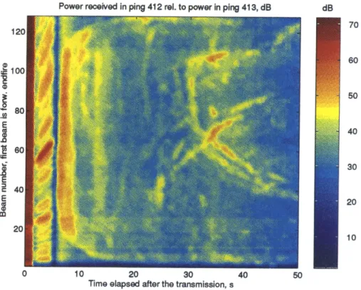
5.8 The SNR ratio against the Gaussian noise observed during ping 412. The recording of the scattering signal was made on J197 starting at 05:24 Z. Noise was recorded during ping 413 on J197 starting at 05:48 Z. Y-axis on the plot is the beam number, beam 1 is steered to the forward endfire, beam 128 is steered to the aft endfire ... 133 5.9 Average pressure level measured during 56 s observation in the

ping 413 (noise). The recording was made on J197 starting at 05:23:58 Z. High noise level in the first (forward endfire) beam is seen . . . 134 5.10 Signal measured during ping 430 in broadside beam 64 of the

Alliance receiver plotted with a solid line. The recording of the signal was made on J197 starting at 09:12:20 Z. Signal received in the same beam 20 s earlier (noise) is plotted with

5.11 The bistatic SNR ratio against the Gaussian noise observed during ping 430. The recording of the scattering signal was made on J197 starting at 09:12 Z. Noise was recorded prior to the signal arrival. Y-axis on the plot is the beam number, beam 1 being steered to the forward endfire, beam 128 steered to the aft endfire . ... 137 5.12 Direct and surface reflected paths connecting source (shown

with a star) and center of the MFA (shown with a circle). Sound speed profile used for ray calculation is shown in the left portion of the figure ... 139 5.13 Direct arrival recorded in the forward looking beam of the

Cory Chouest MFA (upper plot) and in the desensitized hy-drophone (lower plot) on the J197. Solid line: ping 411, data starts at 05:24 Z. Dashed line: ping 412, data starts at 05:36 Z, shifted backward 12 min. Dash-dotted line: ping 414, data starts at 06:00 Z, shifted backward 36 min. . . . . 141

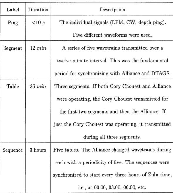
5.14 Upper plot: signal received at the Cory Chouest during ping 411. Lower plot: detected strong peaks in the received signal. Color shows received pressure level, dB re 1 aPa. X-axis is time. Early times, 5.9 to 6.6 s after the transmission, were considered. Y-axis is the beam number, where beam 1 is the forward endfire beam...145

5.15 Upper plot: signal received at the Cory Chouest during ping 412. Lower plot: detected strong peaks in the received signal. Color shows received pressure level, dB re 1 MPa. X-axis is time. Early times, 5.9 to 6.6 s after the transmission, were considered. Y-axis is the beam number, where beam 1 is the forward endfire beam...146

5.16 Angular width of individual peaks measured at the beginning of pings 411 and 412. Only strong peaks were considered. Zero values on the plot correspond to the case in which no strong peaks were detected in the time bin. Only the two strongest peaks in each cut were considered, if more then two peaks were detected. Width is in number of beams in which peaks can be seen at the -3 dB level. Linear interpolation of width was used when necessary, allowing for noninteger values of width.. 149 5.17 Separation (in number of beams) measured between the two

strongest peaks found in the time bin. Zero values are plotted for cases in which less then two strong peaks were detected. . 150

5.18 Autocorrelation function of separations between two strongest peaks detected at the time bin of data collected in the begin-ning of ping 411 (upper plot) and 412 (lower plot). Arrivals seen in the data 7 to 17 s after the transmission are considered

(early arrivals) . . . .... 152 5.19 An expanded view of the autocorrelation function of

separa-tions for early arrivals seen in ping 411 (upper plot) and 412 (lower plot) . . . 153

5.20 Upper plot: signal received at the Cory Chouest during ping 411. Lower plot: detected strong peaks in the received signal. Color shows received pressure level, dB re 1 aPa. X-axis is time. Times from 31.3 to 32 s after the transmission were considered. Y-axis is the beam number, where beam 1 is the forward endfire beam...155

5.21 Upper plot: signal received at the Cory Chouest during ping 412. Lower plot: detected strong peaks in the received signal. Color shows received pressure level, dB re 1 MPa. X-axis is time. Times from 31.3 to 32 s after the transmission were considered. Y-axis is the beam number, where beam 1 is the forward endfire beam...156

5.22 Autocorrelation function of separation between the two strongest peaks detected in the time bin of data collected at the begin-ning of ping 411 (upper plot) and 412 (lower plot). Arrivals seen in the data 35 to 45 s after the transmission are consid-ered (main lobe arrivals) ... 157

5.23 An expanded view of the autocorrelation function of separa-tion for main lobe arrivals seen in ping 411 (upper plot) and 412 (lower plot) . . .. . . .. . . . .. .. . . . .158 5.24 Comparison between signal recorded by the receiving array

and idealized beam patterns of the receiver steered into the direction where strong events were detected. The recording was made 5.859 s after the beginning of the transmission. Data were collected during ping 412 on the J197, starting at 5:36 Z. High sidelobe levels compared to the idealized case are seen throughout the entire angular range . . . 163

6.1 Signal received at the Cory Chouest. The recording was made on the J197 starting at 05:24 Z. The dotted line on the upper plot is the received signal. The solid line on the upper plot is the 1 s sliding average of the received signal (in logarithmic domain). The lower plot is the received signal with its 1 s sliding average subtracted ... 167

6.2 Histogram of the AGC scattering signal. 1 s sliding mean was removed for normalization. The recording was made dur-ing pdur-ing 411 (J197, startdur-ing at 05:24 Z), 30 to 40 s after the beginning of the transmission. The value of the normalized signal is plotted along the X-axis. Beam number is plotted along the Y-axis. Color shows the number of occurrences of the AGC signal value in each 2 dB resolution bin per 10 s of data considered ... .... ... 171 6.3 Histogram of the AGC scattering signal. 1 s sliding mean

was removed for normalization. The recording was made dur-ing pdur-ing 412 (J197, startdur-ing at 05:36 Z), 30 to 40 s after the beginning of the transmission. The value of the normalized signal is plotted along the X-axis. Beam number is plotted along the Y-axis. Color shows the number of occurrences of the AGC signal value in each 2 dB resolution bin per 10 s of data considered ... 172

6.4 Histogram of the AGC scattering signal. 1 s sliding mean was removed for normalization. The recording was made dur-ing pdur-ing 411 (J197, startdur-ing at 05:24 Z), 7 to 17 s after the beginning of the transmission. The value of the normalized signal is plotted along the X-axis. Beam number is plotted along the Y-axis. Color shows the number of occurrences of the AGC signal value in each 2 dB resolution bin per 10 s of data considered ... 173 6.5 Histogram of the AGC scattering signal. 1 s sliding mean

was removed for normalization. The recording was made dur-ing pdur-ing 412 (J197, startdur-ing at 05:36 Z), 7 to 17 s after the beginning of the transmission. The value of the normalized signal is plotted along the X-axis. Beam number is plotted along the Y-axis. Color shows the number of occurrences of the AGC signal value in each 2 dB resolution bin per 10 s of data considered .. ... ... .174

6.6 Histogram of the AGC noise. 1 s sliding mean was removed for normalization. The recording was made during ping 413 (J197, starting at 05:48 Z), 7 to 17 s after the beginning of the transmission. During this time no waveform receivable by the Cory Chouest was transmitted, therefore the reception is noise. The value of the normalized signal is plotted along the X-axis. Beam number is plotted along the Y-axis. Color shows the number of occurrences of the AGC signal value in each 2 dB resolution bin per 10 s of data considered . . . . . 175

6.7 Histogram of the average over all beams, normalized signal, measured by the Cory Chouest receiver. Solid line: Ping 411 data. Dashed line: ping 412 data. Dotted line: ping 413 (noise recording). Value of the normalized signal is plotted on the X-axis, number of occurrences in the 2 dB bin is plotted on the Y-axis. Data were collected 7 to 17 s after the beginning of the corresponding segments . . . . . 176

6.8 Histogram of the average over all beams, normalized signal, measured by the Cory Chouest receiver. Solid line: Ping 411 data. Dashed line: ping 412 data. Dotted line: ping 413 (noise recording). Value of the normalized signal is plotted on the X-axis, number of occurrences in the 2 dB bin is plotted on the Y-axis. Data were collected 30 to 40 s after the beginning of the corresponding segments . . . . . 177

6.9 Demonstration of the peak detection algorithm. Only peaks exceeding the threshold (dashed line) are selected . . . . . 180

6.10 Average separation between two adjacent peaks as a function of the beam number. Data were recorded 7 to 17 s after the beginning of the corresponding segment (early arrivals). Solid line: ping 411. Dashed line: ping 412. Dotted line: ping 413

(noise) . . . 181 6.11 Standard deviation of separation between two adjacent peaks

as a function of the beam number. Data were recorded 7 to 17 s after the beginning of the corresponding segment early arrivals). Solid line: ping 411. Dashed line: ping 412. Dotted line: ping 413 (noise) ... 182

6.12 Average separation between two adjacent peaks as a function of the beam number. Data were recorded 30 to 40 s after the beginning of the corresponding segment (main lobe arrivals). Solid line: ping 411. Dashed line: ping 412. Dotted line: ping 413 (noise) . . . 183 6.13 Standard deviation of separation between two adjacent peaks

as a function of the beam number. Data were recorded 30 to 40 s after the beginning of the corresponding segment (main lobe arrivals). Solid line: ping 411. Dashed line: ping 412. Dotted line: ping 413 (noise) ... 184 6.14 Dashed line: ratio of the average AGC signal (ping 411) to

the AGC noise (ping 413). Solid line: average separation mea-sured between adjacent strong peaks in the AGC signal (ping 411) relative to the average interpeak separation found in the AGC noise (ping 413). Signals in pings were recorded 30 to 40 s after the beginning of the transmission . . . . . 187

6.15 The average separation between adjacent strong peaks in the AGC signal as a function of time (X-axis) and beam number (Y-axis), in 1.4 s time window. The recording was made dur-ing pdur-ing 411. A relatively smaller number of peaks in each time/beam resolution bin results in higher variability of mea-sured average separation from bin to bin. Color shows sepa-ration tim e in m s...189

6.16 Standard deviation of separations between strong adjacent peaks observed in a 1.4 s window in the AGC signal as a func-tion of time (X-axis) and beam number (Y-axis). The record-ing was made durrecord-ing precord-ing 411. A relatively smaller number of peaks in each resolution bin results in higher variability from bin to bin. Color shows separation time in ms . . . 190

6.17 Solid line: average separation measured between strong adja-cent peaks as a function of bistatic angle. Dashed line: stan-dard deviation of separations. Bistatic angle 00 corresponds to the case of backscattering, 1800 is forward scattering. Upper left plot: 500 ms sliding average removed. Upper right plot: 213 ms sliding average removed. Lower plot: 107 ms sliding average removed . ... 196 6.18 Solid line: average value measured in strong peaks as a

func-tion of bistatic angle. Dashed line: standard deviafunc-tion of con-tributing values. Bistatic angle 00 corresponds to the case of backscattering, 1800 is forward scattering. Upper left plot: 500 ms sliding average removed. Upper right plot: 213 ms sliding average removed. Lower plot: 107 ms sliding average rem oved . . . 197 6.19 Number of processed peaks as a function of bistatic angle.

Bistatic angle 00 corresponds to the case of backscattering, 1800 is forward scattering. Upper left plot: 500 ms sliding average removed. Upper right plot: 213 ms sliding average removed. Lower plot: 107 ms sliding average removed . . . 198

7.1 Representation of the surface in terms of facets . . . . . 208

7.2 High resolution bathymetry data. "Valid" data selected for processing are highlighted with gray color . . . . . 217

7.3 Rms roughness measured in the individual patch of size 80 by 80 m as a function of the patch number. The average over all patches rms roughness is 6.4 m . . . . . 218

7.4 Correlation length measured in individual cuts of 80 meters length along the X axis. Average correlation length was found to be 7.3 m . . . .219 7.5 Correlation length measured in individual cuts of 80 meters

length along the Y axis. Average correlation length was found to be 7.2 m . . . .220 7.6 Estimate of power spectral density (PSD) in 80 m cuts along

the X axis. PSDs for individual patches are plotted with a dotted line. The PSD average over all patches is plotted with a solid line. The Goff-Jordan PSD is plotted as a dashed line. All PSDs are one-sided...222

7.7 Estimate of power spectral density (PSD) in 80 m cuts along Y axis. PSDs for individual patches are plotted with a dotted line. The PSD average over all patches is plotted with a solid line. The Goff-Jordan PSD is plotted as a dashed line. All PSDs are one-sided ... 223 7.8 Coordinate system for the scattering strength measurements

and modeling. The incident wave vector is in the XZ plane. The XY plane is the scattering interface. In the XY plane, the polar angle is the bistatic angle Obi, and radius is the scattering angle measured from normal (from the Z-axis) . . . . . 225

7.9 The bistatic scattering strength as a function of scattering and bistatic angle, for data in the 10 to 150 incidence grazing angle range. The polar angle is the bistatic angle, and radius is the scattering angle measured from normal (depression/elevation angle), in degrees, from 00 (at the origin) to ± 900 . . . . . . 226

7.10 The Lambert's Law prediction of the scattering strength. Macken-zie coefficient is chosen 10 log p = -15 dB. The polar angle is the bistatic angle, and radius is the scattering angle measured from normal (depression/elevation angle), in degrees, from 0'

(at the origin) to ± 900 . ... 228

7.11 Small perturbation solution for the scattering strength. Inci-dence grazing angle is 80. The polar angle is the bistatic angle, and radius is the scattering angle measured from normal (de-pression/elevation angle), in degrees, from 00 (at the origin) to ± 900 . . . 230 7.12 2-scale solution for the scattering cross section. The small

perturbation solution is used for the individual rough facet, followed by averaging over local slopes. It is assumed that the mean local slope is zero, and the standard deviation of the local slopes is 50. The polar angle is the bistatic angle, and radius is the scattering angle measured from normal (depres-sion/elevation angle), in degrees, from 00 (at the origin) to

7.13 Sensitivity of the boss solution to the value of the spectral

exponent n. Solution for n = 0 is chosen as the reference. . . .239 7.14 Boss-SP solution for the scattering strength of an individual

rough facet. Scales smaller then those accounted for by the SP theory were considered using a boss solution by Twersky. The polar angle is the bistatic angle, and radius is the scattering angle measured from normal (depression/elevation angle), in degrees, from 00 (at the origin) to + 900. . . . . . 241 7.15 Scattering strength for scattering in the plane of incidence.

The black line is the measured scattering strength. An inci-dence angle 80 was used for modeling. The blue line is Lam-bert's Law with 10 log p = -15 dB. The green line is the first order small perturbation solution for a fluid-fluid inter-face (zero shear modulus in the bottom). The red line is the 2-scale solution, where averaging over local slopes (rms angle 50) was performed. The dashed magenta line is the boss-SP solution for an individual rough facet . . . . . 243

7.16 Average incidence grazing angle in the data as a function of scattering grazing angle bin for the case of scattering in the plane of incidence . ... 244 7.17 Scattering strength for scattering in the plane of incidence.

The black line is measured scattering strength. The actual incidence angle was used for modeling. The blue line is Lam-bert's Law with 10 log t = -15 dB. The green line is the first order small perturbation solution for the fluid-fluid interface (zero shear). The red line is the 2-scale solution, where av-eraging over local slopes (rms angle 50) was performed. The dashed magenta line is the boss-SP solution for the individual rough facet . . . .. 246

A.1 Geometrical considerations for evaluating errors in estimation of the local incident grazing angle a and bistatic angle 0 at-tributed to the point in the time series . . . . . 259

Chapter 1

Introduction

1.1

Motivation

The problem of scattering of acoustic waves from rough surfaces is still exten-sively investigated. The reason for the continued attention it fairly simple. Conventionally all issues in underwater acoustics are categorized either as a direct or an inverse problem. Properties of sound scattering from rough ocean surfaces and bottoms are vital for both direct and inverse problems, i.e., in all underwater sound applications.

A direct problem usually arises in sonar engineering. The major question asked is to find the sound field incident on the receiver due to given sources

in a certain environment. The practical implication of this question is clear. Imagine for instance an arbitrary sonar system. Its performance is sought about in terms of its detection ability. Detection ability in turn is governed by the signal-to-noise ratio. It is customary to distinguish different sources of noise in the ocean. First, there is ambient noise. Second, there is system noise, i.e., noise created within the sonar system itself. At last, the ocean environment contains inhomogeneities within the water column and on its rough boundaries. The combined effect of sound scattering back from all these inhomogeneities is conventionally called reverberation. Consequently, the equivalent noise is called the reverberation noise.

As long as power radiated by the sonar is small enough, reverberation will be indistinguishable in the received signal due to the first two noise sources. This system is so-called noise-limited, i.e., noise contributing to the signal-to-noise ratio is a sum of the system noise and the ambient noise in the ocean. Neither one of those two noise sources is a function of the radiated signal itself, so sonar performance can be enhanced by increasing the power of its transmitter, thus increasing sound scattered from the target, i.e., the received signal, while leaving noise unchanged. On the contrary, power scattered from inhomogeneities will increase at the same rate as power

scattered from the targets we are trying to detect, eventually outrgrowing ambient and system noise and becoming the most important of all three noise sources. Thus powerful and capable sonar systems can become reverberation-limited. Now, to achieve better performance it is necessary to somehow control reverberation. And to make an assessment of sonar performance, a good model of the reverberation must be developed.

This emphasizes the practical importance of studying the reverberation. Also, the intrinsic property of reverberation noise as a sonar dependent prop-erty is highlighted. In contrast ambient noise is independent of the sonar, i.e., independent of the way we observe it, while reverberation noise is a function of both environment and the sonar system. Unlike any other type of noise, reverberation can not be sought independently, without considering how we observe it. Reverberation does not manifest its existence without external intervention. We encounter it while operating a sonar, or otherwise interact-ing with inhomogeneities. As in quantum mechanics, the way we observe the phenomena may alter what we see.

The inverse problem is also frequently encountered in applications, espe-cially in oceanography. In this scenario, properties of the environment are deduced from the amount of reverberation noise generated due to the

oper-ation of a certain sound source. Usually a sound source is controlled by the experimenter, however generally this does not have to be the case. Scattering of sound generated by sources already present in the ocean can also indicate the configuration of the environment.

In solving the direct problem, reverberation is usually considered as noise we would like to get rid of. Conversely, while solving the inverse problem reverberation is treated as a signal carrying information about environment. The same techniques and models are commonly used for the direct and in-verse problem solution, hence the difference between these two problems is often confined to the attitude of the researcher. Qualitative and quantitative understanding of the process of acoustic reverberation in the ocean, inher-ently interconnected with the ability to properly model the phenomenon, is vital for the solution of both the direct and inverse problems.

1.2

Objectives

To improve knowledge about rough ocean bottom scattering, a large scale experiment was initiated by ONR. The first stage of the experiment was con-ducted in 1991 employing two ships. Three ships were used in the second

stage in 1993. These stages are conventionally known as ARSRP-91 and ARSRP-93, respectively. The later one is described in detail in subsequent sections. A large volume of scattering data was acquired during the experi-ment and made available for researchers. Cited from [1], important scientific questions of the experiment were:

* What are the important mechanisms of rough, elastic, heterogeneous seafloor scattering? What seafloor features cause scattering that ap-pears event-like when high resolution signals are used? Is this scattering associated with high slope surfaces such as faults on the seafloor or fea-tures beneath a thin sediment cover? What role does propagation have to play (caustics etc.) in the generation of highly-resolved signals?

* How important is elasticity of the seafloor for scattering? Are Neu-mann, Dirichlet or impedance boundary conditions useful concepts? Are compressional and shear speed profiles necessary for accurate pre-diction? Might scattering be affected by volumetric inhomogeneities in the basement?

* Is large scale seafloor geomorphology the dominant variable in control-ling scattering? What description of seafloor geomorphology at near

wavelength scales is needed to predict scattering? Is a fractal self-similar model adequate for this small scale? What is the sensitivity of measured and model results to interface characteristics like fractal/non-fractal of, if applicable, Gaussian/non-Gaussian statistics and within divisions, what is the sensitivity to variation of parameters like the five in the Goff-Jordan model?

* What is a good characterization of seafloor scattering? Can the prop-erties of the reverberation be described using stochastic concepts, or is a more deterministic approach necessary? If a stochastic approach can be used, is the concept of scattering strength as used in the sonar equa-tion useful for quantifying scattering with a high resoluequa-tion system? Do simple models like Lambert's Law have a useful role in describing the scattering?

In the following I will analyze and model the midfrequency data (A = 6m),

1.3

Major results

Analyzing the data I found that the received scattering signal is a highly nonstationary function of time. I show that two goals are achieved by re-moving local short-time average from the received signal. First, this proce-dure allows one to separate the signal into its "slow" and "fast" components, where the slow component (local mean) carries information about the first order statistical properties of the signal, and higher order statistical prop-erties are encapsulated in the fast component (signal with its local mean removed). Second, the resulting fast component is a stationary stochastic process, which simplifies its statistical analysis. Subsequently, I show that different physical parameters control first and higher order statistical prop-erties of the received signal, hence slow and fast components can be analyzed and modeled independently.

Considering the higher order statistical properties of the received signal, I find that discreteness of the scattering process results in a slight deviation of the received signal probability density distribution away from the Gaussian at high levels of the received signal. However, a substantial difference be-tween signal and Gaussian noise is found considering temporal distribution of individual features in the received signal (peaks). Therefore, I conclude

that analysis of individual peaks in the received data is a better indicator of statistical properties of the received signal, and hence a better reflection of the physics of scattering. Additionally, I find that the major contribution to scattering is generated by the O(A) scales on the bottom, which supports a separation of scales hypothesis [2, 3], and emphasizes the importance of wave effects. Later I show that the first order statistical properties of the received signal (related to the scattering strength) are controlled by the experimental geometry and large scale geomorphology, with essential roughness scales on the order of the sonar footprint size L0 I 100 + 1000 m.

Then it becomes clear that the scattering observed during the ARSRP-93 experiment is a multiscale process, and therefore a multiscale wave scat-tering theory is required for its proper understanding and modeling. This explains the apparent mismatch between the experimental data and the geo-metric Lambert's Law [4] which assumes infinitely small incident wavelength. Small perturbation theory [5, 6] accounts for the finiteness of the incident wavelength and captures the correct functional dependence of the scattering signal, however underpredicts its level by about 10 dB in the back directions. Using the separation of scale hypothesis I suggest that small features not accounted for by the first order small perturbation (SP) solution are

responsi-ble for the enhanced scattering in the back directions. To improve the model, I propose a composite boss - SP theory. Within this model, the solution is sought of as an incoherent superposition of contributions from small scales, accounted via the boss theory, and the SP solution. Conceptually this model is in line with the standard 2-scale theory [7], where the solution for a rela-tively large scattering patch is sought as a combination of SP and Kirchhoff solutions. Finally, I show that the model developed results in an improved fit with the experimental data (to within 3 dB).

1.4

Notation

I use complex representation of the acoustic field parameters throughout, harmonic time dependence is implied unless otherwise stated. Consequently the physical value of a parameter is given by the real part of its complex representation. So, for instance, if stands for the complex amplitude of the parameter (, the value of the parameter observed in an experiment is

1

physical = Rc = + *), (1.1)

2

where superscript star as usual means complex conjugate.

Overbar is chosen to designate time average of a random function. Often 39

a square value of the complex amplitude of a harmonic function averaged over its period is of interest. In complex notation it becomes

2 (1.2)

hence, for a physical (observable) value

1hysical

2 2 . (1.3)

As a shortcut for the mean square value of a complex amplitude, the over-bar is omitted, so for a harmonic function (2 stands for (2 unless otherwise stated.

Angle brackets () are chosen to indicate an ensemble average of a random function. An average over the period and the ensemble mean square value of the complex amplitude can be expressed as M) or equivalently in the

shortcut notation as ( 2).

1.5

Thesis organization

First, in Chapter 2 I present a brief outline of the problem. I start the dis-cussion with a review of the basics of sound propagation in the ocean. This naturally leads to the recapitulation of classical scattering terminology. It

then becomes clear that an adequate model of rough surface scattering is a cornerstone in understanding reverberation phenomena and, consequently, reverberation noise. In Chapter 3 rough surfaces are described in terms useful for the subsequent development of the scattering theory used in this thesis. Chapter 4 briefly presents several classical rough surface scattering theories. In Chapter 5 the ARSRP experiment is described. This experiment was de-signed to refine our knowledge of low grazing angle reverberation. Analysis of higher order statistics in the time series acquired during the ARSRP ex-periment is presented in the Chapter 6. Subsequently in Chapter 7 I analyze the bistatic scattering strength observed during the ARSRP experiment. Fi-nally, in the Chapter 8 I present a summary of the thesis and suggestions for future work.

Chapter 2

Problem Outline

A standard sonar experiment is designed as follows. A signal consisting of a sound pulse is radiated from a source. The signal propagates to the receiver in the inhomogeneous ocean environment. Knowing the source and the envi-ronmental parameters, one would like to compute the signal registered by the receiver. Several issues should be confronted in order to resolve the matter.

* First, a mixture of the signal with ambient noise is inevitably recorded. Hence, proper understanding and adequate modeling of the noise in the ocean is essential to detecting and studying scattering and rever-beration.

* Second, a way must be found to determine the paths followed by the 42

sound signals, and to decide how sound parameters might have been changing along these paths. This means that a model of sound propa-gation in the environment has to be established.

* Third, inhomogeneities are present in the path of the sound waves, hence there will be an interaction between sound and inhomogeneities, or in other words scattering of the incident sound wave from inhomo-geneities. The properties of the sound wave can be dramatically altered during this interaction, hence the importance of studying scattering.

Traditionally three classes of scattering are distinguished. The first class consists of scattering from individual inhomogeneities that can be distin-guished in the received signal. In turn, such an inhomogeneity is referred to as a "target" or "scatterer". Often the observer attitude alone dictates the choice between target and scatterer, so that any unwanted target might be called a scatterer.

The second class may be described as follows. When scattering from many inhomogeneities, somehow distributed in the entire volume of the wa-ter, contribute to the received signal, the interaction of the acoustic field with these inhomogeneities is usually designated as volumetric scattering. Usually these inhomogeneities are considered small and abundant, so that individual

scatterers are not seen, and the received signal is some sort of aggregation of individual contributions.

The third class is scattering from a surface. This type of scattering is encountered when the inhomogeneities are two-dimensional, or are a distri-bution of three-dimensional inhomogeneities on the interface. Usually within this class of scattering problems, scattering from rough surfaces is distinct from scattering from smooth surfaces, thus forming a lower level of catego-rization.

Sometimes, the combined effect of scattering from all inhomogeneities presented in the environment is called reverberation [8]. However, often re-verberation has a more restrictive meaning, so that only scattering from the ocean surface, bottom and volume into one direction only (back to the source of the signal) is termed reverberation [9]. Sometimes the subdivision between different kinds of scattering, and between scattering and reverberation, ap-pears artificial. For instance, reverberation clearly is not an independent phenomenon and can be understood through its components: propagation and scattering. However, the delineated classification often proves effective in distinguishing between different natural phenomena, and so will be followed.

To develop a proper understanding of the sonar experiment, all three problems outlined must be resolved. In this thesis I will mostly concentrate on scattering issues. However, results of the sonar experiment (ARSRP) will be used to enhance our knowledge about the rough bottom scattering. Hence, to build a basis for the interpretation of experimental results, I start here with a brief outline of how the first two problems (noise and propagation) can be approached, followed by the essential scattering terminology.

2.1

Ambient noise in the ocean

More complete discussion of ambient noise can be found in [4, 10, 11, 12]. A brief outline of the terminology follows.

Ambient noise is "the sound of the ocean" [10], i.e., that part of the acoustic field that exists in the ocean without any intervention from the researcher. Ambient noise constantly varies with time and location. Knowing its exact level at each moment is hardly possible, so stochastic models of noise in the ocean environment are pursued.

Mean square noise pressure p2 detected by an omnidirectional receiver is a common measure of ambient noise energy. To indicate frequency

depen-dence and directivity of the noise power, the spectral power density of noise

Wn(w, k) is introduced, where a Fourier transform is performed over both

temporal and spatial variables, k is the wave vector associated with the noise and w is the noise frequency. This quantity normally is used as a measure of the noise field. Mean square pressure p2 is simply related to the power spectral density:

P =

J

dw

W

(w, k)dk.

(2.1)

The input power of the unwanted interference measured by the system with transfer function TF(wk) is proportional to the actual mean square

pressure of noise p2, ,act

Pn,act = dw

J

-OO -OO0

This number can serve as an indicator of the actual noise limiting the sonar

performance. However, in practice usually its base ten logarithm, called noise

level, is used instead:

2.2

Sound propagation in the inhomogeneous

environment

The science of sound propagation modeling is still growing nowadays. Several wave theories have been recently developed in addition to existing ones [13,

14, 15, 16, 17, 18, 19, 20].

The reason for continuous attention to this topic is that the ocean is an extremely complicated environment, where all parameters are constantly changing with depth, range and time. Due to the presence of boundaries (ocean surface and bottom, targets) several different paths connecting source and receiver are generally possible. This multipathing adds complexity to an already complicated problem.

Ray theory (which I will limit myself to) was the first to appear, as an extension of classical geometrical optics. Although a tremendous amount has been accomplished in pursuit of wave theories of sound propagation, rays are still a powerful tool for understanding and modeling [21, 10, 22, 23, 24].

Rays carry an intuitive meaning, and often can provide useful physical insights into the nature of sound propagation. Ray solutions require the least mathematical investment, and frequently can be performed analytically. And

surprisingly enough, a properly executed ray solution often has the same level of quantitative precision as more involved wave theories do. I use rays in the analysis of the ARSRP experiment, hence a summary of the theory is briefly outlined here.

A ray is an imaginary line drawn in the direction locally normal to the wavefront. The computation of this line is referred to as ray tracing. Rays outline the direction of the field propagation, i.e., they are a geometrical property of the field. Additional considerations allow one to determine how energy associated with the field changes along the ray. To derive ray equa-tions one often starts with a linear sound wave equation [22, 9]:

1 a2(

2 = (2.4)

c2 M

t2'

where r is the coordinate vector in the three dimensional space, c(i) is the sound speed in the ocean, t is time, and 1 is the scalar acoustic potential. All physical parameters of sound can be expressed in terms of the potential. For instance, particle displacement d, velocity ', sound pressure p and energy flux F take the following form:

O 92 (D a2 4D I:

d= V( , = -V , P=-P- F - (25)

where p is the density. Then solution to the wave equation is sought in 48

the form of a harmonic wave: o = (o( • e- iw(t-r(-)), where 7 is called the

eikonal. Ray approximations are valid when both Go(r) and VT(r) are slow functions of F, so that the following is correct:

,0

2 _{7VT 0 U} 2 _U2

<< 2 2 2 « 2 (2.6)

Go c Io cc

Then the wave equation is reduced to the well known eikonal equation:

1

V2T 2.(2.7)

Approximating the solution as a locally plane wave, one ends up with 1

,7r = -, (2.8)

C

where n is the local normal to the wave front. Ray tracing equations subse-quently obtained for the case of in-plane propagation in the (xz) plane take the form:

d (I COS 0)=

I

_(cos)

-

_(2.9)

-sin 0) = 1 ac

dt c C az'

where 0 is the grazing angle measured from horizontal.

Finally, for the range independent environment (2.9) can be further re-duced to the differential Snell's law:

cos 0_{C = a}

= const, _(2.10)

where the horizontal slowness a acts as the ray label.

The ray solution gives only the direction of energy propagation. However it exposes an important property of rays. Substituting the solution in the form of the plane wave into (2.5) one can see that F = pWID2kin, hence energy flow is parallel to the ray direction.

Consider now a tube of rays. Conservation of energy requires that energy flow through any tube cross section is constant. Then the equation for the sound energy change along the ray is:

p2 = p p1c2A, _P2cjA2 (2.11)

where P ,2 are mean square pressure amplitudes, P1,2 are densities and c1,2 are

sound speeds observed in cross sections 1 and 2 with areas A1,2, respectively. Generally, equations (2.10) and (2.11) are solved numerically for any given sound speed profile c(z). However, for several profiles there are analytical solutions. For instance, if the sound speed is a linear function of depth, i.e.,

c(z) = c(zo) + g(z - z0), then the ray path is a circle with radius of curvature

given by

r = -1/ag. (2.12)

Usually the sound speed profile is known through direct or indirect mea-surement at several depths. Then these meamea-surements can be approximated

with a piecewise linear curve. Each piece with a constant gradient g of the sound speed define a layer. In each layer ray calculations can be carried out analytically resulting in the following expressions for sound propagation forward from a point source [10]:

R12 = .(sin 01 - sin 82), Z12= (cos

92

where R12 and Z12 are horizontal and vertical distances traveled by the ray, 91

and 92 are grazing angles at the entrance and exit from the layer, respectively, determined via Snell's law, t12 is the travel time, and W is the power radiated

by the source. Using the forms of (2.13) in each layer results in an efficient numerical solution for the sound pressure.

The first three equations in the (2.13) are an outcome of the ray tracing equations (2.9), hence valid when (2.6) is true. For a plane wave propagating in the layered medium with sound speed c(z) having gradient g(z) dependent on the vertical coordinate z only it is equivalent to [9]:

ld

1 d log kz << 1. _(2.14)

kz dz

For steep rays with kz = O(k) it can be further reduced to gA/c << 1 51

[9], which sometimes is said to be the ray theory applicability condition. But in the vicinity of a turning point k, -+ 0 and condition (2.14) become inapplicable for an arbitrary small g. However, it was shown to primarily affect the phase accumulated along the ray path and the field amplitude calculation, and to have less profound effect on the ray direction calculation [9, 25]. The last equation in the (2.13) is a result of the energy conservation consideration along the ray tube. Near the caustic the ray tube diameter shrinks to zero. It results in an infinite value of the field amplitude, from use of the last equation of (2.13). More precise WKB approximations [9, 25] or more involved methods of the ray tube calculation [22] can in fact overcome this difficulty. Then caustics can be safely included into the ray theory applicability domain. Matched asymptotic expansion can be used to treat turning points correctly [25]. However, all this results in somewhat different and more complicated ray tracing equations. Using simplified forms (2.13) specifically restricts one to the regions away from caustics and turning points.

2.3

Basic scattering terminology

A ray can be an adequate tool for sound propagation modeling when inho-mogeneities are smooth, i.e., when medium parameters are changing only slightly on the scale of the wavelength. Hence ray theory can not be used near rough boundaries. Examination of wave propagation theories indicate the same tendency: the presence of a boundary in the domain of the solu-tion can not be handled. Approximasolu-tions made to enhance performance of the theory in application to propagation preclude its use in the vicinity of boundaries. A specific tool is required to properly address the issue, i.e., a scattering theory. Then propagation theory can be used to trace the sound to and from the interface, and scattering theory then describes the interaction with the boundary.

Boundaries in the ocean are represented by the bottom and surface, by coast lines, and also by wanted and unwanted targets that may exist within the water column. In the next subsections essential terminology is briefly summarized.

Considering scattering it is advantageous to make use of the following two assumptions. First, it is known that sound waves decay exponentially as they propagate due to absorption. By no means can we neglect absorption in

propagation. However only rarely does absorption affect scattering, hence it will be ignored from now on. The other limitation reasonable to presuppose is local homogeneity and isotropy of the medium in the vicinity of the target or scatterer. These two restrictions allow one to effectively isolate scattering effects from those imposed by propagation.

2.3.1

Scattering from targets: target strength

Consider a plane sound wave with pressure amplitude Pi, wave vector k and wavelength Ai = 27r/ki incident upon a body. In scattering this body is

often referred to as a target. Incident acoustic pressure causes vibrations on the surface of the target and within its volume, and a new system of waves originates from these vibrations. This part of the acoustic field is called the scattered field or equivalently the scattered wave.

Generally the scattered pressure field in the vicinity of the target is quite complicated. However, at large distances from the target with characteristic size D defined by r >> D2_{/A , the scattered field can be represented as a} locally plane spherically spreading wave traveling out from the target to the observer. Thus, a target at large distances behaves as an effective directive source of the scattered wave. This is the so-called far field approximation.

The pressure p, generated by this source can be expressed as [26]:

p.( = f f ,, z) -I( , (2.15)

r

where the scattering amplitude f incorporates both the amplitude and phase of the scattered wave in the far field in the direction k, when the target is illuminated by a plane wave propagating in the direction ki. Therefore the scattering amplitude f is a complete description of the scattering process when distance from the region where scattering takes place is large enough. Equation (2.15) is a definition of the scattering amplitude

f.

It is customary to introduce several more measures of scattering called "cross sections" and "target strength". Even though descriptions in terms of a cross section or a target strength is incomplete, it is often convenient and traditionally used.

First, for targets of finite extent it is appropriate to define a geometric cross section ag which is equal to the normal projection of the area of the target on the direction of incident wave propagation.

equivalent source level of the scattered wave [26, 27]:

VV8(kj)

as(i) = lim (2.16)

r- oo

I

where 1i is the incident wave intensity, and W, is the total power scattered, averaged in time, due to a plane wave incident from direction ki. Imagine the scattering process as an energy transfer from the incident to the scattered wave. Then the scattered power W, is equal to the power carried by the incident wave in the absence of the target through its scattering cross section area as. Hence, scattering cross section conveniently measures the effective geometrical cross section of the target as seen by the incident wave.

With a, so defined, the scattered mean square pressure at large distances from the target can be expressed as

2 a2 ki) B 2sk i)

2 = p2 ( , (2.17)

PS 4irr2 dt(k₂)

where Bt (ks, ki) is a squared beam pattern of the effective scattering source, and directivity factor dt(ki) = 1/4w.

f

pattern averaged over the entire angular space. Clearly, both values of the beam pattern and scattering cross section are required to describe the scat-tering. A convenient way to merge these two terms into one is to introduce

the differential scattering cross section:

ad(ks, fi) = lim (2.18)

r-+oo I

where Is is the scattered wave intensity observed at range r in the direction

ks due to the plane wave propagating in the direction ki. Consequently, the

scattered pressure at large distances from the target is given by:

2 P2 ad (ks) k%)r)

ps k2r, r2 (2.19)

Frequently in applications, bistatic scattering cross section and backscat-tering cross section are used along with the differential scatbackscat-tering cross

sec-tion:

In

Ub (k,

ki)

= 47ro-d(ks,

I ),

_(2.20)

9b(ki,) = 47rd(-k, ki).

Except for a scaling factor, bistatic and differential scattering cross sections can be used interchangeably. Backscattering cross section has a much more restricted meaning since only one direction is considered.

The other way of target description is found through its target strength defined as follows:

-.. g r2 . p2(k -I'k i

,r

T(ks, ki) = 10 log lim 2 dB re rf, (2.21)

where usually the reference distance rref = lm. Sometimes the target strength definition is restricted to backscattering only. Since I am gener-ally interested in scattering into all directions, I shall use (2.21) as the target strength definition. Target strength so defined can be easily related to scat-tering cross sections, e.g.:

Ud(ks, ki)

T(k, i) = 10 log r2'f dB re rre. (2.22)

ref

Appropriate modification of (2.19) result in the following expression for sound pressure level in the scattered signal:

-. -,p2 - r2

Lp(ks , r) = 10 log ' z+ T(ks, ki) - 10 log 2,f dB re rref&Pref, (2.23)

Pref ref

where the usual definition of the sound pressure level is used:

2

LP= 10log 2 , dBrepref, (2.24)

Pref

where in underwater acoustics prefy = 1pPa.

Historically notation of target strength is preferred in acoustics, and scat-tering cross section is a conventional choice in electromagnetics. There is no reason beyond tradition to favor target strength, differential or bistatic cross section as a scattering descriptor.

Although all methods of target characterizations outlined here are fre-quently used interchangeably, only scattering amplitude is a complete