Bayesian network models of biological signaling pathways

(1)

Bayesian network models of biological signaling

pathways

by

Karen Sachs

Submitted to the Department of Biological Engineering

in partial fulfillment of the requirements for the degree of

Doctor of Philosophy in Biological Engineering

at the

MASSACHUSETTS INSTITUTE OF TECHNOLOGY

@ Massachusetts

July 2006

Institute of Technology 2006. All rights reserved.

Author ... ,

.

... ...

.

Department of Biological Engineering

July 13, 2006

-~ A

Certified by

... t " .

...

..

i.

bur

Douglas I

nbeurger

Whitaker Professor of Biological Engineering, Chemical Engineering,

and Biology; Director, Biological Engineering Division

A

hesis Supervisor

/ /

;

1 Accepted by...

. .

.

...

....

.dzn

MASS AC T .- - -1S O f 1 .- - -MASSACHUSETTS IN OF TECHNOLOGY

NOV 1:5 2006

LIBRARIES

arman, epartment ommttee on ra u tudents

(2)

Thesis Committee

Approved by ... ...

Bruce Tidor Professor of Biological Engineering Professor of Computer Science Chair of Thesis Committee Approved by ...

Douglas A. Lauffenburger Whitaker Professor of Biological Engineering

Professor of Chemical Engineering Professor of Biology Thesis Supervisor Approved by ...

Christopher B. Burge Professor of Biology Thesis Committee Member Approved by ...

Peter K. Sorger Professor of Biology Thesis Committee Member Approved by ...

Steven R. Tannenbaum Professor of Biological Engineering Thesis Committee Member

(3)

Bayesian network models of biological signaling pathways

by

Karen Sachs

Submitted to the Department of Biological Engineering on July 13, 2006, in partial fulfillment of the

requirements for the degree of

Doctor of Philosophy in Biological Engineering

Abstract

Cells communicate with other cells, and process cues from their environment, via signaling pathways, in which extracellular cues trigger a cascade of information flow, causing signaling molecules to become chemically, physically or locationally modified, gain new functional capabilities, and affect subsequent molecules in the cascade, cul-minating in a phenotypic cellular response. Mapping the influence connections among biomolecules in a signaling cascade aids in understanding of the underlying biological process and in development of therapeutics for diseases involving aberrant pathways, such as cancer and autoimmune disease. In this thesis, we present an approach for automatically reverse-engineering the structure of a signaling pathway, from high-throughput data. We apply Bayesian network structure inference to signaling protein measurements performed in thousands of single cells, using a machine called a flow cytometer. Our de novo _{reconstruction of a T-cell signaling map was highly accurate,}

closely reproducing the known pathway structure, and accurately predicted novel pathway connections. The flow cytometry measurements include specific perturba-tions of signaling molecules, aiding in a causal interpretation of the Bayesian network graph structure. However, this machine can measure only -4-12 molecules per cell, too few for effective coverage of a signaling pathway. To address this problem, we employ a number of biologically motivated assumptions to extend our technique to scale up from the number of molecules measured to larger models, using measure-ments of overlapping variable subsets. We demonstrate this approach by scaling up to a model of 11 variables, using -15 overlapping 4-variable measurements.

Thesis Supervisor: Douglas A. Lauffenburger

Title: Whitaker Professor of Biological Engineering, Chemical Engineering, and Biology; Director, Biological Engineering Division

(4)

(5)

Acknowledgments

I have often thought, that if I ever did finish my thesis, I would have many people to thank.

To my advisor, Doug Lauffenburger, thank you for being my mentor during my time at MIT. I am really grateful that you were willing to take a chance and give me the opportunity to follow my interests (even though it may have seemed somewhat risky). I have always appreciated your confidence in my ability to figure out this project, even (perhaps especially) when I was not so sure of this myself. I want to thank you for your persistent patience and support, which have been tremendously helpful (and inspiring), and have defined a standard for me which I will try to emulate when I supervise students. I hope that I am lucky enough in my future work to find others with your enthusiasm, brilliance, and appreciation of the intricacies of systems biology. They will have a hard act to follow.

To my thesis committee, thank you for being always focused and engaged when pondering my project. I have been fortunate to receive guidance, feedback and sugges-tions which have challenged me to think about my project from different perspectives, and I feel that I am a better scientist due to my interaction with my committee over the years.

To Bruce Tidor, head of my committee, thank you for being tolerant of summer-scheduling, for sticking with me till the end, and for many challenging discussions. Your perspective, as one doing related but not immediately similar work, has been very valuable. To Chris Burge, thank you for being willing to fill in at a late stage, and thank you for your thoughtful feedback and specific suggestions, particularly regarding CPD visualization. To Steve Tannenbaum, I want to thank you for making me feel so welcome when I first arrived at MIT, for being the first to make BE (then BEH!) seem like a home, and for all your help, especially while I was still looking for

a lab. I have not forgotten your concern for my welfare, I have always appreciated

it and have always been glad to see you, in committee meetings or just around MIT.

(6)

insight not only in my committee meetings but also in my many interactions with you throughout the years, through BIM/CDP related meetings. Finally, to David Gifford, thank you for adopting me into your group, for always going out of your way to make me feel welcome at group events, meetings and retreats, and for many useful suggestions during my thesis work. The affiliation with you and your group has been an invaluable resource for me in all my years here.

I had the incredible fortune to obtain an additional mentor for my thesis project. I stumbled across Dana Pe'er at a conference in St. Louis, and we soon developed a wonderful collaboration. Dana and I spent many pleasant hours at Peets coffee, discussing, among other things, Bayesian networks and their applications to signaling pathways. Thank you for so many stimulating conversations, for teaching me and looking out for me, and for investing your energy, enthusiasm and brilliance into my project. Myself and my project benefited tremendously from your contributions.

To members of the Lauffenburger and Griffith groups, and members of CDP, the interaction with you all has helped to make MIT a place of amazing intellectual energy and excitement. It has also made doing science a fun and stimulating expe-rience. I want to thank former Lauffenburger lab members, including Kirsty Smith, Bart Hendriks, Stas Shvartsman, Dan Kamei, Lilly Koo, Keith Duggar, Ann Dewitt and Casim Sarkar for a supportive lab environment early on, and Peter Woolf for illuminating discussions on Bayesian networks and numerous other topics. To CDP members and more recent lab members, particularly Birgit Schoeberl, Lucia Wille, Sampsa Hautaniemi, Suzzane Gaudet, John Albeck, Bree Aldridge, Kevin Janes, Melissa Kemp, Megan Palmer, John Burke and Pam Kreeger, I feel like this group has been an integral part of my thesis project. Thank you for the wonderfully open, collaborative and friendly environment, and for countless useful discussions. Finally, to JoAnn Sorrento, thank you for your friendly attitude, patience, and willingness to help with everything from room reservations to gardening.

To members of the Gifford group, past and present, thank you for many techni-cal explanations, advice with coding, useful discussions, and help with the specifics of the likes of unix and LaTex. Special thanks to Alex Hartemink, for getting me

(7)

started with Bayesian networks via many discussions and patient explanations. To Alex Phillip Rolfe, Matt Rasmusen and Ken Takusagawa, thank you for millions of snippets of invaluable technical advice (especially Alex, who has been around more and therefore has answered more questions); to Georg Gerber for many helpful dis-cussions and generally supportive attitude; to Tim Danford for disdis-cussions on many topics including graphical models and coding principles; to Yuan (Alan) Qi for your willingness to answer difficult Bayes nets questions; to Robin Dowell for your per-sistent warmth and advice on post doc issues, and to Kenzie MacIsaac for being an overall marvelous officemate. Last but not least, to Jeanne Darling, thank you for fixing a thousand problems for me over the last several years, and for being an inspir-ing person. To all of you, thank you for sharinspir-ing your (seeminspir-ingly infinite) expertise and providing a friendly environment in the group.

To other members of the community, who taught me much and enriched my experience at MIT: Tommi Jaakkola, Ernest Fraenkel, Joachim Theilhaber, James Sherley, Bevin Engelward and John Essigman. Also thanks to Teresa Wright, who introduced me to BE and helped me get started in the department, and to Rohit Singh, for lending me his expertise on several occasions.

To my fabulous friends and classmates, Hiroko Sudo, Yelena Margolin, Helen Banava, Sam Boutin, Maya Said, thank you for being friendly, fun and supportive. To the people who were so important to me in (and since) my early years at MIT: Heelo Sudo. Chrissy Guth, Nati Srebro, Thandi Muno, Maxim Kalashnikov; to the people who arrived slightly later: Alexandria Sams, Jenn Cheng, Tanyel Kiziltepe, Peter Bermel, Claire Monteleoni, Ulrike Spaete, Martin Zalesak; to the people who (unfortunately) I only met in my last year or so: Leah Henderson, Patrick van der Wel, Tammy Shoham, Solomon Itani, Hariharan Rahul, Jennifer Carlisle, Gregory Marton; and to those who I have known for ages: Masha Ishutkina, Misha Davidson, Irit Orgil, Vered Greenberg: thank you for the hikes, the talks, the coffee breaks, dinners, bike rides, hours at the gym, trips to the Walden, thanks for help with research, for help with life, for giving me perspective when I needed it and for being incredible friends. My time at MIT has been wonderful because of all of you; along

(8)

the thesis process, finding people like you is the greatest accomplishment. (I have much more to say, but I had better stop here, for fear of having a 400-page thesis)

Finally, to my family, your boundless love and support has always been my foun-dation in everything I do. Thank you to my parents, who solved physics problems for me and explained imaginary numbers at the first hint of curiosity. To my father, Rimmon Sachs, thank you for your infinite dedication, and for investing hours in solving math problems and deciphering buggy code whenever I needed help. To my loving mother, Ella Sachs, for being thrilled at everything I do and am. To my sister Carrie, for always reminding me that she is proud of me and always being eager for my success. To my sister Zohar, for guiding me along the grad school process and helping me, as always, in countless ways. Grad school was a million times better because you were there. To my brother Shai for your calm, supportive ways, for always thinking about others, and for helping me with coursework. To my littlest sister Noga, thank you for the very real help you provided on several occasions and for your willingness to do so, thank you for always encouraging me when I was down, and thanks for being a wonderful and supportive sister. And to my nephew Adam, thank you just for being your adorable self.

(9)

List of Figures

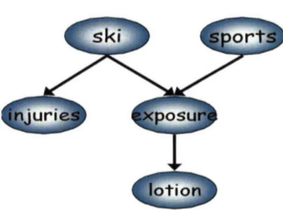
2-1 A Bayesian network depicting statistical dependencies among variables. The variables injury and lotion are statistically

depen-dent upon the variable ski ... 45

2-2 The Bayesian network including additional variables. Ski and sports together predict sun exposure, which is a good predictor of

lotion use. . . . .. 46

2-3 A Bayesian network structure for the variables pollen, allergy, cold

and sneezing ... ... 48

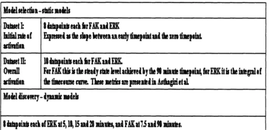
3-1 Data summary. For model selection, data sets I and II are used to score static models. Data set I is the initial rate of activation from Asthagiri et al, 1999; data set II is overall activation. Model discovery examines dynamic models and therefore employs the unprocessed time

course data. ... 79

3-2 Candidate and control models. "Cue" represents the signal from the interaction betwen fn and integrin, F is FAK, and E is ERK2. MO is the control model. An additional model identical to M4, but with the edge from F to E reversed, is not represented because it is in the same equivalence class as M4 and will, therefore, always score the same. 81

(14)

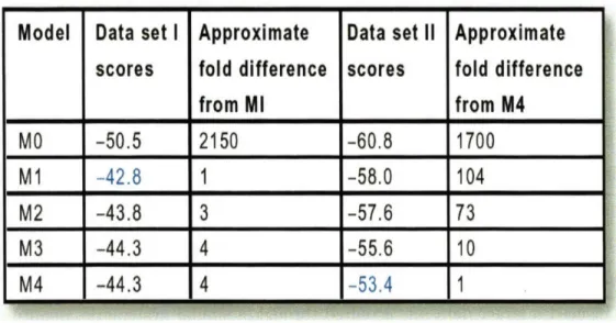
3-3 Model scores. Data set I is initial rate of activation from Asthagiri et al; data set II is overall activation. Columns 3 and 5 indicate to what degree the top-scoring model explains the data better than the indicated model. This fold difference is equal to e to the power of (difference in model scores). ... . 82

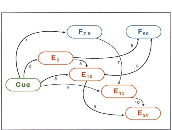
3-4 Features common to high-scoring graphs. The model presented com-prises a weighted average of high-scoring graphs from 200 runs of the search algorithm. "Cue" represents the signal from fn and integrin, E is ERK2, and F is FAK. Subscripts indicate time in minutes. Light arrows are features with a posterior probability of 0.5 to 0.85; dark ar-rows represent consensus arcs or arcs with posterior probability 0.85. Arcs 1 through 10 are numbered for convenience. .. . ... 84

3-5 Diagram of TNF-induced signaling. Molecules either measured or ma-nipulated in this study are shown in green. Figure source: Suzzane

Gaudet, Kevin Janes ... 87

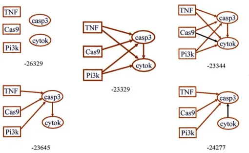
3-6 Proposed models and their scores. The scores as reported as the nat-ural log of the relative probabilities. Therefore, the difference in score

between models is expS coreMi- s coreMj (i.e. e to the power of (Difference

in score between the two models)). The correct model scores higher than the others by a factor of at least 1000 ... . ... 88

(15)

4-1 Bayesian Network Modeling with Single Cell Data A. Schematic

of ]Bayesian network inference using multidimensional flow cytometry data. Nine different perturbation conditions were applied to sets of individual cells (see Table 1A). A multiparameter flow cytometer si-multaneously recorded levels of 11 phospho-proteins and phospholipids in individual cells in each perturbation dataset (see Table 1B). This data conglomerate was subjected to Bayesian network analysis, which extracts an influence diagram reflecting dependencies and causal rela-tionships in the underlying signaling network. B. Bayesian networks for hypothetical proteins X, Y, Z, and W. (a): In this model X influ-ences Y which, in turn, influinflu-ences both Z and W. (b): Same network except Y was not measured in the dataset. C. Simulated data that could reconstruct the influence connections in Figure 4-1, B (this is a simplified demonstration of how Bayesian networks operate). Each dot in the scatter plots represents the amount of two phosphorylated pro-teins in an individual cell. (a) Scatter plot of simulated measurements of phosphorylated X and Y show correlation. (b) Interventional data determine directionality of influence. X and Y are correlated under no manipulation (blue dots). Inhibition of X affects Y (yellow dots); inhibition of Y does not affect X (red dots). Together this indicates that X is consistent with being an upstream parent node. (c) Simu-lated measurements of Y and Z. (d) A noisy but distinct correlation is observed between simulated measurements of X and Z. ... . 92

(16)

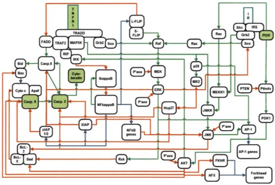
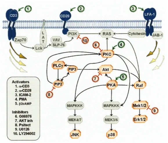
4-2 Classic Signaling Network and Points of Intervention. Graphical illus-tration of the conventionally accepted signaling molecule interactions, the events measured, and the points of intervention by small molecule inhibitors. Signaling nodes in color were measured directly. Signaling nodes in gray were not measured but are presented to place the signal-ing nodes that were measured within the context of contextual cellular pathways. Interventions classified as activators are color-coded green and inhibitors are color-coded red. Intervention site of action is indi-cated in the Figure. Arcs are used to illustrate connections between signaling molecules; in some cases the connections may be indirect and may involve specific phosphorylation sites of the signaling molecules (see Figure 4-7 for details of these connections). Note that this figure contains a synopsis of signaling in mammalian cells and is not repre-sentative of all cell types, with inositol signaling co-relationships being

particularly complex. ... 93

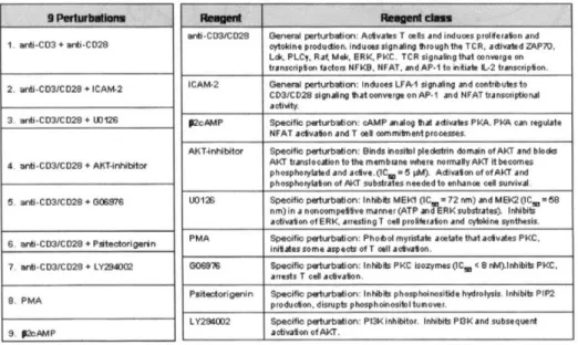
4-3 Conditions used and biological effect. Left hand column outlines

the conditions used in this study. Middle column lists the specific reagents used in each perturbation condition and the right hand column classifies the reagent class into either a general perturbation that overall stimulated the cell or a specific perturbation that acts on a defined set of m olecules .. . . . . 94 4-4 Example scatterplots of the multicolor flow cytometry data used. Each

dot in the scatter plots represents the amount of two phosphorylated proteins in an individual cell. A. Scatterplot of phosphorylated proteins Raf and Mek shows a clear correlation, similar to the simulated data presented in Figure 4-1, panel a. B. Scatterplot of PKC and PKA displays a far noisier dependency that is not apparent by eye. The data used contains the entire range between the two examples in this figure. Given sufficient data, the Bayesian network is able to overcome the noise and extract these relationships. . ... . . 95

(17)

4-5 Molecules measured and antibody specificity. In the left hand col-umn are shown target molecules measured in this study. These were assayed using mAb to the target residues (site of phosphorylation or phosphorylated product as described). ... . 96

4-6 Bayesian Network Inference Results. A. Network inferred from flow cy-tometry data represents expected outcomes. This network represents a model average from 500 high-scoring results. High-confidence arcs, appearing in at least 85molecules are used to represent the measured phosphorylation sites, (See Figure 4-5). B. Inferred network demon-strates several features of Bayesian networks. (a) Arcs in the network may correspond to direct events or, (b) indirect influences. (c) When intermediate molecules are measured in the dataset, indirect influences rarely appear as an additional arc. No additional arc is added between Raf and Erk because the dependence between Raf and Erk is dismissed by the connection between Raf and Mek, and between Mek and Erk (for instance, see Figure 4-1). (d) Connections in the model contain phosphorylation site-specificity information. Since Raf phosphoryla-tion on S497 and S499 was not measured in our dataset, the connec-tion between PKC and the measured Raf phosphorylaconnec-tion site (S259) is indirect, likely proceeding via Ras. The connection between PKC

and the undetected Raf phosphorylation on S497 and S499 is seen as an arc between PKC and Mek. ... .. 97

4-7 Possible pathway of influence, type of connection and category of model connections. E=Expected, R=reported, U=unexplained, see main text for further discussion. Specific phosphorylation sites are included as subscript. Unmeasured sites/molecules appear in blue. See Figure 4-12

(18)

4-8 Correlation connections that pass a Bonferroni corrected p value. 52 out of 55 possible arcs appear. Only the pairs Pip3-Raf, Pip3-PKC and PKC-Jnk are not found to be significantly correlated. Note that correlations are not directed. Thus, there is a need to apply a more rigorous test (Bayesian network inference) to go beyond the simple correlations . . . . . . .. . 100

4-9 Inference results including low confidence arcs. Arcs with a confidence value of 0.5 or higher are shown. The lower confidence arcs reveal that each missing arc (from Fig. 3A) is explained by the acyclicity constraint. The missing arc Plc --- PKC is precluded by the path PKC--PKA----Plcy , as the addition of the missing Plcy -+PKC arc would form a cycle in the model. Similarly, the arc PIP2--+PKC is precluded by the path PKC--PKA-- Plcy ---+PIP2, and PIP3--+Akt is precluded by the path Akt--+Plc-y -- PIP3. The missing arc Akt--Raf is excluded by the (high confidence) path Raf---Mek----Erk--Akt, but it appears as a low-confidence are in the reversed (Raf---Akt) direction. Missing arcs clearly demonstrate the limitation in the ap-plication of Bayesian network inference to biological pathways due to

the acyclicity constraint. ... 101

4-10 Validation of Model Prediction. (A) The model predicts that an intervention on Erk will affect Akt, but not PKA. (B) To test the predicted relationships, Erkl and Erk2 were knocked down us-ing siRNA in cells simulated with anti-CD3 and anti-CD28. Amount of Akt phosphorylation in transfected CD4+ (EGFP+ cells) were as-sessed, and amounts of phosphorylated PKA are included as a negative control. When Erkl is knocked down, phosphorylated Akt is reduced to amounts similar to those in unstimulated cells, confirming our pre-diction (p=0.000094). PKA is unaffected (p=0.2 8_{). . ...} ₁₀₃

(19)

4-11 Interventional data, large dataset size and single-cell resolu-tion are critical for effective inference. A. Inference results from

observational data demonstrate that interventional data is crucial for effective inference. Bayesian network analysis was applied to 1200 dat-apoints from general stimulatory conditions. The resulting network contained only half as many expected arcs and almost three times more missed arcs than the full data counterpart (Figure 4-6A). Ad-ditionally, while it is sometimes possible to detect directed arcs with observational data alone, in this case no directed arcs were found, so the model provides no information regarding the causal direction of each link. B. Results from a truncated version of the full dataset re-veal the importance of very large dataset size. Although this dataset contains all the interventions as in the full dataset, its smaller size (420 datapoints) resulted in fewer expected connections recovered and more missing arcs as compared to the result from the full dataset (Figure 4-6A). C. Results from averaged, simulated western blot data indicate the advantage of single-cell resolution. Simulated western blot data was created by averaging 20 randomly selected single-cell data points at a time, yielding a dataset of 420 points. As compared to a single-cell dataset of equal size (Figure 4-11B), this result missed more arcs and

captures more unconfirmed arcs. Ten sets of truncated and averaged datasets were made; results shown in B and C represent typical results. 105

(20)

4-13 Two representative results from ten independent bootstrap experiments Panel A includes original results, including complete

dataset, for ease of comparison. Panels B and C show the averaged search results for two independent bootstrap datasets, in which 90% of the original data is sampled randomly. Panels B and C closely resemble the original results, indicating that the results are robust to resampling of the data. In cases where an edge appears that is different from the original results, it is always one that appears in the original results, but did not make the particular confidence cuttoff employed. For example, the Raf----Akt connection which appears in panel B is one that appears as a lower confidence edge in the original results (see

Figure 4-9) ... 114

4-14 Models resulting from varying the number of discretization states. Panel A shows the original data for ease of comparison. In

the original data, the data was discretized into 3 levels. Panel B shows the search results when data is discretized into 2 levels. Blue edges are present in original model, purple edges are present, but reversed in orientation, and dotted edges are not present in original model. Although results are similar to those in panel A, it is evident that the coarser gradiation of the data enables more numerous connections. Panel C shows search results for data in which variables are discretized to 4 levels. It too shows good agreement with the original results, though it contains fewer low confidence edges ... .... . 116

(21)

4-15 Comparison of interval discretization with mutual-information

preserving discretization. Panel A shows the original results, in

which the data were discretized using a mutual-information preserv-ing approach (see Section 4.3.2) Panel B shows the results for data discretized into three levels using interval discretization. Blue edges are present in original model, purple edges are present, but reversed in ,orientation, and dotted edges are not present in original model. A comparison between them reveals several reversed arrows and other small differences. However, the basic structure of the model is retained. 119

5-1 Pictorial illustration of correlation and extended neighbor-hoods. Within the complete signaling network in a cell, a particular

signaling molecule (circled in red) is likely to exist within a particular neighborhood of other molecules (shaded circle). The connections in the network indicate a physical or mechanistic interaction, which may be accompanied by a statistical correlation. We assume that molecules which affect each other will show some correlation, and that closer in-teractions will, in general, show higher correlation than farther ones.

A molecule may also have more distant, poorly correlated ancestors

that may be detected using perturbations (shaded squares). ... 127

5-2 Flow diagram of our approach. 1. Initial experiments define

cor-relation and extended neighborhoods. 2. Further experiments are selected based on the initial experiments. 3. Structure learning is performed with an implementation that constrains the search accord-ing to extended neighborhoods (as detailed in the text). 4. Resultaccord-ing model includes all variables, even though the set was not measured simultaneously. ... . . . ... 128

(22)

5-3 Appending perturbation parents which cannot be measured simultaneously. Panel A. Variable X3 has 3 other variables in its

correlation neighborhood, as well as a potential perturbation parent, X6. X6 is not in X3's correlation neighborhood, as they are not well

correlated (inset). Panel B. Possible search query in which X3 is the

child of all its potential parents. For m = 4, it is not possible to score this local conditional probability distribution by measuring all variables involved. Panel C. To score this query, data in which X3

and its correlation neighborhood were measured is supplemented with data from a separate experiment, in which X6 is measured. X6-X 3 dependence will not be preserved in the 'background' distribution, un-less the levels of X6 and X3 are fairly homogenous within a particular

experimental condition. However, in the X--perturbation condition (yellow shaded area), the level of X6 is known because it is determined

experimentally (by the perturbation). Therefore, under this condition, the X6-X 3 dependence is observable. When we use this approach, we

are making the assumption that this perturbation-condition depen-dence is sufficient for the perturbation parent to emerge as a parent in the learned Bayesian network structure ... 131

(23)

5-4 Assumption of approximate transitivity of correlations is used to eliminate certain measurements. Panel A. Variables X3 and

X4 are very well correlated, variables X3 and X6 are very poorly

cor-related. Panel B. In accordance with their correlations, X4 is in the

correlation neighborhood of X3, while X6 is not. The dotted inner

cir-cle depicts the 'inner neighborhood' of variables that are particularly well correlated with X3 (the cutoff for these highly correlated variables

is more stringent than the cutoff for membership in the correlation neighborhood. See Section 5.2.3). Panel C. Because of the correlation between X3 and X4, and the lack of correlation between X3 and X6,

we assume that X6 is not in X4's correlation neighborhood, without

measuring X4 and X6 together. ... .. 132

5-5 Model I: Results from 8 4-color experiments. Panel A shows the

original model, from the full 11-color dataset. Panel B shows the model inferred using 8 4-color data subsets. Although only 8 experiments were used in the search, another 7 were necessary in order to heuristically determine which measurements to include in the search. The edges in both models are annotated with edge confidence values, obtained by averaging 100 high scoring models. ... 142

5-6 Model II: Results from 15 4-color experiments. Panel A shows

the original model, from the full 11-color dataset. Panel B shows the model inferred using 15 4-color data subsets. The edges in both models are annotated with edge confidence values, obtained by averaging 100

high scoring models. ... ... 144

5-7 Model III: Results from an independent set of 15 4-color ex-periments. Panel A shows the original model, from the full 11-color

dataset. Panel B shows the model inferred using 15 4-color data sub-sets (7 of which are distinct from those used in Figure 5-6). The edges in both models are annotated with edge confidence values, obtained by averaging 100 high scoring models. ... 145

(24)

(25)

Chapter 1 Introduction

Survival of organisms depends on the ability of cells to communicate with their envi-ronment, often in response to a set of cues. To this end, cells have evolved signaling pathways, in which extracellular cues trigger a cascade of information flow, causing signaling molecules to become chemically, physically or locationally modified, gain new functional capabilities, and affect subsequent molecules in the cascade, culmi-nating in a phenotypic cellular response. Mapping of signaling pathways typically has involved intuitive inferences arising from aggregation of studies of individual path-way components from diverse experimental systems. Although pathpath-ways are often conceptualized as distinct entities responding to specific triggers, it is now appreci-ated that inter-pathway crosstalk and other properties of networks reflect underly-ing complexities that cannot be explained by consideration of individual pathways or model systems in isolation. To properly understand normal cellular responses and their potential dysregulation in disease, a global, multivariate approach is re-quired [32]. Bayesian networks [63], a form of graphical models, have been proffered as a promising framework for modeling complex systems such as cell signaling cas-cades as they can represent probabilistic dependence relationships among multiple interacting components [16, 17, 77]. Bayesian network models illustrate the effects of pathway components upon each other (that is, the dependence of each biomolecule in the pathway on other biomolecules) in the form of an influence diagram. These models can be automatically derived from experimental data through a statistically

(26)

founded computational procedure termed network inference. Although the relation-ships are statistical in nature, they can sometimes be interpreted as causal influence connections when interventional data are used, for example with the use of kinase specific inhibitors [66, 64].

There are several attractive properties of Bayesian networks for the inference of signaling pathways from biological datasets. They can represent complex stochas-tic nonlinear relationships among multiple interacting molecules, and their proba-bilistic nature can accommodate noise inherent to biologically derived data. They can describe direct molecular interactions as well as indirect influences that pro-ceed through additional, unobserved components, a property crucial for discovering previously unknown effects and unknown components-including crosstalk between pathways. Therefore, very complex relationships that likely exist in signaling path-way architectures can be modeled and discovered. They can also incorporate prior biological knowledge when available, by assigning increased or decreased likelihoods to particular inter-molecular connections. The Bayesian network inference algorithm constructs a graph diagram in which nodes represent the measured molecules and arcs (drawn as lines between nodes) represent statistically meaningful relations and dependencies between these molecules. When inferring a Bayesian network from ex-perimental data, the network inference algorithm aims to discern a model that is as close as possible to the observations made. The algorithm finds the most likely models by traversing the space of possibilities, via single arc changes that improve the score. There is a trade-off between simple models and those that accurately capture the empirical distribution observed in the data. The employed Bayesian scoring metric captures this trade-off, thus a high scoring model is a both simple and accurate rep-resentation of the data[65]. Bayesian networks have been applied to gene expression data for the study and discovery of genetic regulatory pathways [17, 66, 23]. However, due to the probabilistic nature of the Bayesian modeling approach, effective inference requires many observations of the system. Thus, such studies have often been limited by the insufficient, size of datasets, comprising for instance measurements based on averaged samples derived from heterogeneous cell populations (a necessary limitation

(27)

when using lysates from large numbers of cells [77, 102]).

In contrast to lysate-based methods, intracellular multicolor flow cytometry [28, 68] allows more quantitative, simultaneous observation of multiple signaling molecules in many thousands of individual cells, and hence is an especially appropriate source of data for Bayesian network modeling of signaling pathways. Importantly, it allows for measurement of biological states in more native contexts. Flow cytometry can be used to quantitatively measure a given protein's expression level, and can also include measures of protein modification states such as phosphorylation [68, 59, 39]. Because each cell is treated as an independent observation, flow cytometric data provide a statistically large sample that could enable Bayesian network inference to accurately predict pathway structure.

In this dissertation, we present work in which Bayesian network structure infer-ence is used to learn the structure of a signaling pathway, using high-throughput single cell measurements of phosphoproteins in CD4+ T-cells. In the remainder of the introduction, we discuss previous and related work (Section 1.1) and state the significance of this work (Section 1.4). We then give an abbreviated background on flow cytometry (Section 1.2) and on CD4+ T-cell signaling (Section 1.3).

1.1 Previous and related work

Our work on computational elucidation of signaling pathways is unique in a number of ways. However, others have used high-throughput data sources and/or computational methods to analyze signaling pathways employing a variety of methods. Although not directly focused on signaling pathways, the pioneering work of Pe'er and Fried-man [17], and Hartemink et al. [23], were some of the first efforts to learn biological regulatory pathways directly from high throughput data. In these studies, the au-thors applied Bayesian network structure learning to gene expression data, in order to learn genetic regulatory pathways. These efforts suffered from two main problems: a severe data shortage (though thousands of molecules were measured, each one was only measured hundreds of times), and an insufficient amount of interventional data.

(28)

For these reasons, they were generally not able to learn specific pathway structure, but rather pathway features with respect to certain genes. Both of these groups found ways to address these problems: Hartemink et al.by also employing binding data, which indicates which activating gene (transcription factor) binds upstream of which potentially regulated gene [24]. Segal et al. [82] extend the earlier work by Pe'er with an elegant solution to both problems: they pre-identify and select po-tential regulators, reducing the need for interventional data, and they define gene modules, enabling them to pool data from multiple genes, greatly reducing the data shortage problem. In this dissertation, we find a way to solve these two problems in the related but separate domain of signaling pathways. Our work can be considered a direct extension of these earlier studies.

Protein-protein interaction data

Most of the work aimed at elucidating signaling pathways fits the category of eluci-dation of protein-protein interactions and protein-protein interaction networks. A subset of such interactions constitute signaling pathways. The first large scale exper-imental efforts were presented in 2000 [94, 34, 33]. These employed yeast two-hybrid screens, which are designed to detect both transient and stable interactions. As-says of protein co-immunoprecipitation coupled to mass spectrometric identification of proteins have also been used; however, these focus primarily on finding compo-nents of protein complexes, as they are more suitable for detection of more stable interactions [30, 20]. Although these methods suffer from high false-positive and false-negative rates, these networks can be thought of as a noisy super-set, contain-ing some of the interactions present in signalcontain-ing pathways (other true interactions detected include, e.g. protein association for complex formation). von Mering et al.were among the first to address the task of increasing accuracy of these noisy data-sources, proposing to use the intersection of high-throughput experiments [97]. This work resulted in a low false positive rate, but a high false negative rate, finding just 3% of known interactions. Technological improvements have helped to increase the confidence of protein-protein interaction datasets [10].

(29)

More recently, indirect biological data has been integrated with data from the high-throughput interaction screens. In these studies, weak signals from various sources are merged, aiding in detection of real interactions. Such studies use coexpression, Gene Ontology (GO) annotations, localization, transcription factor binding data, and/or sequence information, in addition to high throughput protein-protein inter-action data. [37, 47, 72, 107, 110, 35, 44, 4, 103] The various information sources are used as input to a classifier, which classifies interactions as true or false. The classifi-cation methods include decision trees, naive Bayes, random forests, logistic regression, k-nearest neighbor, kernel method, and others. Aside from the classifier used, these studies differ in the dataset they use for training and testing their classifier, in the specific features (data types/sources) that they integrate, and in the encoding of the data (whether similar types of experiments are grouped together and merged or sum-marized, or each used as a separate experiment). Although these studies are primarily data-driven, a few groups ([84, 11, 98]) have utilized a data-independent approach, predicting interactions based on sequence motifs. More recently, Lu et al. [49] and Singh et al. [84] have introduced structure based methods, first predicting structures via homology modeling and, using these structures, predicting the likelihood of inter-action based on energy considerations. In general the data-independent approaches incorporate data when available (though they have the advantage of being useable even in extremely data poor domains).

With various sophisticated computational approaches, these studies have helped greatly improve the accuracy of interaction prediction in an otherwise noisy com-pendium of possible interactions. Such studies are focused on general protein inter-actions, rather than those specific to signaling pathways. Information gleaned from these approaches may be useful to incorporate into our approach: first defining a set of protein-to-protein connection possibilities based on the interaction data supple-mented by various other datsets, then increasing the likelihood of potential graph arcs in the ]Bayesian network according to their likelihood of interaction. Such prior

knowledge over graph substructures is straightforward to incorporate in the Bayesian network formalism, and constitutes an interesting direction for future work.

(30)

Cell signaling interactions

A sub-category. of protein interaction prediction is that of signaling interaction

pre-diction, a field that is more closely related to the work presented here. Programs such as Scansite use predicted or known modular signaling domains (e.g. a kinase domain) and protein sequence motifs to predict specific signaling interactions (either a specific modification, such as phosphorylation or dephosphorylation, or a binding event) [105, 58]. Modular domains are distinct and large enough to be recognized directly from protein sequences. The sequence motifs with which they interact, how-ever, are more difficult to detect (due to their small size).

These have been identified primarily via experimental binding information from oriented peptide library screening [87, 106, 104] and phage display experiments [31], combined with information from biochemical characterization. More recently, a purely computational approach has been described for this task, in which protein-protein interaction data is used to identify a small set of binding partners for a particular do-main [57]. Because the search space is greatly constrained by the binding information, the signals from the motifs' short sequences are detectable.

Like the protein-protein interaction studies, these approaches attempt to find all potential interactions (for the latter studies, all potential signaling interactions), rather than specific interactions occurring in a particular cell or cell type, in response to specific stimuli or conditions. In this way, they differ markedly from our approach, which extracts interactions in a particular dataset and can be catered to a specific bio-logical condition, cell type, disease or other cell state. The set of influence connections in a particular dataset (from our work) and the set of potential signaling interactions (from the studies described above) can be extremely complementary datasets. Not only can we take advantage of predicted signaling interactions to aid in the selec-tion of an optimal Bayesian network (using priors on potential edges, as described above), and to select an initial set of molecules to model (based on which molecules are thought to interact), but we can also use potential signaling interaction data to help us elucidate the signaling events that underlie newly discovered connections in

(31)

the Bayesian network. This is because many connections in the Bayes net structure are indirect--in other words, they do not include an enzyme and its direct substrate, but rather an upstream regulator and a molecule that is eventually affected via sev-eral other intermediaries. This will occur whenever the intermediate molecules that mediate the affect of the upstream regulator on the downstream target are not mea-sured as part of the dataset, a common problem in this data-limited domain. (See for example the arc PKC--Jnk in Chapter 4 Figure 4-6. In this connection, the influence of the upstream regulator, PKC, on the downstream molecule, Jnk, is likely mediated by the unmeasured molecules, MAPKKK and MAPKK.)

One way to overcome this problem is to include more molecules in the dataset, a direction we are pursuing (see Chapter 5). However, in cases with insufficient prior biological knowledge, we may not have a good guess regarding which molecules may act as intermediates in an interaction (or indeed if the interaction is indirect or direct). In such cases, predicted signaling interactions that connect the upstream molecule to the downstream one can be used to complete the hypothesis of pathway structure, and to direct experiments for future Bayesian network analyses (with data which includes candidate intermediate molecules) or for direct wet lab verification. This too is an exciting direction for future extensions of these approaches.

Analysis of signaling pathways using flow cytometry data

We now take the perspective of work relating to our datasource, and briefly discuss work in which flow cytometry data is used to analyze signaling pathways. This is a new field, involving a fairly limited number of studies, as described below. We also present a brief background on flow cytometry in Section 1.2.

The flow cytometer was invented by 1974 by Len Herzenberg and colleagues [28]. It was at the time a single-parameter machine, used to sort immune cells with a particular cell surface protein from those which lacked the protein. Immune system cells contain many distinct subpopulations, often distinguished by a particular set of cell surface markers. Once these markers are defined, it is possible to select a specific subpopulation by identifying cells with these specific markers. As the flow

(32)

cytometer's detection capabilities grew, it was used to identify increasingly specific subsets of cells. Thus, its primary purpose is for cell identification, via detection of cell surface markers. Today, it is possible to detect 17 distinct cell surface markers simultaneously, enabling the isolation of rare and distinct cellular populations [70].

The extension of flow cytometry to intracellular molecules required additional ad-vances, as intracellular staining of molecules entails a number of technical challenges (see Section 1.2). This was first accomplished in the mid-1990's [14], opening new pos-sibilities for analysis of interacellular events, rather than just cellular identification, using flow data. Since then, there have been a few dozen studies using intracellu-lar staining of phospho-epitopes citePerez06, most of which include no more than 3 intracellular molecules. Thus, the analysis of signaling pathways through flow data is a field that is truly in its infancy. Generally, these studies simply examined the phosphoprotein histogram in order to detect a shift in the response of the signaling protein to varying experimental conditions. In those studies in which a larger number of signaling proteins were profiled, data analysis became more challenging. The flow community traditionally used gating, a process in which the entire cell population is partitioned, and only cells with parameters (i.e. quantitiy of proteins) between cer-tain values are considered for further analysis. Thus, for example, a particular study may examine the level of protein B, in cells in which proteins A and C are both above a certain threshold. In this way, dimensionality reduction was performed manually, allowing the researcher to analyze specific differences in signaling protein distribution, in a context-dependent manner. These studies often examine the distribution of two proteins simultaneously (by gating on the remaining proteins, and then visualizing the data in a 2-dimensional plot), however, high-dimensional information could not be analyzed in an integrated fashion [41, 69]. To confront this problem, several studies attempted to examine all the different measured signaling proteins simultaneously, by clustering samples according to their profiled signaling molecules. [68, 39] To do this, these studies first collapsed the distribution information into a single number, a geometric mean, before clustering samples. Thus, though this approach did enable high-dimensional analysis, it could not also include the distribution information. Our

(33)

approach was the first to use information from each dimension while taking advan-tage of distribution information, by examining correlations among all dimensions in individual cells.

(34)

1.2 Flow cytometry

In this dissertation, we focus on learning signaling pathway structure by examining data from single cells. We acquire single cell data using a technique called flow cytometry. In flow cytometry, molecules of interest in or on cells are bound by antibodies attached to a fluorophore. Cells thus stained pass in a thin stream of fluid through the beam of a laser or series of lasers, and absorb light, causing them to fluoresce. The emitted light is detected and photomultiplier tubes convert this light to electric signals, which are recorded by the flow cytometer, providing a readout of fluorescence, and, therefore, of the abundance of the detected molecules [29].

Flow cytometry was classically used to measure cell surface markers in order to distinguish functionally distinct cellular subpopulations. More recently, methods have been developed to detect intracellular epitopes (such as e.g. signaling molecules) in order to characterize the cellular response to various conditions and ligands [14, 55]. In intracellular flow cytometry, an antibody is often raised to the phosphorylated form of the molecule, under the assumption that this is the active form (or at least the form of interest). However, it is equally appropriate to use antibodies specific to any other form of interest, such as a molecule phosphorylated on an alternate site, or a cleaved form of a molecule (such as caspase 3). To stain intacellular epitopes, it is necessary to fix and permeabilize the cells, in order to allow the antibodies to pene-trate the plasma membrane and bind their targets. The procedure involves acquiring a biological sample (this can be cells from a cell line, or, as in this work, primary cells from a human or animal donor), the cells are (typically) treated with various stimuli, then fixed using a cross-linking agent (such as formaldehyde), permeabilized with a detergent or with alcohol (such as Triton or saponin, methanol or ethanol, respectively), then stained with antibodies that are each conjugated to a different fluorophore, and analyzed with the flow cytometer. The flow cytometer determines the relative abundance of each fluorophore in each cell, providing a relative measure of the signaling protein abundance. [41]

(35)

tend to lead to false negative results with respect to the presence of a protein (or at least to decrease its apparent abundance). An antibody may not be able to bind its target antigen due to lack of antigen accessibility, if the epitope phosphosite happens to be buried in a protein-protein interaction, or if the protein exists in a cellular com-partment that is not permeabilized by standard methods. Phosphoepitope stability is a concern, particularly with respect to treatment of samples prior to fixation. It is necessary to optimize protocols for different specific applications, including, impor-tantly, careful selection of the antibodies. Antibodies that work well in Western blots may not work in the nondenatured, fixation condition of cells in a flow cytometer, and in general control experiments must be carried out to ensure that an antibody is working in a flow context. [42, 41]

Another major issue in mutlicolor flow cytometry is fluorophore selection. As discussed above, each antibody is conjugated (directly or indirectly) to a distinct fluorophore. Larger fluorophores may physically interfere with an antibody's binding characteristics or permeability, and thus can be considered another contributor to potential false negative results. In order to quantify each antigen, it is necessary to detect the emmission of each antibody separately from the others. It is also necessary to ensure that each fluorophore's absorption spectrum is included in the range of laser light used in the flow cytometer. To accomplish this, it is often necessary to incorporate multiple lasers. A 3-laser flow cytometer may be able to handle as many as twelve distinct fluorophores, hitting a different portion of the excitation spectrum of each (it is not necessary to include the highest point of the excitation spectrum). Although purchasing additional lasers can be expensive, once purchased, it is straightforward to ensure that the absorption spectrum of all the colors (up to the limit possible) is covered. Separating the signal from multiple overlapping emission spectra can be more difficult. [56]

Separation of signals from multiple dyes requires compensation, an adjustment of the measured fluorescence values based on the amount of spillover from one color to another (the amount of emission spectral overlap). We measure fluoresence emissions by selecting an optical filter for each color's detector, that only transmits certain

(36)

wavelengths of light, thus creating a channel for that color. Although a color may be primarily green (measured in the green channel), it may also have some component of its emmission spectrum that is yellow; thus, it spills over into the yellow channel. This will tend to inflate the value reported for the yellow dye. Furthermore, the yellow dye may also spill over into the green channel, causing a similar (but not equivalent in magnitude) inflation effect. For a given fluorophore, the proportion that will be emitted in each channel will always be the same for a particular instrument/ instrument setting. For example, green may emit 75% into the green channel and

25% into the yellow, while yellow emits 90% into the yellow channel and 10% into the green. Therefore, by determining this channel ratio for each fluorophore, and measuring the signal in each channel, it is possible to determine how much must be subtracted for correct compensation. In this example, the true green and yellow values are determined by solving the equations MG = TG +0.1Ty, My = Ty + 0.25TG for TG and Ty, where MG and MT denote the measured values of green and yellow, respectively, and TG, Ty denote the true values. In principle this could be expanded to an n-color system. In matrix notation, we solve for T in the equation M = CxT, where M is an nxl vector of the measured values in each channel, T is an nxl vector of the true values of each color for each channel, and C is an nxn matrix containing the percent spillover from each color into each other channel. C is determined by measuring each color alone, and determining how much of the total signal spills over into other channels. Since C is known, the system of n equations and n unknowns can be solved for T.

In principle, this approach can be used to include a large number of colors, but in practice, 'crowding' the colors in the emission spectrum leads to noisy data. This is because there is error in each measurement (from each channel), and, since com-pensation involves using measurements from multiple channels to determine a single true abundance, the noise for each color is additive noise from all the channels that contribute to it. This is particularly a problem because some dyes are far brighter than others, so some true measurements are much larger than others. (This can also happen if certain molecules are in far greater abundance or certain antibodies more

(37)

efficient) When subtracting out the overlapping effect of a bright dye out of a dim channel, even a small measurement error in the bright dye can affect the dim mea-surement significantly. Therefore, scaling up to increased number of colors must be done carefully. When controls indicate that indeed a bright signal is causing increased spread in the variance of a dimmer signal, it may be preferable to reduce the

number of colors in an experiment, rather than contend with noisy data. [74]

1.3 T-cell signaling

The primary model system used in this thesis is signaling in human CD4+ T-lymphcytes. We present here a brief overview of signaling in T-cells, with emphasis on the specific molecules profiled in this work.

CD4+ T-cells, also known as T-helper cells, are immune system cells crucial for their role in stimulating and activating other immune system cells upon encountering a foreign, non-self protein known as an antigen (which may be, e.g., virally derived). In general, each T-cell is specific to a different antigen, and there exists a remarkable heterogeneity in the repertoire of T-cell antigen specificity, allowing the T-cell popu-lation to respond to many (if not all) possible invasions that the host may encounter. In order for the T-cell to begin activating other cells, it must first itself be ac-tivated, by binding to its specific antigen in the context of an antigen presenting cell (APC). The APC is another immune system cell, which, as its name implies, is able to present foreign antigen to the T-cell on the occasion of a viral or bacterial infection. When the APC presenting a T-cell's specific antigen binds the T-cell re-ceptor, a series of steps occur in which signaling pathways are activated, culminating in the production and secretion of cytokines (which then stimulate and activate other immune system cells), and in the modification and proliferation of the T-cell itself. [2] It is the T-cell receptor (TCR) on the T-cell surface, along with associated re-ceptors such as CD28 that initially bind the antigen presenting cell. The antigen is presented as a short peptide in the context of an APC-surface protein called the major histocompatibility complex class II (MHC). Binding of the TCR to the

(38)

MHC-peptide complex leads to the activation of the Src family protein tyrosine kinase, Lck [27, 83]. Lck phosphorylates specialized motifs called immunoreceptor tyrosine-based activation motifs (ITAMs) on the receptor-associated CD3 molecules, creating docking sites for the protein tyrosine kinase Zap-70, leading to its recruitment and subsequent phosphorylation [40].

Activation of Zap-70 leads to the phosphorylation of a protein called linker for ac-tivation of T cells (LAT) [101], a scaffold protein that binds a variety of proteins with adaptor or enzymatic functions. Among these is the protein Grb2, which functions as an adaptor by binding to LAT via its SH2 domains, and to other other proteins via its SH3 domains. Grb2 mediates the translocation of the guanine nucleotide exchange factor son of sevenless (Sos), an activator of the G protein Ras [6]Egan. LAT also leads to the activation of PLCy which cleaves phosphatidylinositol 4,5-bisphosphate (PIP2) into inositol triphosphate (IP3) and diacylglycerol (DAG). IP3 leads to cal-cium release which results in several events, among them the activation of certain Protein Kinase C (PKC) isoforms. DAG leads to the activation of several molecules, including PKCO. PKC is an important molecule in T-cell signaling, with a number of downstream targets that eventually contribute to such processes as actin reorgani-zation and cytokin production. [90] PKCO further contributes to Ras activation. [13] Active Ras recruits Raf, a mitogen-activated protein kinase kinase kinase (MAPKKK-an activator of the activator of the mitogen-activated protein kinase), to the mem-brane, where it is phosphorylated and activated. Raf activates Mek (a MAPKK) and Mek activates the MAPKs Erkl/2. [21] Erk activates transcription factors that regulate cytokine production and T-cell differentiation. The MAPKs Jnk and p38 are similarly important for their modification of transcription factors during T-cell activation, particularly for cytokine production. These MAPKs also have roles in T-cell development. [73]

Binding of the CD28 receptor to its receptor on the APC (1/CD80 or B7-2/CD86) results in its phosphorylation, enabling its interaction with and activation of phosphatidylinositol-3 kinase (PI3K). [75, 71, 61] PI3k phosphorylates PIP2, pro-ducing phosphatidyl inositol-3,4,5-triphosphate (PIP3), which recruits proteins to the

(39)

plasma membrane via its pleckstrin homology (PH) domains. This leads to the phos-phorylation of the PH-containing serine/threonine kinase Akt (also known as protein kinase B) via the kinase phosphatidylinositol-dependent kinase-1 (PDK1). [88] Akt phosphorylates a number of substrates, influencing decisions of cell fate and cytokine production.

The common secondary messenger, cyclic AMP (cAMP), is transiently increased in response to TCR engagement. It is generally a negative regulator of T-cell activa-tion. [85, 89] cAMP binds to and activates cAMP-dependent protein kinase (PKA). PKA modulates immune function in crucial ways; its hyperactivation is has been im-plicated in T-cell dysfunction in HIV, while it hypoactivity is imim-plicated in systemic lupus erythematosus. Among its targets are the MAPKKK raf, and Src kinase Csk, a negative regulator of Lck. [1, 91]

Bayesian network models of biological signaling pathways

Bayesian network models of biological signaling

pathways

by

Karen Sachs

Submitted to the Department of Biological Engineering

in partial fulfillment of the requirements for the degree of

Doctor of Philosophy in Biological Engineering

at the

MASSACHUSETTS INSTITUTE OF TECHNOLOGY

@ Massachusetts

July 2006

Institute of Technology 2006. All rights reserved.

Author ... ,

.

... ...

.

Department of Biological Engineering

July 13, 2006

Certified by

... t " .

...

..

i.

bur

Douglas I

nbeurger

Whitaker Professor of Biological Engineering, Chemical Engineering,

and Biology; Director, Biological Engineering Division

hesis Supervisor

/ /

;

1

Accepted by...

. .

.

.

...

....

.dzn

NOV 1:5 2006

LIBRARIES

Thesis Committee

Bayesian network models of biological signaling pathways

by

Karen Sachs

Abstract

Acknowledgments

Contents

List of Figures

Chapter 1

Introduction

1.1

Previous and related work

1.2

Flow cytometry

1.3

T-cell signaling