The dynamics of enzymatic switch cascades

The Dyanmics of Enzymatic Switch Cascades

by

Shankar Mukherji

Submitted to the Department of Physics

in partial fulfillment of the requirements for the degree of

Bachelor of Science in Physics

at the

MASSACHUSETTS INSTITUTE OF TECHNOLOGY

June 2004

() Massachusetts Institute of Technology 2004.

, I

/

Author

...

All rights reserved.

a, /1 ... . . . ....

Department of Physics

Certified

by ...

...

Leonid A. Mirny

Associate Professor

Thesis Supervisor

Accepted

by...

David L. Pritchard

Senior Thesis Coordinator, Department of Physics

The Dyanmics of Enzymatic Switch Cascades

by

Shankar Mukherji

Submitted to the Department of Physics

on May 7, 2004, in partial fulfillment of the requirements for the degree of Bachelor of Science in Physics

Abstract

We examine the dynamics of the mitogen-activated protein kinase (MAPK) multi-step enzymatic switching cascade, a highly conserved architecture utilised in cellular signal transduction. In treating the equations of motion, we replace the usual de-terministic differential equation formalism with stochastic equations to accurately model the 'effective collisions' picture of the biochemical reactions that constitute the network. Furthermore we measure the fidelity of the signaling process through the mutual information content between the output of a given switch and the original

environmental input to the system.

We find that the enzymatic switches act as low-pass filters, with each switch in the cascade able to average over high frequency stochastic fluctuations in the network and throughput cleaner signals to downstream switches. We find optimal regions of mutual information transfer with respect to reaction velocity and species number parameters, and observe the dynamical memory-gain and memory-loss as well as decay in mutual information in quadruple-linked switch systems.

Thesis Supervisor: Leonid A. Mirny Title: Associate Professor

Acknowledgments

First, I would like to thank Professor Leonid Mirny for the opportunity to delve into an important research topic that particularly stimulated my own interest. I would also like to thank him for having the courage to grant a mere undergraduate an inordinate amount of independence in pursuing the research question at hand; it's quite rare that a senior thesis author actually increases his academic load for no apparent reason and Professor Mirny's faith in my ability to juggle several things at once inspired me to excel at all my pursuits this year.

Second, must thank my 'intellectual forebear' Hao Yuan Kueh for providing me

with the initial material and background I needed to start the investigation and my

perennial friendly ear Joe Levine, whose finding an introduction to Tron costume-making both awe-inspires and horrifies me to no end.

And lastly I thank my fellow physics students, the pink-vector crowd and Junior Lab partner-in-crime Andrew C. Thomas, who have enriched my understanding of 'how to do' physics in a way that is most probably nonrenormalisable and divergent to all orders. Much thanks and good luck.

Contents

1 Introduction

1.1 The MAPK Signaling Pathway ... 1.2 Modeling the Pathway ...

2 Stochastic Modeling of Biochemical Networks

2.1 Gillespie Algorithm ... 2.2 M utual Information ...

3 Feedforward and Feedback Models: The Two-Level Switch Cascade 29

3.1 Double Phosphorylation - Depth Channels ...

3.1.1 Dependence on Forward and Reverse Reaction Velocities 3.1.2 Forward- High, Reverse - High ....

3.1.3 Forward - High, Reverse - Medium . . 3.1.4 Forward- High, Reverse- Low...

3.1.5 Forward - Medium, Reverse - High 3.1.6 Forward- Medium, Reverse- Medium 3.2 Dependence on Species Number ...

3.2.1 Low N ... 3.2.2 Middle N ... 3.2.3 High N ...

3.2.4 Mixed Number Cascades .. ... 3.2.5 N = 25-+ N = 125, 1250 Switches . . 3.2.6 N = 125-+ N = 25, 1250 Switches . . 15 16 18 23 24 26 30 30

...

32

3.2.7 N = 1250-- N = 25, 125 Switches . .

4 Feedforward Simulation Results: Probing the

4.1 Dependence on Depth Dimension ... 4.1.1 Trajectories ...

4.1.2 Mutual Information ...

4.1.3 Sensitivity Analysis for Large d .... 4.1.4 The Asymptotic Case ...

Depth Channels

...

.55

...

.59

List of Figures

1-1 The figure depicts the simplest interaction between two cyclic enzy-matic switch, in which the output of the first reaction catalyses the second reaction channel ... 16 1-2 The figure depicts the MAPK signaling pathway as it is present in the

model organism S. cerevisiae ... ... . 17 2-1 The figure depicts a sample trajectory in which the various terms used

to describe various components under analysis are labeled ... . 26 3-1 The figure depicts a trajectory in which the forward and reverse

veloc-ities are in the 100 range ... 32 3-2 The forward velocity hovers in the 100 range, whereas the reverse

ve-locity is set at 50 ... 34 3-3 Here the forward velocity is again tuned to be within a band centred

at 100, whereas the reverse velocity is tuned down to 20 ... . 36 3-4 The figure allows us to see the first shift in forward velocity as its band

is now centred at 50, whereas the reverse velocity is set at 100 ... 38 3-5 To demonstrate the 'quenching' effect of very high reverse velocities, we

tune it to 1000. It is important to note that the data here allows us to

conclude that the difference between the forward and reverse velocities determine the dynamics; a similar trajectory could have been generated in the 'forward - high, reverse - high' regime if the reverse velocity were set very high even with a high forward velocity. ... 39

3-6 The appearance of a sharp drop in mutual information content appears for all reverse velocities in a wide band in the middle of the forward velocity sweep. A section of that is given here with error bars indicating the variability of the information loss ... 40 3-7 We can track the evolution of the second switch response as parametrised

by the forward rate constant. The second switch response has little phosphorylated product when the forward rate is very low, but as the rate is tuned to higher values we see the formation of square wave

sig-nal outputs. This continues until the rate is tuned to too high a value

which causes total saturation of the occupation numbers in high phase. 41 3-8 We again track the evolution of the second switch response as parametrised

by the forward rate constant, but this time against a smaller reverse

velocity ... 42 3-9 We again track the evolution of the second switch response as parametrised

by the reverse rate constant, to give an indication of the other tunable

dimension in parameter space considered here ... 43 3-10 The figure implies the important idea that even with higher numbers

of interacting species making up the second switch, the information

transfer through the switch is robust against the increase unlike the

single switch case ... 46 3-11 The reverse reactions dominate the channels ... 47 3-12 The switches misalign with respect to the middle N value ... . 48 3-13 The N = 1250 overdrives the system and locks the switches into high

phase ... 50

4-1 The Type 1 trajectory only involves square wave responses in all switch outputs. Type 1 switches are able to achieve higher signaling fidelity with respect to the reference environmental signal farther down the cascaded network ... 52

4-2 Type 2 switches, unlike Type 1 switches, see their output experience a qualitative change over time. Even as the upstream signals oscillate between high and low phases, the system response in the downstream switches transition from oscillatory to remaining locked in one phase or the other, which we understand as a dynamically-generated 'memory'.

The trajectory here represents a dynamically-generated memory gain. 53 4-3 This Type 2 switch represents a dynamical loss of 'memory' ... . 54 4-4 The mutual information exhibits a linear fall-off as a function of the

depth channel when considering the four-switch cascade. The residuals to the fitted line are also given above ... 56 4-5 The mutual information exhibits an increasingly decaying behaviour

as both a function of the species number as well as the depth channel. 57 4-6 Like with the above situation, here also the mutual information decays,

as the sweep moves beyond the dynamical range of the velocities and as the trajectory occurs in a later trajectory ... 58 4-7 We see that the linear behaviour in the four-switch region is an

ap-proximation to a nonlinear behaviour in the mutual information as a function of the channel number ... ... . 60 4-8 The first of two competing models to describe the nonlinear response of

the mutual information to the depth channel is a power law equation,

whose fitting statistics and residuals are given above ... . 61 4-9 The exponential decay model yields a higher R-square value, and smaller

List of Tables

3.1 Table depicting the signal processing characteristics of several enzy-matic switches of different N ... 46 4.1 Table depicting the signal processing characteristics of several

Chapter 1

Introduction

The process of signal transduction describes how cellular communication takes place over an ensemble of cells. Cellular communication is of central importance to biolog-ical function., governing everything from the cell cycle to the immune system. The basic mechanism underlying signal transduction is the propagation of a signal from the external environment via changes in electrical potential, phosphoylation of protein kinases, etc. to effect some change in the internal environment of the cell through effectors downstream in the series of chemical reactions. The latter of the examples given above is referred to as an enzymatic switch and is the subject under study here. The single cyclic enzymatic switch is usually a primitive element in the cascade of reactions governing the external signal propagation (see Figure 1.1).

A particularly fruitful line of analysis treats the cyclic enzymatic switch as a chan-nel taking the external factor as an input and conveying the information as output to the downstream effectors. In a poster presented by Mirny, et al., Monte Carlo simula-tions were performed on a stochastic model with built-in tunable parameters to allow for maximal information transfer through the proposed channel. They report that the cyclic enzymatic switch behaves as a low-pass filter that prevents high frequency noise from being transduced.

Enzyme

P ~~~P P P

Figure 1-1: The figure depicts the simplest interaction between two cyclic enzymatic switch, in which the output of the first reaction catalyses the second reaction channel.

1.1 The MAPK Signaling Pathway

The MAP kinase (MAPK) signal transduction pathway couples the cellular machin-ery associated with capturing signals from the external environment to the regulartors of gene expression that serve as cellular responses to environmental messages. Specif-ically, MAP kinase complexes are phosphorylated by the outputs of the Ras-Raf transduction pathway that is initiated by the receptor tyrosine kinase (RTK) class of signal receptors found on the membrane-interfaces of biological cells demarcating regions internal and external to the cell. The phosphorylated MAPK species subse-quently pair to form MAPK dimers (2-membered polymers) which then diffuse into the nuclear region of the cell through the nuclear membrane. It is inside the nucleus itself that the MAPK directly affects gene regulation, via direct phosphorylation of the so-called ternary complex factor (TCF) transcription-regulating element. The

phosphorylated TCF elements are the actual mediators between the MAPK species and the genetic material under regulation.

Signal CELL MEMBRANE Receptor aLr, 3tUdLLUlU \ Ste12 DOWNSTREAM EFFECTORS

Figure 1-2: The figure depicts the MAPK signaling pathway as it is present in the model organism S. cerevisiae.

Having presented the basic architecture of the MAPK signaling pathway, it is important to note that there exist several variations on this theme, mostly revolv-ing around the phenomenon of multiple phosphorylation events that this study is primarily concerned with. In particular the signaling cascade can add depth dimen-sions through the introduction of such elements as MAP kinase kinases (MAPKK's) as well as breadth dimensions through the presence of multiple, not necessarily identical, phosphorylation sites on a single MAPK species. In the canonical MAPK signaling scheme, for example, both tyrosine and threonine amino acid residues (Y185 and T183) must have phosphate groups attached in order to assume an activated state

[1].

To take up a specific manifestation of the MAP kinase cascade as an illustration of the arthitecture, consider the series of proteins used by the model organism

Sacromy-ceis cerevisiae (yeast). In S. cerevisiae the coupling to the external environment is achieved through a G-protein linked mechanism that involves four intermediary pro-teins (see Figure 1.2). The signal molecule (for example, a yeast mating factor) binds to the surface receptor, which in turn is bound to a G-protein made up of three subunits termed ca, 3, and y. The binding of the signal induces the exchange of guanosine triphosphate (GTP, an energy-rich biochemical compound) for guanosine

diphosphate (GDP, the inactivated form of GTP) on the a-subunit of the G-protein, which then dissociates from the /3 and y subunits. The ,3 subunit, attached still to

the plasma membrane (the phoshpo-lipid bilayer that separates regions internal from

and external to the cell) through the y subunit, binds to a serine/threonine kinase

(Ste20 in the yeast-mating pathway) that in turn phosphorylates and thus activates the MEKK species in the series (Stell in the yeast-mating pathway). In the par-lance outlined above the MEKK species serves as the MAPKKK agent; the MEKK phosphorylates the MAPKK agent in the cascade, or MEK, a threonine/tyrosine dual specificity kinase (Ste7 in the yeast-mating pathway). It is the role of the MEK, then, to actually accomplish the final phosphorylation event in the cascade as it interfaces to the MAPK itself.

1.2 Modeling the Pathway

Modeling of enzymatic switching networks appeals mainly to the theory of steady-state chemical kinetics. The typical prescription involves writing the relevant

enzyme-mediated chemical equation describing the turnover from substrate to product,

writ-ing down the correspondwrit-ing set of coupled differential equations characterised by the rate constants of the system describing the continuously-varying species

concentra-tions, enforcing steady-state behaviour in the differential equaconcentra-tions, and studying the

time evolution of the relevant spcies in certain simplifying limits.

First we introduce the general theory of Michaelis-Menten kinetics, which will serve as the basis of discussing the coupled enzymatic behaviour exhibited by the MAPK switches under study. In the generalised Michaelis-Menten formalism, the

turnover of species A to species B is catalysed by enzyme E following the following chemical reaction scheme:

A + E A. E-- B

+

E

(1.1)

Given the rate constants k1 (the forward reaction rate constant), k-1 (the reverse reaction rate constant), and k2 (the product formation rate constant) we can write

down the differential equations modelling the production of B:

d[A]

dt = k1[A] + k_1[A. E] (1.2)

d[A. E]

= kl[A]- k2[A. E]- k_l[A. E] (1.3)

dt

d[B k[A ]

= k2[A(1.4)

dt

The coupled set of first order equations are then integrated up following the im-plementation of a scheme of simplifying assumptions and the imposition of a general conservation law involving the total amount of enzyme present:

* Conservation of Enzyme

[E]T = [E]

+

E]

(1.5)

* Assumption of equilibrium: This is properly the Michaelis-Menten simplifica-tion, proposed by the two biochemistsin 1913, which holds that k 1 >> k2,

therefore the first step in the enzyme's catalytic turnover achieves equilibrium

(there is minimal 'leakage' to product formation since the production rate k2

is much smaller than the enzyme-substrate dissociation rate k); from this knowledge we can write down the equilibrium constant Ks for the reaction:

k_[E][A]1

* Briggs-Haldane assumption of steady-state: biochemical experiments indicate

that over the course of the reaction the concentration of the enzyme-substrate

complex remains constant, therefore:

d[A. E] _ 0

dt (1.7)

Given these conditions we can integrate equation (3) explicitly and derive the Michaelis-Menten equation, which is the basic equation of enzyme kinetics and forms the basis of the probability distributions that we will generate to describe the stochas-tic dynamics of the switches. Substituting condition (7) into equation (2), we see that

(k 1

+

k[E][A]

Substituting the conservation law

(k_1 + k2)[A. E] = kl([E]T -[A. E])[A] (1.9)

Rearranging terms we arrive at

[A. E](k_1l + k2+ kl[A]) = kl[E]T[A] (1.10)

k₁ k2 (1.11)

Defining KM, the Michaelis constant, as

k-1 + k2

KM= (1.12)

_; [E]T[A]

[A E] = [A] (1.13)

K+ [A]

Recalling equation (3), we can derive the velocity of the product formation (that is, the velocity of the reaction) as:

d[B] - k2[A E] k2[ET[A] (1.14)

dt Km + [A]

This is the basic dynamical equation we will utilise in modeling the biochemical switches; it will be recast in terms of the theory of stochastic processes and will thus lose its deterministic nature but still forms the core descriptor of the operation of each individual switch in the enzymatic cascade. The machinery of the dynamical equation in this continuously-valued differential system is presented in [2].

Chapter 2

Stochastic Modeling of

Biochemical Networks

The theory o(f steady-state equilibrium enzyme kinetics, employing the concomitant simplifying assumptions prescribed by Michaelis, Menten, Briggs, and Haldane de-scribe the species' dynamical trajectories through 'concentration-space' to a high degree of accuracy in the limit of well-stirred vessels and large molecule numbers. In real biological cells, however, the environments are both locally anisotropic and con-tain relatively few copies of the species undergoing catalytic conversions. The latter condition is especially broken by our use of continuously-valued species concentrations when describing the dynamics of the chemical reaction network - it is one thing to describe a species concentration in terms of fractions of molars, but it is nonsensical to consider fractions of the number of molecules of a particular species undergoing chemical interactions with other species in the reaction network. At this level we must replace the notion of tracking the continuous variation of species concentra-tions. Rather than storing the trajectories of the species in a continuously-varying dynamical variable we update the occupation numbers of the various discrete states available to the species within the framework of the governing reactions.

The continuously-varying object in this new paradigm is, then, the time-evolving

probability that species will interconvert between certain states available to the

probabilities of interconversion, which will then actually operate on the system of species that will undergo the interconversions specified by the above probabilities; this is precisely the purview of the theory of stochastic processes and its master

equation approach to time-dependent probability distributions.

The basic problem specifying the stochastic process in the context of chemical reaction networks is as follows. We are given m chemical reactions with n molecular species, with m and n positive integers. Define a state vector that will track the evolution of the n different molecular species present in the reaction network, call

it u(t) = [ul,...,un]; thus we have a quantity that will tell us the number of the ith

molecules in the network at time t. The fundamental dynamical equation of stochastic processes, the so-called master equation, is then:

Op(u, t) m

- E [Wk (U - Vk)p(U - Vk, t) - wk(u)p(u, t)]

(2.1)

at

where p(u,t) is the probability that the system is at state u at time t, vk yields an integer vector that describes the change in the occupation number of the jth molecular

in the network by the kth reaction, wk(u) the transition rate between state u and state

u+vk. The master equation approach, while completely specifying the dynamics, is in most cases analytically intractable and is usually subject to a scheme of simplifying assumptions or simulated numerically. This work makes use of the latter using the Gillespie algorithm for generating exact solutions to the stochastic equations while avoiding the whole issue over solving equation 2.1.

2.1 Gillespie Algorithm

Having motivated the need to use the theory of stochastic processes to describe the

dy-namics of the signaling switches that constitute our MAPK phosphorylation network, and having introduced the foundational issues at play in our stochastic modelling pro-cedure, we outline a Monte Carlo algorithm derived by D.T. Gillespie [3] to describe the time evolution as a system.

In the Gillespie algorithm, rather than numerically integrating the master equation to solve for the exact time-dependent probability and then using these to run a

reaction simulation, we will simulate the dynamical system, in order to compute the time until the next reaction in the series of chemical reactions will occur and indicate what kind of reaction will occur. Given an initial number of reacting species and n total simulation time and time steps, the two computations above completely determine the dynamics of the system (thouogh without actually deterministically predicting the precise values of each species there will be present at each time step, a consequence of the stochasticity of the model that is enforced through the use of random number generators).

To answer the questions of when and which posed above, we derive what Gillespie terms a reaction probability density function, P(T,,u), which is a function of the

time taken until the next reaction T- (a continuous random variable) and the type of

reaction that will be executed after r and p (a discrete random variable). The density function is given in terms of a so-called propensity function, which measures roughly the likelihood of each reaction to take place, and a random variable representing the time of the reaction drawn from an exponential distribution [3]:

P(Tr, p) = a.,exp(-aOT)if

0

oc

(2.2)

The algorithm is straightforward:

* Initialisation: Calculate and store propensities and input initial molecular species

* Chemical update parameters: Compute r and p from two random numbers rl

and r2 according to

=-In-

(2.3)

E

Z+

Zav

<

a,

(2.4)

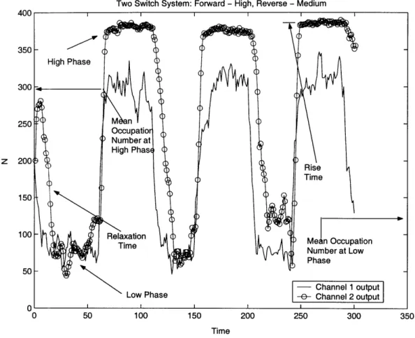
Two Switch System: Forward - High, Reverse - Medium

z

0 50 100 150 200 250 300 350

Time

Figure 2-1: The figure depicts a sample trajectory in which the various terms used to describe various components under analysis are labeled.

* Execute reactions: With these and in place, update the state vectors and increment time

The outputs of the algorithms are analysed as time-dependent trajectories. In the analysis of the trajectories, Figure 2.1 introduces several relevant terms used

throughout the discussion.

2.2 Mutual Information

Given the above method to simulate the dynamics of the enzymatic switches, and given that the modeled switching networks are fundamentally related to the incorpo-ration and transfer of information from the outside of the cell to the inside of the cell

as well as within the inside of the cell itslef, an important next step is determining the signal processing characteristics of the enzymatic switches. In particular we would like to quantitate the fidelity of the signaling procedure; that is, given the output trajectory of a given depth channel, we would like to know how much one random variable tells about the other. Recalling the work of C.E. Shannon, we define the quantity of nmlutual information [4] between two random variables as:

I(X

IY)

x y

where the quantities p(x) and p(y) are the probabilities that the random variables X and Y have values X=x and Y=y.

Some properties of mutual information:

* I(X Y) = I(Y X)

* I(X Y) = 0 if X and Y are independent random variables

* I(X -Y) = H(X) - H(X Y) where H is the Shannon entropy of the random variable signals

The third of the properties above in particular places a constraint on our models. In order that the mutual information not be affected by artifacts such as relative time spent in high and low phase, we run simulations with fixed ratios between the time spent in high phase and the total simulation time.

Armed with a method of simulating the biochemical dynamics and a method to quantitate the effectiveness of signaling, we now present our results that make use of the entire set of tools developed to simulate fabricated switching networks.

Chapter 3

Feedforward and Feedback Models:

The Two-Level Switch Cascade

Following specification of the model and implementation of the Gillespie algorithm for the case of a single enzymatic switch, the computer programs were modified to allow for various multiple phosphorylation schemes whose results are detailed below: i) double phosphorylation of each enzyme molecule (with the constituent reactions termed 'breadth channels'), in which the MAPK species undergoing covalent modifi-cations display two not necessarily identical phosphorylation sites where the output species is the doubly-phosphorylated MAPK-PP species, ii) double phosphorylation in stepwise fashion (with the constituent reactions termed 'depth channels'), in which the output of the first enzymatic switch channel is fed into a second enzymatic switch as its catalysing agent, iii) quadruple phosphorylation in stepwise fashion in which the motif presented in (ii) is developed further to include two additional depth channels;

see Figure 3.1 for illustrations of the three tasks. It is important to note that the n-phosphorylation case is computationally tractable within certain regions of parameter

space, however are of little biological relevance except to establish an upper bound on the number of depth channels needed to maximise the utility of the cyclic switch ar-chitecture. For each phosphorylation scheme we examine the effects of sweeping over different dimensions of parameter space - namely the number of molecules of species participating in the reaction network (N) and the different velocities characterising

the turnover rates between the constituent species (V).

3.1 Double Phosphorylation- Depth Channels

The double phosphorylation in parallel uses the model that the output of the first enzymatic switch is precisely the enzyme species that catalyses the phosphorylation of the substrate in the second enzymatic switch; that is to say the output of the first enzymatic switch plays the same input role for the second switch channel as the original environmental signal played for the first switch. Thus we can see that the information flowing through the reaction network is propagated via changes in the velocities of the forward reaction of each switch and is manifest in the amount of phosphorylated species produced by the second enzymatic switch.

Having implemented the model, we are now ready to perform our sweeps over parameter space to study the effects of altered reaction velocities and species numbers on the dynamics of the two-switch system.

3.1.1 Dependence on Forward and Reverse Reaction

Veloci-ties

Let us consider the case of the reaction velocities first. The first task in studying the dependence on the various reaction velocities the second switch can be tuned to is to fix the reaction velocities of the first switch in the cascade such that the first step of the network is operating in its dynamical range. Rather than manually probing the space of reaction velocities, we appeal to previous work carried out by Kueh and Mirny (reference poster) in which they describe a 'horseshoe' region of optimal information transfer for the case of a single enzymatic switch governed by the same underlying stochastic processes at play here. Using these results, we choose velocities at or near the middle of the dynamical range of each type of velocity (that is, the forward velocity with the environmental signal off, the forward velocity with environmental signal on, and the reverse velocity); the forward velocity with signal

off is fixed at 70, the forward velocity with signal on is fixed at 130, and the reverse velocity is fixed at 100 and all the first switches in the study use these values. Since the velocities of the reaction network also depend on the species concentrations, we will also constrain the total number of reacting species at 800, distributed equally a priori among the four types (unphosphorylated and phosphorylated species for each switch times two switches present in the model).

Having fixed the velocity characteristics of the first switch, we can study the effects of tuning the velocity characteristics of the second switch. Recall that the

Michaelis-Menten equation gives the reaction velocity as:

Vi = ki + [x ] (3.1)

Ki+ [i]

where [xi] and [x2] are the concentrations of the enzyme and substrate respectively

(in our simulations we substitute enzyme and substrate concentrations for the actual number of enzymes and substrate present, the number is referred to as the occupation

number of that particular state), ki is the chemical rate constant of the ith type

of reaction (i.e., either forward or reverse), and Ki is the corresponding Michaelis constant. Since [xi] is precisely the output of the first switch channel and thus an exogenous parameter with respect to the second switch's dynamics and [x2] is precisely

the unphosphorylated species of the output of the second switch and thus a dynamical variable in our network rather than a tunable parameter to be swept over, our sweep over biologically relevant forward and reverse reaction velocities is in actuality a sweep over relevant chemical rate constants. To reveal the effects of the various rate constants on the output of the second switch channel, let us consider several concrete examples sampled from different regions of parameter space. There are 3 broad subspaces to speak of for each type of velocity: the 'high', 'medium', and 'low' regions; thus there are 9 regions to consider made up of all the possible combinations of forward and reverse velocity subspaces. The explanation of the dynamics of these two-switch systems carry over naturally to explanations of all the various scenarios encountered by the networks.

41 3. 3( 2

z2

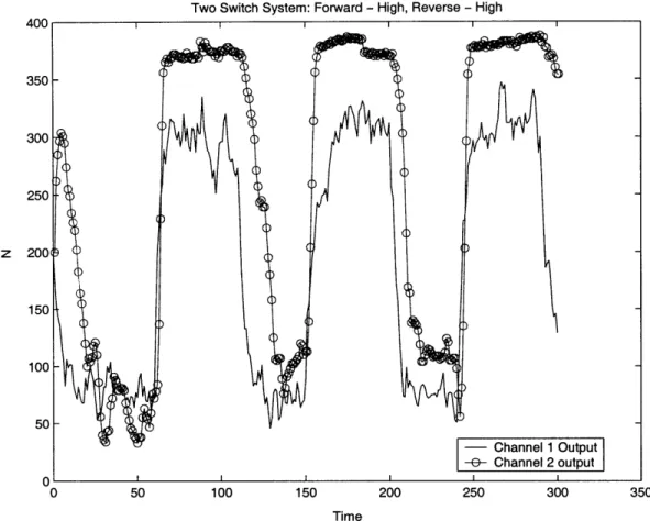
Two Switch System: Forward - High, Reverse - High

0 50 100 150 200 250 300 350

Time

Figure 3-1: The figure depicts a trajectory in which the forward and reverse velocities are in the 100) range.

3.1.2 Forward- High, Reverse- High

A typical trajectory for a reaction output is presented in Figure 3.1. In the doubly high region of parameter space, we witness an output with relatively low levels of noise overlaid upon the original signal and a rise time of 3 time steps, compared to the rise time of the original environmental signal itself which is defined as 1 time step. Furthermore, as a metric to determine the switch channel's effectiveness in serving as a low pass filter, the standard deviation of the stochastic fluctuations about the mean occupation number of = 377, the high phase of the switch channel output, is /sigma = 5.6620. For comparison the same parameters for the output of the first switch channel yield a standard deviation of 15.8668 about a mean occupation number at high phase of 298. Thus we see that in the 'forward-high, reverse-high'

regime for the second switch, the fluctuations about the mean value at high phase are more tightly constrained indicating a smoother profile and thus enhanced capacity for averaging over rapid, high-magnitude fluctuations - the very signature of low pass filtering.

As a quantitative measurement of the increased fidelity of the output of the second depth channel compared to the first we examine the mutual information between the initial square wave environmental signal and outputs of the two switches. We see that

the mutual information between the initial input and the output of the first depth

channel, averaged over 10 trials, is 0.8303. The corresponding mutual information measurement between the initial input and output of the second channel is boosted to 0.8938.

Thus in the 'forward-high, reverse-high' regime we observe a boost in signal strength from the first depth channel to the second depth channel (the mean oc-cupation number at high phase is boosted from 297 to 377), a tighter constraint on stochastically-driven fluctuations about this mean (standard deviations is cut from 15.8668 to 5.6220) consistent with low pass filtering behaviour, as well as a jump in the mutual information between the environmental signal and output of the second

depth channel versus the mutual information between the initial input and output of

the first depth channel.

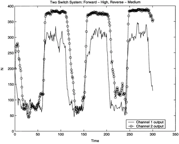
3.1.3 Forward- High, Reverse- Medium

A typical trajectory for a reaction output in the 'forward - high, reverse - medium' regime is presented in Figure 3.2. In examining the noise characteristics of the tra-jectory with respect to the above reaction parameter scheme, we notice a slight dete-rioration in the second switch channel's ability in filtering out high frequency noise, a deterioration that will manifest itself in a slightly decreased mutual information reading. While the rise time of the output signal remains sharp in accordance with

the characteristic rise time of the original input signal, the fluctuations about the

mean value at the high phase of the signal are greater in magnitude and frequency: using our standard deviation metric, cr is computed to be 8.3766 about a mean value

Two Switch System: Forward - High, Reverse - Medium

z

0 50 100 150 200 250 300 350 Time

Figure 3-2: The forward velocity hovers in the 100 range, whereas the reverse velocity is set at 50.

of 374. Despite this looser fit about the mean in the output of the second depth channel, its ability to dimish the magnitude of fluctuations is evident when compared to standard deviation of the output of the first channel with respect to its high phase mean occupation number: = 17.4182 about a mean p of 295.

With respect to the fidelity of the signaling process, the mutual information be-tween the input environmental square wave and the output of the first switch is 0.8686, whereas between the environmental input and output of the second switch the mutual information measures 0.8826. In this 'forward - high, reverse - medium'

region of parameter space, we observe all the qualitative features novel to secondary depth channels found above in the 'forward - high, reverse - high' region, but to a diminshed degree. The reduction in stochastic fluctuations about mean values stands at 48% in the above region of parameter space, where in the current region the re-duction is 35%. Furthermore the boost in mutual information in the above region was 7.6% versus the more anaemic 1.6% exhibited by the current reaction scheme. Nevertheless the current scheme did produce a gain in signal amplitude of 1.26, just as in the above scheme.

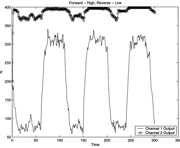
3.1.4 Forward- High, Reverse- Low

In figure 3.3, we see a sample trajectory in the 'forward - high, reverse - low' region of parameter space. Due to the forward velocity's dominance the kinetics of the reaction in the second switch channel, the occupation numbers of the second channel's output signal remains near the saturated high phase values, leading to smaller fluctuations about the high phase mean value but at the cost of diminshed mutual information and thus signaling fidelity. At the high phase of the output signal of the second reaction channel, the standard deviation is 1.j4032 about a mean occupation number of 395; the ocupation numbers thus exhibit a characteristic fluctuation of <1% about the mean, compared to 1.5% in the 'forward - high, reverse - high' and 2.2% in the 'foward - high, reverse - medium' regions. This fluctuation must furthremore be compared against the output of the first channel, which yields a a of 15.2299 about a mean output; occupation number of 297. With respect to the signaling fidelity in the

Forward - High, Reverse - Low

z

50 Time

Figure 3-3: Here the forward velocity is again tuned to be within a band centred at 100, whereas the reverse velocity is tuned down to 20.

regime, however, the mutual information between the initial environmental input and first output is 0.8383 whereas with the second switch's output is 0.6189, representing a 26% drop in mutual information; this is the cost for the greatly increased low-pass filtering behaviour. The gain in the signal is 1.33.

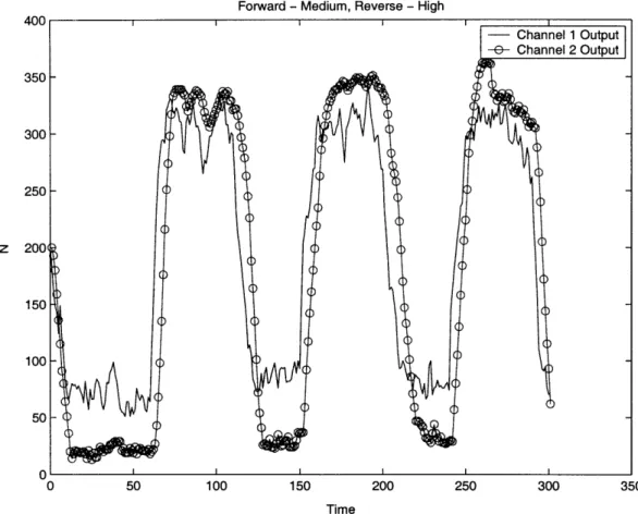
3.1.5 Forward- Medium, Reverse- High

The examination of this region of parameters will lead us to the central finding of the study of velocity (or equivalently the kinetc rate) dependece of the switching dy-namics: that the mutual information content rests on the difference between forward and reverse velocities, ceteris paribus. To this end let us examine several trajectories of this first opportunity in paraeter space to study the effects of the role reversal between forward and reverse velocity. The result comes as no surprise: if the reverse velocity is tuned such that Vreverse

»

First let us consider the case in which the forward velocity and reverse velocity are different by a factor of a small multiplicative constant on the order of unity, such as the situation depicted in Figure 3.4. Under these conditions we can carry out an analysis of standard deviations and gains to characterise the signal performance through the switch. We observe that in this subregion of parameter space a yields an average value of 8.1781 about a mean of 360. Compare these numbers against the output signal from the first depth channel which gives a reference standard deviation of 16.4944 about the mean output occupation number of 291; the gain in the second switch is thus 1.24. With these parameters, ranging in the low end of the reverse velocity's high region, the second switch is able to boost the mutual information content between its output and the initial square wave input from the 0.8293 measured between the input and first switch's output to 0.8359.

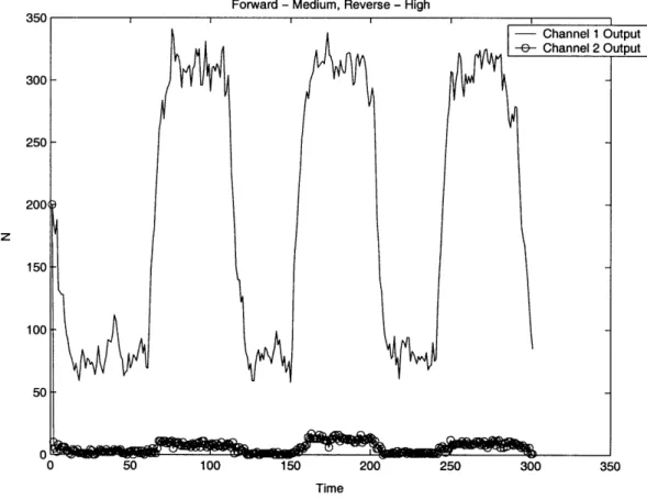
The next step, however, is taken when the reverse kinetic rate is tuned to a value such that the reverse velocity overwhelms the forward velocity in governing the switch dynamics. Such a trajectory is offered in Figure 3.5. As the reverse velocity

Forward - Medium, Reverse - High 4UU 350 300 250 z 200 150 100 50 n 0 50 100 150 200 250 300 350 Time

Figure 3-4: The figure allows us to see the first shift in forward velocity as its band is now centred at 50, whereas the reverse velocity is set at 100.

is tuned to higher and higher values, we observe that output formation in the second switch becomes exceedingly improbable, even with stochastic fluctuations, and thus information transfer is made impossible. The rate of decay in signaling fidelity with respect to this reverse kinetic rate tuning is detailed in Figure 3.6.

3.1.6 Forward- Medium, Reverse- Medium

The examination of the 'middle' regions in both parameters represents the most problematic situation in terms of defining the boundaries of the parameters to be swept over. To complicate matters further we again see a sharp drop-off in the value of the mutual information calcuations for all reverse rates in this region of parameter space. Since we gain no new insight from an examination of this region of parameter

Forward - Medium, Reverse - High 350 300 250 200 z 150 100 50 0 ( Time

Figure 3-5: To demonstrate the 'quenching' effect of very high reverse velocities, we

tune it to 1000. It is important to note that the data here allows us to conclude that

the difference between the forward and reverse velocities determine the dynamics; a similar trajectory could have been generated in the 'forward - high, reverse - high' regime if the reverse velocity were set very high even with a high forward velocity.

Mutual Information as a Function of Reverse Kinetic Rate in 'medium' Regime 0.8 C 0 co E 0.75 No C 0.7 0.65 0 1 2 3 4 5 6 7 8 9 10 Index

Figure 3-6: The appearance of a sharp drop in mutual information content appears for all reverse velocities in a wide band in the middle of the forward velocity sweep. A section of that is given here with error bars indicating the variability of the information loss.

space, and since the reasoning behind the data presented above carries completely naturally to the other possible velocity pairings, we omit detailed discussion of the results and instead direct attention toward Figures 3.7, 3.8, and 3.9, which present

summary findings on the various reaction trajectories.

3.2 Dependence on Species Number

The dynamics of the stochastic switches are not dependent on the chemical parameters of the underlying equations alone, but also on the total number of molecules of each type undergoing the chemical reactions. The dependence on the number N of each

.~~~~~~ I 7 / I I I I I I I I I I I I I I I I I _ _ r-

ZZ

,J

z

l- I I I ~~~~~~~~~~~~~~~~~~~~~~~~~~~~~~I I I ~~~~~~~~~~~~~~~~~~~~~~~~~~~~~~~~~~~~I _I l

An

A

I

~~~~~~~~~~~~~~~~~~~II

I- I

I

--.

I

~~~~~~~~~

~~~~~I

A

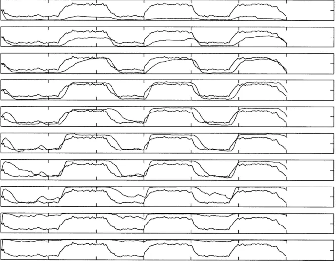
Figure 3-7: We can track the evolution of the second switch response as parametrised by the forward rate constant. The second switch response has little phosphorylated product when the forward rate is very low, but as the rate is tuned to higher values we see the formation of square wave signal outputs. This continues until the rate is tuned to too high a value which causes total saturation of the occupation numbers in high phase.

I I I I I I I I A I I I I

-1

A

A

A

A

A

Figure 3-8: We again track the evolution of the second switch response as

parametrised by the forward rate constant, but this time against a smaller reverse

... ~~~~~~~~~~~ I I I

A

A

A

A

Figure 3-9: We again track the evolution of the second switch response as

parametrised by the reverse rate constant, to give an indication of the other

type of reactant is gauged in a manner similar to the study of the dependence on the kinetic rate parameters: low-pass filtering and signal gains are measured directly from the trajectories themselves and are computed as the average values over several trials for each N, while the mutual information is obtained by overlapping the trajectories against the reference signal as required by the definition of mutual information and then averaged. It is important to note that the simulations here present only the N dependence of the switches, all velocities and Michaelis constants are kept constant for all the linked switches.

3.2.1

Low N

In the extremely low region of N's parameter space, the ability of the switch to act as a low-pass filter, the gains in signal strength that underly the ability of the cascades to act as amplifiers, and the throughput mutual information referenced against the environmental square wave signal all exhibit diminished quality. With the stochastic fluctuations about the mean value of the high phase of the depth channel outputs on the order of the mean occupation number itself, the use of standard deviations and mean values to characterise the low-pass filtering behaviour and computing gains in signal strength are rendered meaningless and we are forced to conclude that the switches simply do not exhibit such behaviour at such low molecule numbers. With

such great variability in the trajectories, it is no surprise that the throughput mutual

information averages to 0.2189.

3.2.2

Middle N

The middle region of N represents the optimal region of information transfer, as can be seen qualitatively from the trajectories presented in the second row of Figure (9 trj's). The region in parameter space has enough chemically reacting components to ensure that the stochastic fluctuations are characteristically one or two orders of

mangitude smaller than the mean occupation numbers of the output signals at high

meaningfully propagate information from upstream reactions through the network.

3.2.3 High N

The high region of N represents the another drop-off in the ability of the network to

propagate information. Rather than the stochastic fluctuations, however, the problem

here lies with the fact that the output occupation number fails to reach a saturation point due to the high number of molecules available for phosphorylation. Thus the trajectories exhibit sawtooth curve system responses rather than square waves.

The mutual information as a function of the species number N is depicted in Figure 3.8. We see that in the first switch there is a marked optimal region of information transfer manifested in the relatively sharp peak in the profile. In the second switch, however, the mutual information drop-off as a function of the log of the species number is far more shallow, indicating a high degree of robustness

3.2.4 Mixed Number Cascades

Having determined the channel characteristics for switches casacaded in a two depth-dimensional series with the same N for each switch, we must take up the task of studying the interactions of switches with different values of N. Namely, as an illus-tration that order of magnitude differences in N between switches disallow efficient transfer of information, we present simulation results in which:

* N = 25 switch feeds into N = 125 and N = 1250 switches

* N = 125 switch feeds into N = 25 and N = 1250 switches

* N = 1250 switch feeds into N = 25 and N = 125 switches The drop-off in the mutual information is evident in Table 3.1.

3.2.5 N = 25

N = 125, 1250 Switches

Figure 3.10 depicts the ability of a switch involving 25 molecules to phosphorylate switch channels with 125 and 1250 molecules repsectively. Since the velocity of the

Mutual Information as a Function of Species Number

-- Channel 1 Output

I

Chnnel

9 ritnt

It

v0 1 2 3 4 5 6 7 8

log(N)

Figure 3-10: The figure implies the important idea that even with higher numbers of interacting species making up the second switch, the information transfer through the switch is robust against the increase unlike the single switch case.

Table 3.1: Table depicting switches of different N

the signal processing characteristics of several enzymatic N -+ I(XIY), 1st type I(XIY),2nd type

25 125 1250 0.3112 0.5775 0.1555 0.1761 0.3378 0.1938 0.9 0.8 0.7 x . 0 -0.6 0.5 0.4 0.3 0.2 0.1 n I -. I _ _ _

N = 25 Switch -e N = 125, N = 1250 Switches

z

0 50 100 150 200 250 300 350 Time

Figure 3-11: The reverse reactions dominate the channels.

turnover from unphosphorylated to phosphorylated species for the second switch is directly proportional to the occupation numbers of the output of the first switch, and since the output of the first switch is constrained to be in the low N regime, the reverse velocity dominates the dynamics of the switches for both N = 125 and N = 1250. Furthermore the N = 25 switch fails to propagate mutual information in an optimal manner to begin with, as evidenced from above considerations. The result is that for each of the second switch's forward reaction is largely quenched, the output occupation numbers are very low, and the phosphorylated forms appear mainly due

to stochastic fluctuations in the network rather than due to the driving force supplied

N = 125 Switch -- N = 25, N = 1250 Switches 1bUU 1000 500 n 0 50 100 150 200 250 300 350 Time

Figure 3-12: The switches misalign with respect to the middle N value.

3.2.6

N = 125 -

N = 25, 1250 Switches

The intermediate-value N switch providing the enzyme for the low and high N value switches exhibits both problems that the mixed number cascades have when the N =125 switch feeds the N = 25 switch, the forward velocity so dominates the dynamics that the N == 25 switch remains locked in high phase with stochastic fluctuations driving the dephosphorylation reaction. With the N = 125 switch feeding into the N = 1250 switch we observe the opposite problem, which in principle is the same problem faced in the N = 25 case in the first switch - the N = 125 switch does not support a high enough velocity to interconvert the unphosphorylated forms to remain phosphorylated for long enough to pass through meaningful information from the original environmental signal, hence the sawtooth-shaped trajectories.

---3.2.7

N = 1250 -

N = 25, 125 Switches

The N = 1250 switch acting as the input to the N = 25 and N = 125 produces the expected saturation behaviour with respect to the two switch outputs. The transient behaviour in the first 60 time units of the N = 25 and 125 switches is a result of the initial enzyme number of the first switch being so high ( 1250), thus driving the second switch to saturation; when the N = 1250 switch equilibriates to its low phase, the N = 25 and 125 channels exhibit a shart drop-off in the response. Once the first channel hops to high phase again, both types of second switch are quickly driven to saturation. When the first channel transitions to its low phase and back to high phase from this instance onward, however, the first channel output is not in the low phase for long enough time before switching back to high phase for the N = 25 or 125 switch outputs to respond by also switching to low phase.

N = 1250 Switch - N = 25, N = 125 Switches

z

0 50 100 150 200 250 300 350 Time

Figure 3-13: The N = 1250 overdrives the system and locks the switches into high phase.

Chapter 4

Feedforward Simulation Results:

Probing the Depth Channels

The simulations presented here represents a different type of model as the outputs of the various switch channels are fed immediately forward as catalysts of the chemical reaction characterising the next switch in the cascade. The result is that there is no 'real-time' feedback into a switch from the downstream dynamics (the physical picture being that downstream sequestration of a given enzyme species results in keeping the dephosphorylation reaction velocity of that enzyme unchanged). We now introduce our model in a concrete manner and analyse the output from the simulations.

4.1 Dependence on Depth Dimension

The purpose of this section is to examine the effects of additional depth channels, labelled by an index d, to the system, especially with regard to information transfer properties. While the reaction velocities, numbers of participating molecules, and Michaelis constants of each switch could all be tuned to various values, the combina-torial problem is outside the scope of this paper. We will first analyse the trajectories

of the outputs of the additional depth channels and then examine the mutual infor-mation properties.

Time Series of 4 Depth Channels in Series - Type 1 Trajectory a) 0_c) 0 E 06 0 50 100 150 200 250 300 Time

Figure 4-1: The Type 1 trajectory only involves square wave responses in all switch outputs. Type 1 switches are able to achieve higher signaling fidelity with respect to the reference environmental signal farther down the cascaded network.

4.1.1 Trajectories

In examining the outputs of the switching cascades, we observe that thehere are two types of trajectories. Type 1 trajectories, such as shown in Figure 4.1, present the

motif of square waves generating square wave responses in their downstream switches. Type 2 trajectories, such as shown in Figures 3.12 and 3.13, exhibit a qualitatively different behaviour in which the switch response either develops or loses a dynamically generated 'memory'; the presence of a switch 'memory' is marked by the failure of upstream shifts from high phase to low phase to affect the phase of downstream switches.

Let us examine the Type 1 trajectory more closely. First we perform the usual analysis of computing standard deviations of the output occupation numbers about

Time Series of 4 Depth Channels in Series - Type 2: Dynamically Generated Memory Gain Coa) 03 E 0 0 50 100 150 200 250 300 Time

Figure 4-2: Type 2 switches, unlike Type 1 switches, see their output experience a qualitative change over time. Even as the upstream signals oscillate between high and low phases, the system response in the downstream switches transition from oscillatory to remaining locked in one phase or the other, which we understand as a generated 'memory'. The trajectory here represents a dynamically-generated memory gain.

the mean at high phase, the results of which are tabulated in Table 3.2. We see the characteristic monotonic reduction of fluctuations from the d = 1 to d = 2, 3, and 4 switch channels as one low pass filter feeds its output signal into another. Thus we see that the same reasoning behind the dynamics of the two-level switching system carries over naturally to the four-level system for Type 1 trajectories.

The Type 2 trajectories the same low-pass filtering behaviour with each additional dimension in the cascade. The difference, however, is the appearance of a 'memory' in the fourth switch output. The transition from Type 1 to Type 2 behaviour is

Time Series of 4 Depth Channels in Series - Type 2: Dynamically Generated Memory Loss

0 50 100 150 200 250 300 Time

Figure 4-3: This Type 2 switch represents a dynamical loss of 'memory'.

a)

C)

a) E

Table 4.1: Table depicting the signal processing characteristics of several enzymatic switches linked via a feedforward model.

Depth Channel p 0t 0

determined by the kinetics of the original d = 1 switch (and thus most likely also by the kinetics of each switch in the cascade).

4.1.2 Mutual Information

Figure 4.4 presents the trial-averaged mutual information data between the output of the nth depth channel and the reference environmental signal. In this region of parameter space we see a linear decay of the mutual information with respect to the depth channel number. Using the MATLAB curve fitting tools, we find that the dependence in this linear regime is given by:

I(X[Y) = -0.1555d + 0.9856

(4.1)

where I(XIY) is the mutual information and d is the depth channel; it is important to note that I(X[Y) [0,1], whereas d E Z+. The residuals of the curve-fitting can be found also in 4.4.

4.1.3

Sensitivity Analysis for Large d

Before moving to the 'asymptotic' case, we offer results on the sensitivity of the multi-step phosphorylation scheme to both rate constants as well as species numbers.

1 0.8 0.6 0.4 0.2 1 0.2 0.1 0 -0.1 -0.2 1.5 1 2 1.5 2.5 residuals 2 2.5 3.5 3 4 3.5

Figure 4-4: The mutual information exhibits a linear fall-off as a function of the depth channel when considering the four-switch cascade. The residuals to the fitted line are also given above.

Four Switch Cascade: Mutual Information as a Function of Channel Number

I(XlY) = - 096

- Mutual info data | -- Linear fit

Switch Number

I I I II

Linear: norm of residuals = 0.02852 I

-Linear: norm of residuals = 0.02852

I I I I I

Mutual Information as a Function of Species Number U. 0.6 0.5 0.4 >.. X 0.3 0.2 0.1 13 v 4.5 5 5.5 6 6.5 7 7.5 log(N)

Figure 4-5: The mutual information exhibits an increasingly decaying both a function of the species number as well as the depth channel.

8 8.5 9

Mutual Information as a Function of Forward Rate Constant U. 0.75 0.7 0.65 0.6 >..

x

Forward Rate Constant

Figure 4-6: Like with the above situation, here also the mutual information decays, as the sweep moves beyond the dynamical range of the velocities and as the trajectory occurs in a later trajectory.

i.~

2

Output

-- Channel 2 Output Channel 3 Output 4-, . | 4 Channel 4

//\

a_

,

~

~

~

~~~

4.1.4 The Asymptotic Case

For the sake of completeness, we present the mutual information as a function of the depth channel number. The procedure involved extended the method used above to generate 4-level systems to the generalised N-level system.

Using the MATLAB curve fitting tool, we compare power law and exponential decay models for the mutual information dependence on depth channel. The power law model, whose fitting statistics are presented in Figure 4.8, is given by:

I(XIY) = 2.051d- 1- 1.176 (4.2)

The exponential decay model, which the fitting statistics predict over the power law model, is given by:

d

I(XIY ) = 1.068 * e- 4 (4.3)

Asymptotic Behaviour of Cascading: Mutual Information as a Function of Depth Channel

2 3 4 5 6 7 8 9

Switch Number

Figure 4-7: We see that the linear behaviour in the four-switch region is an ap-proximation to a nonlinear behaviour in the mutual information as a function of the channel number. 0.9 0.8 0.7 0.6 0.5 0.4 0.3 0.2 0.1 1

Mutual Information: Power Law Fit 0.9 0.8 0.7 .- 0.6 x- 0.5 0.4 0.3 0.2 0.08 0.06 0.04 0.02 0 -0.02 -0.04 -0.06 1 2 3 4 5 6 7 8 9 Depth Channel Residuals 1 2 3 4 5 6 7 8

Figure 4-8: The first of two competing models to describe the nonlinear response of the mutual information to the depth channel is a power law equation, whose fitting statistics and residuals are given above.

I I I I I I I I I 9 _ _ _ _

Mutual Information: Exponential Decay Fit 1 2 3 4 5 6 7 8 9 2 3 4 Depth Channel Residuals 5 6 7 8 9

Figure 4-9: The exponential decay model yields a higher R-square value, and smaller residuals as seen above.

0.8 0.7 0.6 0.5 0.4 0.3 0.2 0.1 0.08 0.06 0.04 0.02 0 -0.02 -0.04 1

Chapter 5

Conclusions

The stochastic dynamics of enzymatic switches display novel features that are of interest to both theoretical biology as well as theoretical physics, as they bear on the abstract fundamentals of the practise of cellular communication and provide an important complex system to model using the machinery of statistical mechanics and information theory.

5.1 Low-Pass Filtering

Analysis of the trajectories reveals that whether or not feedback effects in the cou-pled switch network are included, the individual switch elements act as low pass filters, which in the context of our biochemical reactions means that the variability in the occupation numbers of the output state of each successive switch is reduced at each stage. This ability to reduce variability, when manifest in further downstream switches, is likely to be the same mechanism that results in the dynamical memory gain and loss in the switch responses. In the cases of memory, the downstream swith-ces exhibit a highly nonlinear reponse to the throughput signal, sending the output occupation numbers to either high phase or low phase and then the reduction in

variability locks the phase of the switch output, thereby rendering it unresponsive to further upstream oscillations.