A dynamic term structure model of Central Bank policy

A Dynamic Term Structure Model of Central

Bank Policy

by

Shawn W. Staker

AUG 0 7 2009

LIBRARIES

Submitted to the Department of Electrical Engineering and Computer

Science

in partial fulfillment of the requirements for the degree of

Doctor of Philosophy

at the

MASSACHUSETTS INSTITUTE OF TECHNOLOGY

June 2009

@ Massachusetts Institute of Technology 2009. All rights reserved.

A uthor ... .

Department of Electrical Engineering and Computer Science

June5, 2009

C ertified by ....

-

---Leonid Kogan

Nippon Telephone and Telegraph Professor of Management

Thesis Supervisor

Accepted by...

.. ...

...

Terry P. Orlando

Chairman, Department Committee on Graduate Theses

A Dynamic Term Structure Model of Central Bank Policy

by

Shawn W. Staker

Submitted to the Department of Electrical Engineering and Computer Science on June 5, 2009, in partial fulfillment of the

requirements for the degree of Doctor of Philosophy

Abstract

This thesis investigates the implications of explicitly modeling the monetary policy of the Central Bank within a Dynamic Term Structure Model (DTSM). We follow Piazzesi (2005) and implement monetary policy by including the Fed target rate as a state variable. The discontinuous target dynamics are accurately modeled via a non-linear switching process, while still maintaining affine requirements under the pricing measure ensuring tractability. To ensure a flexible risk specification we turn to the parametrization of Cheridito et al (2007), with extensions to the target jump process. Model parameters are estimated via a simulated maximum likelihood es-timation scheme with importance sampling. A Bayesian particle filter is used as a robustness check, and it's use for static parameter estimation in a DTSM framework is explored.

Our results support those in Piazzesi (2005), revealing a substantial improvement in pricing errors especially on the short end of the yield curve. The model construction provides a natural framework to inspect monetary policy information embedded in yields, which is found to be substantial. We find the addition of the target rate greatly improves the model's ability to explain excess return. An ability which is increased with the inclusion of the full term structure of target rates, as measured from Fed future contracts. We postulate the improved performance is due to the target as a proxy for short term rates, and a conduit to express the information content of the term structure of target rates.

Thesis Supervisor: Leonid Kogan

Acknowledgments

I would like to thank my research advisor Leonid Kogan for his continual support and never ending patience. I am also grateful to the members of my research committee: Munther Dahleh, Scott Joslin, and John Tsitsiklis. Much of my work, and most of my sanity, is due to the invaluable and extensive discussions with Scott Joslin. Teaching for Munther Dahleh and John Tsitsiklis are highlights of my MIT education, providing experiences which have shown me my way forward.

I owe a special debt to Andrew Lo for providing me with office space at the Laboratory for Financial Engineering. A unique collaborative center, supporting a wide range of bright students and exciting research. Finally if it wasn't for fellow classmate Amir Khandani, I would have driven myself mad with talk of Q measures. Though the trials and tribulations associated with this thesis have marked my time at MIT, the meeting of Tufool Al-Nuaimi has marked my life. I owe her more than I can ever repay, and love her more than I can say. My academic accomplishments pail in comparison to the pride I feel in starting a new chapter of my life with the woman I love. Ahibik b'kul qalbee.

Contents

1 Introduction

2 Dynamic Term Structure Models

2.1 Mathematical Foundation ... 2.2 Affine Term Structure Models ...

3 DTSM of Central Bank Policy

3.1 M otivation ... 3.2 Model Construction ...

3.2.1 Latent State Space ... 3.2.2 Jump Process ... 3.2.3 Change of Measure ... 3.2.4 Bond Pricing Coefficients.... 3.3 Estimation ...

3.3.1 Simulated Maximum Likelihood 3.3.2 Particle Filtering ...

3.4 Market Data. ... 3.4.1 FOMC Data...

3.4.2 Libor & Swaps . . . . with. . .

. . .

. . .

Importance

... 0.

3.4.3 Fed Future Contracts

4 Results & Performance

4.1 Estim ation Results ... 7 23 23 26 31 31 35 36 38 40 43 46 47 50 52 53 53 Sampling ... 57 57 . . . . . . . . . . . . . . . . ...

4.2 Pricing Errors .. ... . .. ... . .. .. . . . ... . ... . .. .. 76

4.3 Yield Response to Shocks ... 83

4.4 Risk Premium ... 92

5 Conclusion 103

A Bond Pricing Accuracy Check 105

B Estimation 107

B.1 Simulated Maximum Likelihood ... .. 107

C Details on Model Extensions 109

C.1 A1(3) Benchmark ... 109

List of Figures

3-1 Monthly estimates of tracking error with respect to the Fed target rate.

Tracking error is difference in non-overlapping monthly averages of the Fed target and the Fed effective funds rates. Sample mean absolute tracking error 2.61 bp, sample vol 4.56 bp. . ... 33 3-2 Times Series of the Fed target rate, the intended overnight Fed funds

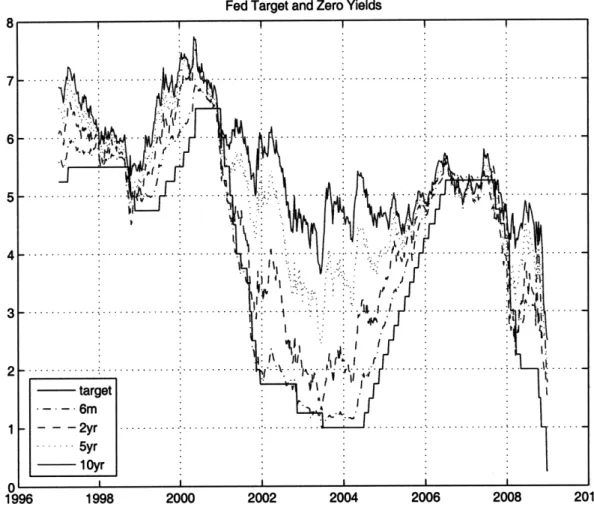
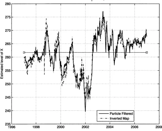
rate set by the FOMC. Changes to the target announced during sched-uled FOMC meetings (circle), changes to the target announced during unscheduled FOMC meetings (square). . ... 34 3-3 Histogram of changes to the Fed target ... 35 3-4 Time series of the Fed target and a subset of synthetic zero yields... 55 4-1 Estimated values of the stochastic volatility factor Xt. Horizontal bar

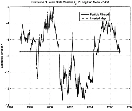
fixed at the P measurable long run mean of X1. . ... 60 4-2 Estimated values of the latent state variable X2 . Horizontal bar fixed

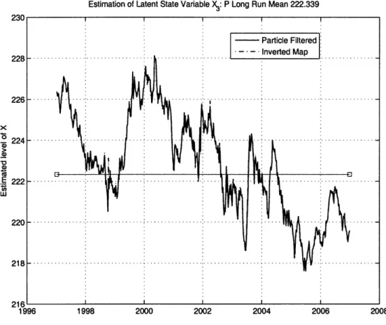
at the P measurable long run mean of X2. . . . . 61 4-3 Estimated values of the latent state variable Xt. Horizontal bar fixed

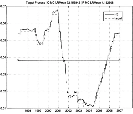
at the P measurable long run mean of X3. . . . . 62 4-4 Estimated values of the latent short rate r(Xt), and the observable Fed

target rate. ... 63

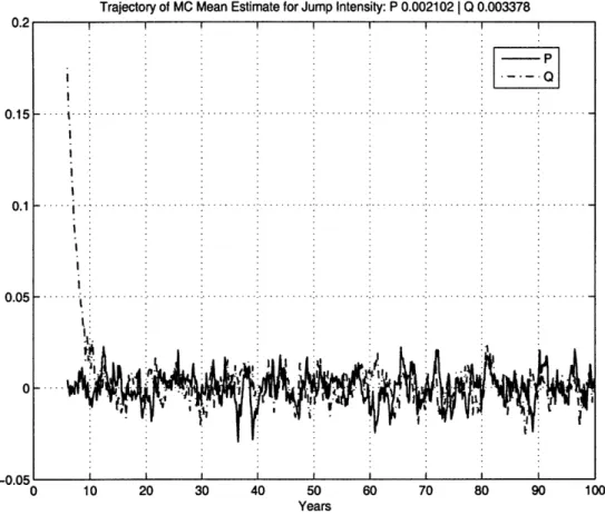
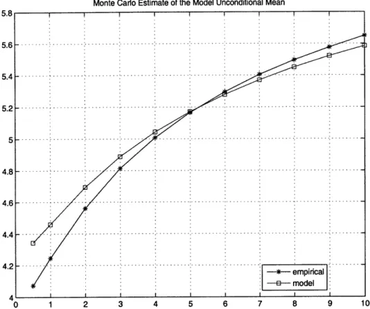
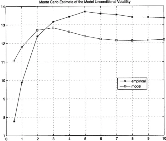
4-5 Monte Carlo verification of long run mean of jump intensity. ... 64 4-6 Monte Carlo estimate of model yields unconditional mean. ... . 65 4-7 Monte Carlo estimate of model yields unconditional volatility. .... 66 4-8 Monte Carlo estimate of model yields unconditional skew. ... . 67

4-9 Monte Carlo estimate of model yields unconditional kurtosis... 68 4-10 Monte Carlo draws of the short rate as a histogram. . ... 69 4-11 Short dated model predictions of target changes at the next FOMC

meeting. Estimates are maximum likelihood values via a Monte Carlo

generated distribution of 0. ... 70

4-12 Decomposition of future expected target changes over the next sched-uled FOMC meeting, where the y-axis is in units of 25 basis points. Fu-ture expected target changes are approximately equal to Et[AsS t]h.

Where the next scheduled meeting is at time s and h is the length of

the meeting... 72

4-13 Decomposition of future expected target changes over the next sched-uled FOMC meeting with respect to current yields. Future expected target changes are approximately equal to Et[Als > t]h. Where the next scheduled meeting is at time s and h is the length of the meeting. Correlation is the standard sample correlation on first differences. . . 73 4-14 A time series of out-of-sample pricing errors for near dated Fed Future

contracts ... ... 81

4-15 Time series of the number of 25 basis point jumps in the Fed target rate expected to occur at the next scheduled FOMC meeting. Model EQ[Jumps] are taken from the model using the optimal model param-eters of table 4.1. Market EQ[Jumps] are obtained by inverting the pricing relation for Fed future contracts. . ... 82 4-16 Loadings for the first three Principle Components of Yields. ... 83 4-17 Normalized pricing vector. Cx is normalized to display the response

to a 1 standard deviation shock. Co requires no such normalization. 85 4-18 Normalized pricing vector. Cx is normalized to display the response

to a 1 standard deviation shock. Co requires no such normalization. 86 4-19 Time series of model implied monetary policy shocks, as well as shocks

measured via Fed future contracts. Sample correlation of two measures is 0.7632 .. . . . . . . . ... .. 88

4-20 Response of Yields to shocks in monetary policy, as measured by unan-ticipated changes in the Fed target rate. . ... 91 4-21 Realized one year excess return on {2,3, ..., 9, 10} year bonds using

weekly sampled bond yields. Return calculations use overlapping

win-dows. ... 93

4-22 Model expected one year excess return on {2,3, ..., 9, 10} year bonds using weekly sampled bond yields. Return calculations use overlapping window s .. . . . . .. . . . ... 95 4-23 Explaining excess bond returns. The Benchmark is a A1(3) model

with no jump component. Ylds indicates the use of model parameters of table 4.1, which are estimated using yields only. ... 96 4-24 Plot of the term structure of target rates taken from Fed future

con-tracts during the 2000 turning point. Doted line is the actual Fed

target rate. ... 97

4-25 Plot of the term structure of target rates taken from Fed future con-tracts during the 2005 tightening cylce. Doted line is the actual Fed

target rate. ... 98

4-26 Explaining excess bond returns. The Benchmark is a A1(3) model

with no jump component. Ylds indicates the use of model parameters of table 4.1, which are estimated using yields only. Ylds & Futures represents model performance when yields and Fed future contracts are used to calibrate model parameters. . ... 99 4-27 Explaining excess bond returns via ordinary lease squares regression.

3PC are the three principle components of all yields of section 3.4.2. MM indicates the short dated 1 week money market rate. FF indicates the 1 month ahead Fed Future contract as described in section 3.4.3. 100

List of Tables

3.1 Table of changes to the target which were announced during unsched-uled FOMC meetings. Includes dates from January 1 1997 to January

1 2009 . . . . 35 3.2 _{Percent of total variation explained by the first k principle components,}

where the principle component decomposition is performed on yields (levels) and first differences of yields (changes). . ... 36

4.1 Point parameter estimates for model parameters of section 3.2. Esti-mates are calculated via the simulated maximum likelihood technique described in section 3.3.1. Sample period is from January 1997 to January 2007, including 521 weekly samples. Standard errors are com-puted via the product of outer gradients [3]. . ... . 59

4.2 Half-life of shocks for an equivalent diagonalized system of Xt. Specif-ically -log(0.5) A-1 , where A are the eigenvalues associated with the

drift matrix of Xt ... .. 60

4.3 Long Run Mean of Xt under the Q pricing measure, and the historical

measure P. ... 61

4.4 In-sample prediction errors of near dated target changes during sched-uled FOMC meetings. Maximum absolute prediction error is 25 basis

4.5 Point parameter estimates. Estimates are calculated via the simulated maximum likelihood technique described in section 3.3.1. Sample pe-riod is from January 1997 to January 2007, including 521 weekly sam-ples. Standard errors are computed via the product of outer gradients

[3]. ... .. 74

4.6 In sample pricing errors of yields in basis points. RMSE via map is found by observing the six month, two year, and ten year yields with no error and inverting the measurement equation. RMSE via Particle Filter is obtained by applying the Bayesian Particle Filter of section

3.3.2... 77

4.7 OLS estimates of the coefficients in eq(4.39). Heteroskedasticity-consistent White t-statistics in parentheses. ... .... . . . 90

A. 1 Monte Carlo estimates of pricing errors due to linearization of the jump term and normalization of the meeting schedule. Root mean squared errors (RMSE) in basis points (pb). MC-ODE is the RMSE of the difference between the MC yields and the ODE yields. . ... 106

C.1 Point parameter estimates for the A1(3) benchmark model. Estimates

are calculated via the simulated maximum likelihood technique de-scribed in section 3.3.1. Sample period is from January 1997 to January 2007, including 521 weekly samples. Standard errors are computed via the product of outer gradients [3]. ... . . . 112 C.2 Point parameter estimates for the target model with information

con-tent of the full term structure of target rates incorporated. Estimates are calculated via the simulated maximum likelihood technique de-scribed in section 3.3.1. Sample period is from January 1997 to January 2007, including 521 weekly samples. Standard errors are computed via the product of outer gradients [3]. ... . . . 113

C.3 In sample pricing errors for the target model with information content of the full term structure of target rates incorporated. RMSE via map is found by observing the six month, two year, and ten year yields with no error and inverting the measurement equation. RMSE via Particle Filter is obtained by applying the Bayesian Particle Filter of section 3.3.2 . . . . 114

Chapter 1

Introduction

This thesis investigates the implications of explicitly modeling the monetary policy of the Central Bank within a Dynamic Term Structure Model (DTSM). We follow Piazzesi (2005) and implement monetary policy by including the Fed target rate as a state variable. The discontinuous target dynamics are accurately modeled via a non-linear switching process, while still maintaining affine requirements under the pricing measure ensuring tractability. To ensure a flexible risk specification we turn to the parametrization of Cheridito et al (2007), with extensions to the target jump process. Model parameters are estimated via a simulated maximum likelihood es-timation scheme with importance sampling. A Bayesian particle filter is used as a robustness check, and it's use for static parameter estimation in a DTSM framework is explored.

Our results support those in Piazzesi (2005), revealing a substantial improvement in pricing errors especially on the short end of the yield curve. The model construction provides a natural framework to inspect monetary policy information embedded in yields, which is found to be substantial. We find the addition of the target rate greatly improves the model's ability to explain excess return. An ability which is increased with the inclusion of the full term structure of target rates, as measured from Fed future contracts. We postulate the improved performance is due to the target as a proxy for short term rates, and a conduit to express the information content of the term structure of target rates.

Motivation

Our motivation to explicitly include monetary policy into a term structure model stems from it's well established importance in the wider economy. Changes in the monetary base directly effect short term rates, and though various intermediaries effect everything from consumer credit to exchange rates. The Fed alters the monetary base to meet it's dual mandate of price stability and sustainable economic growth [36]. The Federal Reserve Bank maintains three controls for monetary policy, all with the purpose of influencing the daily Fed funds rate. The Fed funds rate is the overnight interest rate which depository institutions lend balances to other depository institutions. Based on this description a logical choose would be to use the Fed funds rate as a state variable reflecting monetary policy. Unfortunately the realized Funds rate has a number of adverse qualities, principally very high volatility which is found in many money market rates. As with many money market rates, spikes in the rates often appear due to known institutional constraints rather than economic drivers.

An alternative choice is to use the publicly announced Fed funds target rate, or target rate. This is the rate the Fed attempts to steer the funds rate toward via it's tools of monetary policy. The process in which the Fed conveys the target rate has evolved with the organization's view on transparency. In 1994 the Federal Open Market Committee (FOMC) began disclosing changes to it's policy stance. This evolved in 1995 to a full announcement of the current target level. Communication tools have evolved since then in an effort to increase transparency, notably in 2000 when the FOMC began to issue assessments on risks to it's dual mandate'. Due in part to data constraints, our analysis will be limited to a post 1995 time period where changes to the target rate are publicly announced. Besides the lack of volatility found in the funds rate, the target is appealing for two broad reasons. The first is the FOMC's ability to keep the funds rate close to the target rate, which is discussed in more detail in section 3.2. The second is the unique trait in that the target is not a market rate, thus it contains no risk premium. As such it may be seen as a proxy for other indicators of the economy, such as inflation or GDP. This fact will have

interesting implications for risk premium as discussed in section 4.4.

From a mathematical modeling perspective, the target possesses several unique characteristics with respect to other interest rates. Since 1994 the FOMC has adjusted the target rate in 25 basis point (bp) increments, and almost predominately at one of the eight annual FOMC meetings. Incorporating the unique discretized dynamics and the strong seasonality has the potential to greatly increase the model's ability to explain observed phenomenon.

From an econometric perspective there have been a number of recent studies lend-ing support to the importance of the Fed target. One of first studies on yield responses to changes in the target showed mixed results [16]. Once target changes were decom-posed into expected and unexpected changes studies found significant yield response even with long dated maturities [45]. That expected target changes should have no effect on yields, makes intuitive sense as this information has already been incorpo-rated into prices. The fact that unexpected target changes, or shocks, effect yields is a strong motivator for our study. Event studies also provide strong support of jumps during FOMC announcements, such as [34]. Finally more parametric mod-els have provided strong support in allowing interest rates to jump during FOMC announcements, see [43} and [42].

Literature Review

The reported work follows several themes in the current literature. Most notably are other published studies which explicitly model the Fed target rate within a term structure model. The most notable of which are [40], [50], and [51]. [40] investigate a Gaussian term structure model with Fed targeting, where deterministic Fed jumps are used. [50] build a finite state Markov Chain to characterize target changes, and find good predictability over a somewhat short sample period.

In particular our work can be seen as an extension of the model in [51], who uses an affine term structure model with conditionally Poisson jumps driving the target. Our model uses a richer specification for the jump process, combining a single time series with a non-linear switching mechanism to drive target jumps. Other

extensions include a more flexible parametric description of the pricing kernel, and an estimation scheme incorporating a variance reduction technique. We also exploit a Bayesian Particle filter for a robustness check, and explore it's use for parameter estimation. Finally our results focus more heavily on model risk premium, and it's response to the market's term structure of target rates.

Our modeling approach falls within the broad class of Dynamic Term Structure models (DTSM). To maintain tractability we transform the dynamics under the pric-ing measure which places the model under the affine variation of DTSM models, or Affine Term Structure Models (ATSM). [59] and [17] are early examples of term structcure models, which are now seen as specific examples of ATSMs. The seminal work which established the broad framework of ATSM models is found in [28] or [27]. Since then [19] and [20] further established the foundations of drift-diffusion ATSM models which exist today. This framework was extended to in [29] to accomidates Poisson type jumps. An excellent survey paper on ATSM models is found in [52], with an equivilant in the DTSM space available in [18]. Finally a comprehensive text book treatment of DTSM models with an empirical focus is found in [581.

Within ATSM modoels the pursuit of more flexible parametric specifications for risk premium has been an active subject. An appropriate starting point is the com-pletely affine price of risk specification in [19]. A slight adjustment in [23] was later coined semi-affine, followed by essentially affine in [24]. These variations have led to the fully flexible extended affine configuration of [12], which allows for a price of risk such that the state space under P and

Q

A key ingredient to any term structure model is the means to calibrate static model parameters to historical data, and possibly infer latent state variables. We will label all such issues under the umbrella of estimation. We identify the two work horses of ATSM estimation as Method of Moments and Maximum Likelihood. A comprehensive summary of each method applied to DTSM models is available in [58]. As the more efficient estimator we focus our efforts on maximum likelihood techniques. The likelihood function associated with our model dynamics is not known

in closed form and is computationally expensive to construct. This leads us to follow the existing vein of literature in simulated maximum likelihood (SML) techniques. This Monte Carlo technique was first presented for drift-diffusion models by [49]. An excellent empirical comparison of SML techniques with variance reduction techniques is available in [30]. To reduce the variance in our technique we turn to the importance sampler proposed in [35], and later formalized in [32].

A significant percentage of ATSM models include latent state variables. Within the literature a popular means to infer an N dimensional latent state space is to assume N measurements are observed without error [58]. An alternative is to use a filtering technique to infer latent states and compute the likelihood function. For Gaussian systems the infamous Kalman filter is the ideal choice, and a popular ap-proximation when normality is not present [47]. An alternative to the Kalman filter for non-linear non-Gaussian systems is the Bayesian Particle Filter. Excellent summary papers from an engineering perspective are [2, 11], while the technique is presented for financial problems in [44]. Though flexible and robust, particle filters suffer from high variance resulting in a discontinuous likelihood functions. A discontinuous likelihood function with respect to parameters restricts the use of any gradient based optimiza-tion routines. This trait has greatly limited it's use in static parameter estimaoptimiza-tion. Considering this constraint we leverage the filter construction in [54] to quantify the robustness of our estimates and the ensuing results.

Outline of Thesis

Chapter one contains a detailed presentation on Dynamic and Affine Term Structure Models, providing much of the background for the following chapters. Chapter two presents our model construction and further estimation details. The model construc-tion includes addiconstruc-tional details on the Federal Reserve Bank and the model incor-porates monetary policy. Chapter three contains a full discussion of results, with emphasis on pricing error and risk premium. We state our conclusions in chapter four.

Chapter 2

Dynamic Term Structure Models

Dynamic term structure models (DTSM) are mathematical models which ensure con-sistent joint evolution of the yield curve through time. Relative to other modeling techniques DTSMs provide a consistent framework for cross sectional pricing, exclud-ing prices which allow arbitrage. They also possess well defined dynamics in time, allowing characterization of historical changes in the yield curve. Since DTSMs pro-vide a complete probabilistic model for the yield curve, prices for any fixed income security may be constructed including derivatives.

In this chapter we provide a brief overview of Dynamic Term Structure Models. Section 2.1 presents a review of the mathematical foundation from which DTSM models are based. Section 2.2 introduces the affine class of DTSM models, affine term structure models (ATSM). To achieve tractability we constrain our model dynamics under the pricing measure, thus placing the model within the ATSM framework. Section 2.2 contains background discussions regarding a number of key ingredients for any ATSM model.

2.1

Mathematical Foundation

Assume the existence of a scalar instantaneous interest rate, r(t), which can be written as a function of an Markov process, Xt E RN defined on a probability space (Q, F, P).

That is

r(t) --, r(Xt, t) (2.1)

Define a bond as a contract which pays one dollar at time T, and has a time t price

B(t, T, Xt) given by

B(t,T, Xt) = EQ exp -T r(x, s)ds) Ft] (2.2) Where the expectation is taken over a measure Q, equivalent to P, and Ft denotes a filtration with respect to time t. Note the functional dependence of B on Xt is a direct result of the Markovian assumption. Heuristically, the reason to change measure is to compensate investors for the risk they bear, where Xt may be viewed as risk factors.

Existence of Q and a solution to eq(2.2) is assured under assumptions of no arbitrage, with regulatory conditions on r and dXt. The discussion of measures is relegated to

section 2.2.

To solve for model implied bond prices, one must solve the conditional expec-tation in eq(2.2). Possible methods include (i) direct evaluation of the conditional expectation in closed form, (ii) numerical approximation via a Monte Carlo technique, or (iii) mapping the conditional expectation to a partial differential equation (PDE) via Feynman-Kac. Observed prices strongly reject the use of Xt dynamics required for a closed form solution. Though Monte Carlo is a convenient method to generate prices, it is computationally prohibitive when calibrating the model. Furthermore Monte Carlo may be computationally infeasible when Xt is latent, a common trait in DTSMs. For these reasons the vast majority of research exploits the Feynman-Kac

stochastic representation formula to construct a solution to eq(2.2).

Consider a PDE for T > 0 of the form

Df (x, t) - r(x, t)f (x, t) = 0 (2.3)

with boundary condition f(x, T) = 1

the derivative'. The Feynman-Kac probabilistic solution to eq(2.3) is

f (x, t) = Et [exp ( r(Xs, s)ds (2.4)

Now note B(t, T, Xt) = f(x, t). Thus given dynamics for the stochastic process Xt, eq(2.3) provides a method to compute bond prices. Note the PDE of eq(2.3) has been restricted to reflect the specific form of eq(2.2), including the unitary boundary conditions reflecting the one dollar notational value of B(t, T). For clarity we note the function dependence of B on Xt is often omitted.

To expand on eq(2.3) we require additional structure on Xt dynamics. Assume Xt is a continuous time drift-diffusion process in RN with the following specification

dXt = p(Xt, t)dt + a(Xt, t)dWt (2.5)

Where dWt is a N dimensional Brownian motion. Substituting the dynamics of eq(2.5) into eq(2.3) yields

1

ft(x, t) + fx (x, t)(x, t) + -tr[a(x, t)a(x, t)T

f.(x,

The solution is also expandable to include the presence of measurable jump pro-cesses. Assume Xt is a Markov process with drift, diffusion, and Poisson type jump components.

dXt = p(Xt, t)dt + o(Xt, t)dWt + J(Xt, t)dNt (2.7)

Where Nt is a vector of Poisson jump processes, J(Xt, t) are jump amplitudes, with each jump process having an associated jump intensity Ai. In general the intensity, as well as jump amplitude may depend on Xt. Substituting the dynamics in eq(2.7)

'D is also known as the infinitesimal generator, infinitesimal operator, Dynkin operator, the It6

operator, or the Kolmogorov backward operator. See [48] for a mathematical presentation, or [4] for a more finanical context.

into eq(2.3) yields

ft (, t) + f(x, t)U(x, t) + -2tr[a(x, t)a(,t)T

fx(x,

+ Ai Ei[f(x + J(x, t), t) - f(x, t)] = 0 (2.8)

where there are i jump components. Details on admissible Poisson jump specifica-tions, as well as sufficient conditions for existence of eq(2.8) is covered in [15].

If Xt is scalar and observable, then the PDEs of eq(2.6) and eq(2.8) may be integrated to construct bond prices. State of the art research, including the currently reported work, focuses on latent Xt E RN where N > 3. As such direct PDE integration of eq(2.6) and eq(2.8) is computationally infeasible. A well reported means to achieve a tractable solution, is to restrict Xt dynamics such that the PDEs are reduced to a system of ODEs. The reduced system of ODEs are easily solved via numerical integration. As described in section 2.2, this class of models is referred to as Affine Term Structure Models.

2.2

Affine Term Structure Models

Section 2.1 outlines the general method for constructing a pricing function for bonds. When specifying state variables, one is often faced with a trade-off between richness of dynamics and computational tractability. A well reported class of tractable models are Affine Term Structure Models (ATSM). A dynamic term structure model is affine if yields are affine in the state variables, or alternatively bond prices are exponen-tially affine. Tractability in ATSM models is derived from the ability to reduce the Feynman-Kac PDE into a system of ODEs, which are easily solved via the method of undetermined coefficients. As reported in [29] any state space which possess an exponentially affine conditional characteristic function may lead to an ATSM model2.

Pioneering work in dynamic term structure modeling can be viewed as one dimen-sional ATSM models[59, 17]. The lack of fit to historical dynamics and conditional

2

moments has encouraged the development of multi-factor or multidimensional mod-els. Multi-factor ATSMs were originally formalized in [27, 28]. Coverage of ATSM models for Xt in the multi-factor affine drift-diffusion family is found in [19]. [29] contains a comprehensive presentation on pricing a wide range of securities which are driven by an affine jump-diffusion state space. A rigorous mathematical presentation of general affine processes with applications in finance can be found in [26]. An excel-lent survey paper on ATSM models is found in [52], while the survey in [18] includes expanded coverage beyond pricing risk free bonds.

Dynamics Under the Pricing Measure

We begin a brief summary of bond pricing for ATSM models with Xt defined as a drift-diffusion process. We note all processes in this section are under the Q pricing measure as defined in eq(2.3). Using the notation of [19] define Xt as

dXt = IC(O - Xt)dt + EfVdWQ (2.9)

where Wt is a N dimensional vector of independent Brownian motions, K: and E are

N x N matrices,

E

[St]ii = ai + 3iTXt (2.10) Assume an affine form for the short rate r(Xt, t) as

r(X, t) = 60 + SIXt (2.11)

and a solution for Bond prices of

where n = T - t. Substituting eq(2.9-2.12) into eq(2.6) yields ordinary differential

equations (ODEs) for Co(n) and C,(n).

dC(n) eT T C(n) + -2

-dn

dCx(n) _{=d)- TCX(n) + 1} 1 _{[ETC (n)]}

20 (2.13)

dn 2

with initial conditions Co(O) = 0 and Cx(O) = [0]. For some specifications the ODEs have closed from solutions, others can be solved via numerical integration.

As discussed in [19], two key issues in specification of the any state space is ad-missibility and econometric identification. Adad-missibility is primarily concerned with ensuring that any component of Xt which has an associated nonzero fi is nonnegative with probability 1 and thus real valued. This forces constraints within components of dXt, as well as correlation between components. Econometric identification is con-cerned with ensuring unique model prices, and identification of all model parameters. A primary contribution of [19] is to formulate a canonical representation for nested families of commonly used ATSM models. This representation allows for identification of restrictive assumptions, thus giving the most flexible model possible.

Work in ATSM models when dXt includes jump components is found in [29, 10]. The admissibility for ATSM models with state variables being defined as affine jump-diffusions (AJD) includes conditional mean and variance of dXt, as well as the short rate are affine in Xt. To maintain tractability which is the hallmark of ATSM models, the jump intensity At and jump amplitude Jt cannot both depend on Xt. Assume ATSM conditions given for drift-diffusions hold, and extend the state space to include a jump process. Define the intensity of the jump process to be affine in Xt, At =

to a system of ODEs similar to eq(2.13)

dCT(n) _{()= ETTC_(n) + 1}

_Z[ETC(n)]

dn 2

dO, (n)

Z

dCd(n)

where (Cx)j is the element of Cx which corresponds to the jump process.

Change of Measure

As stated in section 2.1 we identify the measure associated with Xt as P, that is

Xt E RN defined on a probability space ( , P). The P, Q measure is a constructed measure, such that the expectation of eq(2.2) is equal to bond prices. Since the seminal work in [38, 391 arbitrage free pricing has been built on the existence of an equivalent martingale measure Q, often referred to as the risk-neutral measure. See [4] for an excellent textbook treatment on the arbitrage pricing, and [25] for a classic though more compact presentation.

Girsanov's theorem provides the machinery to construct a martingale measure which is equivalent to P. For diffusion processes, Girsonov's theorem allows us to write

dWt = dWtP + A(Xt)dt (2.15) for any adapted process A. Define Xt as a drift-diffusion under P

dXt = pf(Xt)dt + a(Xt)dWtp _(2.16)

Applying eq(2.15), we find dXt under Q

dXt =

[pP(Xt)

The change in drift under Q is the mathematical mechanism allowing investors to demand additional premium on the return of an asset. For this reason A(Xt) is often

referred to as the price of risk.

To maintain ATSM tractability the moments of Xt under Q must be affine in Xt, however there is no such restriction under P. Restrictions on the dynamics of Xt under P are primarily driven by the estimation scheme used to calibrate model parameters to observed data. A popular choice in the literature is to specify the dynamics of Xt as affine under Q and P. To this end [12] provides the mathematical justification for an extended affine price of risk3. The formulation essentially allows a fully flexible drift specification under P and Q. As summarized in [57], several non-affine P specifications have been reported over the years.

Similar change of measure techniques for jump-diffusions have been reported. As is typical, we define the P measurable jump intensity as an affine function of the state

vector

AP = Ao + A Xt (2.18)

Then we can write the Q measurable jump intensity with respect to any adapted process A

AQ = AP(Xt) [At(Xt) - 1] (2.19)

Restrictions on At ensure AQ > 0 and is non-explosive. An overview of jump-diffusion models is found in [56], and [29] reports change of measure requirements for affine jump-diffusions.

3 [12] show under mild restrictions that At remains non-explosive, and thus is an equivalent martingale measure.

Chapter 3

DTSM of Central Bank Policy

3.1

Motivation

The Federal Reserve Bank (Fed) maintains a publicly announced target rate for overnight loans made between depository institutions. Our motivation to include the target rate within a dynamic term structure model may be categorized into two areas: economic and mathematical. We find the unique characteristics of the target rate to be easily incorporated into a dynamic term structure model.

The economic motivation to include the target rate stems from it's use as a key tool of monetary policy. The Fed provides the following description of monetary policy and the tools at it's disposal. 1

The term "monetary policy" refers to the actions undertaken by a central bank, such as the Federal Reserve, to influence the availability and cost of money and credit to help promote national economic goals. The Federal Reserve Act of 1913 gave the Federal Reserve responsibility for setting monetary policy.

The Federal Reserve controls the three tools of monetary policy-open market operations, the discount rate, and reserve requirements. The Board of Governors of the Federal Reserve System is responsible for the 1_{Taken from the website of the Federal Reserve Bank: www.federalreserve.gov}

discount rate and reserve requirements, and the Federal Open Market Committee is responsible for open market operations. Using the three tools, the Federal Reserve influences the demand for, and supply of, bal-ances that depository institutions hold at Federal Reserve Banks and in this way alters the federal funds rate. The federal funds rate is the interest rate at which depository institutions lend balances at the Federal Reserve to other depository institutions overnight.

Changes in the federal funds rate trigger a chain of events that affect other short-term interest rates, foreign exchange rates, long-term interest rates, the amount of money and credit, and, ultimately, a range of eco-nomic variables, including employment, output, and prices of goods and services.

The Fed target rate is a publicly announced goal for the Fed funds rate. Federal Open Market Operations (FOMC) attempts to steer the daily effective funds rate toward the target rate, by supplying or withdrawing liquidity [31]. This is carried out in part by the trading desk of the Federal reserve bank in New York. Market influences and institutional constraints force temporary deviations, though on average the Fed has been very successful in keeping the rate at the intended target [9]. Figure 3.1 shows the Fed's monthly tracking error for the period of this study. Using non-overlapping months we find the mean absolute tracking error to be 2.61 basis points. The main motivation to use the target rate over the funds rate is the high volatility of the funds rate, which it shares with most short dated assets.

The combined effect of it's use as a monetary policy tool and short dated reference, results in the target acting as an anchor for longer dated yields. Figure 3.4.2 shows a time series plots for the target and a subset of synthetic yields used in our study. Except for rare times of extreme displacement, the target is seen as an anchor for longer maturity yields. Finally, several empirical studies have documented that yields of all maturities respond to unanticipated changes in the target rate [45, 53, 33]. In summary the economic motivation to include the target rate is it's use in monetary policy and the interconnected characteristic as an anchor for longer maturity yields.

Fed Target Tracking Error . S - 1 0 ... .... .... ... .. .... ... ... ... ... .... ... .. . - 1 5 ... ... ... .. .... .... ... ... ... ... -20 -25 1996 1998 2000 2002 2004 2006 2008

Non-overlapping Monthly Samples

Figure 3-1: Monthly estimates of tracking error with respect to the Fed target rate. Tracking error is difference in non-overlapping monthly averages of the Fed target and the Fed effective funds rates. Sample mean absolute tracking error 2.61 bp, sample

vol 4.56 bp.

From a mathematical modeling perspective, the target possesses several unique characteristics with respect to other interest rates. In 1994 the FOMC made signifi-cant changes in their operating policy in an effort to increase operational transparency. These changes include maintaining the target in 25 bp increments, as well as announc-ing changes durannounc-ing scheduled meetannounc-ings. See [51] for a discussion of operational policy before 1994. Since our data is restricted to a post-1997 time period, we will focus on the new policy operations. Figure 3.1 shows the time series of the Fed target rate. Since 1997, 44 of the 50 target changes have occurred during scheduled FOMC meet-ings. Table 3.1 contains target changes which were announced during unscheduled FOMC meetings, all of which occurred during stressful economic conditions. The 1998 change is associated with the Russian financial crisis, 2001 changes with the

9/11 terrorist attack and subsequent recession, and the 2008 changes with the recent sub-prime crisis and ensuing recitation.

Time Series of the Fed target rate

0

1996 1998 2000 2002 2004 2006 2008 2010

Figure 3-2: Times Series of the Fed target rate, the intended overnight Fed funds rate set by the FOMC. Changes to the target announced during scheduled FOMC meet-ings (circle), changes to the target announced during unscheduled FOMC meetmeet-ings (square).

As seen in figure 3.1 any model constructed dynamics for the target will require discontinuous dynamics. As detailed in section 3.2.2 we select a conditionally Poisson counting process to describe the dynamics of the target. The associated jump intensity is defined with distinct dynamics for scheduled FOMC meetings and the rare jumps outside of scheduled FOMC meetings.

34 .. . . . .. . . . .. . . .. . . .. . ... Target o Scheduled o Unscheduled I ... ... . . . . .. . . . .. . . . 3 ... ( ...

Histogram of Target Changes since 1997

'"f

Figure 3-3: Histogram of changes to the Fed target.

Date Changes to the Target (bp)

15 Oct 1998 -25 03 Jan 2001 -50 18 Apr 2001 -50 17 Sep 2001 -50 22 Jan 2008 -75 08 Oct 2008 -50

Table 3.1: Table of changes to the target which were announced during unscheduled FOMC meetings. Includes dates from January 1 1997 to January 1 2009.

3.2

Model Construction

In this section we describe the construction of a four factor dynamic term structure model with explicit modeling of central bank policy via the Fed target rate. The model construction closely follows that of [51]. The model possesses three latent state variables, as well as the observable target rate. The latent state variables are

I

-75 -50 -25 0 25

Target Changes in Basis Points

...

. . . ... . . . .

...

.. . .. .

continuous drift-diffusions, with stochastic volatility via a single CIR process. The observable target rate possesses a stochastic state dependent jump intensity during scheduled FOMC meetings, and a low constant intensity outside of scheduled meet-ings. We infer the latent states by identifying three observables yields to be error free, and identify optimal model parameters via a simulated maximum likelihood scheme with importance sampling. Finally we present the workings of a Bayesian Particle filter, which is used to verify robustness of the estimation method.

3.2.1

Latent State Space

In the seminal paper of [46], a principle component analysis of yield data reveals that three components explain the vast majority of variation in yields. Table 3.2 shows the amount of total variation explained by the first five principle components. This empirical fact has lead the research community to focus on three factor models when reporting on DTSM models 2. This is especially true when working with latent state spaces, as additional variables present data fitting issues.

k Yields in Levels Changes in Yields

1 93.396 91.149

2 99.700 97.671

3 99.954 99.365

4 99.995 99.706

5 99.999 99.849

Table 3.2: Percent of total variation explained by the first k principle components, where the principle component decomposition is performed on yields (levels) and first differences of yields (changes).

Motivated by the principle component findings we construct our latent state space with three state variables, denoted by Xt = [X, X2, Xft]. Each state variable is a continuous drift-diffusion process with the following dynamics

dXt = ppP(Xt)dt + a(Xt)dWtP (3.1) 2

Attempts to model specific characteristics of yields often lead to additional state variables, such as the goal of fitting very short dated yields or money market rates.

where

k

P

kP o o0

SX

0

0

where WtP are Wiener processes under the data generating or historical measure P.

X1 is a square root or CIR3 process, which results in Xt' possessing time varying con-ditional volatility4. The construction of a(Xt) then couples the stochastic volatility to the other state variables. The off diagonal terms in the KP drift component allow for full flexibility with respect to correlation between state variables. Admissibility constraints are required to ensure Xt > 0, and thus u(Xt) remains real valued. These

constraints include

1. The two zeros in the first row of KP 2. kP > 0.5

3. bjl > 0 for j = 1,2

In the language of [19], Xt is a A1(3) model. The notation implies only one state

variable is allowed to drive instantaneous conditional volatility, where there are three state variables in total. Staying within the drift-diffusion framework and using this notation, possible model choices for Xt include Ao(3), A1(3), A2(3), and A3(3). Ao(3)

is unique in that a is a matrix of constants, resulting in Xt possessing a convenient joint Gaussian distribution. The positives for an Ao(3) model include it's superior

3

The seminal paper of [17] presented the dynamics for the first time in a term structure framework.

4

Unless otherwise stated time varying volatility and stochastic volatility are used interchangeably, as is conditional versus unconditional volatility

ability to fit the yield curve and capture risk premium5 . The overriding negative feature is the resulting constant conditional variance in model yields, which is strongly rejected by empirical studies of fixed income data. All Aj (3) models possess stochastic volatility in Xt, which is then inherited by model yields. The downside of constructing stochastic volatility is admissibility constraints in the drift of the stochastic driver, i.e. the zeros in the first row of K'. Such constraints decrease drift coupling, which is viewed as an important characteristic of high preforming models. Not surprisingly, the number of restrictions increases with j. The A1 (3) model is chosen as the most

flexible construction, which accurately reflects time varying volatility in observed yields. See [19] for one of the initial discussions on this topic, and [20] for a broader discussion on the Aj(n) framework.

3.2.2

Jump Process

Following section 3.2, model dynamics for the target rate are discrete valued and move predominately during scheduled FOMC meetings. In line with [51], we select a Poisson jump process as the kernel to construct target dynamics. During scheduled FOMC meetings Poisson jumps possess a stochastic intensity driven by all state variables, while outside of scheduled meeting days jumps are driven by a small constant intensity.

For convenience of presentation define the target rate as Ot, and a superset of state

variables as Xt = [Ot, Xt]T where Xt = [XI, X2, X3]T as defined in section 3.2.1.

Heuristically we view Xt as key indicators of the general economy, as such they should influence the decision making process of the FOMC committee. Mathemat-ically we implement this relationship by defining the jump intensity as an affine function of Xt. We can also view the current target rate as an additional proxy for the state of the economy. For example a historically low target rate would increase the probability that the Fed is currently attempting to expand the monetary base in order to provide credit and spur growth. This type of economic information imbedded in the target level, may or may not be contained in Xt as such we expand the jump

5

Risk premium, bond returns, and excess return are used interchangeably. Excess return is the return one gains from holding a bond, over the promised yield available in the market.

intensity to include Ot.

As shown in figure 3.1 the target moves in increments of 25 basis points (bp). A continuous time setting implicitly allows the jump process to register several jumps over any finite period of time, accommodating any net change equal to a multiple of 25 bp. The strict definition of a (compound) Poisson process must be extended to allow the target to increase or decrease. In [51] this is accomplished by constructing two competing Poisson process, one with positive jumps and the other with negative jumps. Unfortunately with this construction ensuring non-negative jump intensities in an affine framework is not possible. To circumnavigate this difficulty we implement a non-linear switching mechanism. We formalize this description as

dOt = sign (At) J0dNP for t E scheduled FOMC meeting (3.4)

where the intensity of dNP is equal to A'P = AP + AOt + A Xt , and J6 is equal

to 25 bp. Note when AP is positive Ot may only jump up, and when AP is negative Ot may only jump down. Unlike in a competing Poisson process framework, our jump intensity is strictly positive by construction. How we handle the non-linearities of eq(3.4) when constructing bond prices is discussed in section 3.2.4.

Outside of scheduled FOMC meetings we could use a similar construction as in eq(3.4). However since jumps outside of scheduled meetings are so rare, the dynam-ics would have to be different. On possibility is to follow eq(3.4) with A scaled drastically downward. This would allow the state of the economy, Xt, to influence the unscheduled jumps while ensuring they are probabilistically rare. However the

unscheduled jumps are so rare, as to force the scaling factor to zero. We instead choose a more parsimonious framework, allowing jumps during unscheduled meetings to occur according to a small constant intensity. Specifically outside of scheduled FOMC meetings we construct the following dynamics for Ot.

dOt = Jo (dNt' - dNtd) for t scheduled FOMC meeting (3.5)

Note we do not observe dNt or dNtd separately, rather we observe the difference.

3.2.3

Change of Measure

Recall the bond pricing relation of eq(2.2)

B(t, T, Xt) = EQ [exp - r(X, s)ds (3.6)

which gives model bond prices as the expectation of a functional under the Q measure. The dynamics of the state variables specified in section 3.2.1 and 3.2.2 are under the data generating or historical measure P measure. To transform eq(3.6) into a useable form we require state space dynamics under the Q measure. We address change of measure issues for the continuous latent state space Xt, and the discontinuous observable Ot separately.

With respect to the latent state space Xt, we turn to the extended affine market price of risk as reported in [12]. Recall Girsanov's theorem applied to a drift-diffusion transforms the drift, but keeps the diffusion component unchanged.

dXt = ,P(Xt)dt + a(Xt)dWtP (3.7)

= Q(X)dt + a(Xt)dW (3.8)

where in general

pQ(Xt) = p P(Xt) + a(Xt)A(X) (3.9)

where A(Xt) is often referred to as the price of risk. To appreciate the significance of this label, we note for ATSM models the drift component typically dominates the pricing function. Combine this characteristic with the heuristic view of U(X) a measure of risk in state space or economy which it represents. Thus the change of measure adjusts prices by injecting a scaled measure of risk into the drift of Xt.

requirement, of the Q measure is given by the fundamental theorem of arbitrage free pricing [38, 39].

A significant component of recent literature has focused on exploring admissible parametric forms for A(Xt). Admissibility essentially focuses on ensuring the Q mea-sure is a martingale and is equivalent to P. Recently [12] reported on a specification of A(Xt), which allows the most flexible drift under P and Q. For the dynamics given in section 3.2.1, the parametric form of A(Xt) is

At

k( -k P QP Q -kP

L/l+b31lXl

Combining eq(3.10), eq(3.9), and eq(3.1) yields the dynamics of Xt under Q

dXt = Q(Xt)dt + P(X,)dW Q (3.11)

AQ(Xt) = KY + K Q " X t = 0 + kQ kQ kQ " Xt (3.12) Admissibility of the CIR process requires the zeros in the first row of KQ, as well as kQ > 0.5. The zeros in KY are due to identification reasons. If we define the short

rate as a fully flexible affine function of 1 t

r(Gt) = P" + P- t (3.13)

then the zeros of Ko are required to uniquely identify po. This requirement is linked to our choice of calibrating model parameters to yield data. Using alternative observ-ables, such as derivative data, allows identification without such restrictions.

covered in the financial literature. An overview of jump-diffusion models is found in [56], and [29] reports change of measure requirements for affine jump-diffusions. When focusing on a change of measure it is often convenient to transform a Poisson process to a compensated process.

dNP = pP(X)dt + d MP (3.14)

where MR = NP -

fo

decomposition allows us to write the jump process in terms of a drift term and a zero mean non-Gaussian innovation, dMP. For the dynamics of section 3.2.2 the drift of

the compensated process is

P(X) = 0 for t 0 scheduled FOMC meeting (3.15)

P(Xt) = (AP + AXXt)dt for t e scheduled FOMC meeting (3.16) Similar to the drift-diffusion case we construct an equivalent measure by transforming the drift of dMfP. Since the drift of dMtP is linked by construction to AP, this results in a new specification for At under Q. The most flexible change of measure for the jump process results in

A = AQ + AQOt + AQX, (3.17)

where AQ is a three dimensional row vector. There are two important conversations regarding eq(3.17). One concerning our ability to identify risk premium for the jump process, when so few jumps are observed. The other involving issues of

unbounded-ness.

If we estimate model parameters using the full data set available, we observe 96 scheduled FOMC meetings out of 626 observations. This implies very low inference with respect to the P measurable jump intensity. Note the Q measurable jump intensity of eq(3.17) affects yields at each of the 626 observations. Furthermore during the 96 scheduled meetings, we observe only 44 target changes. This results in low inference with respect to jump risk premium. Due to the low inference we'll assume

zero risk premium for the initial models. Section 4.1 explores various risk premiums for the jump process, and explores if the data supports such specification.

3.2.4

Bond Pricing Coefficients

Within the DTSM framework developing an useable form for model bond prices is focused on solving the Feynman-Kac PDE of eq(2.8), which is associated with the conditional expectation of eq(2.2). Along with the dynamics of section 3.2.3, we require parametric forms for the short rate r(Xt) and the bond prices B(t, T, Xt) themselves. Given all the required ingredients we must then find a solution to the

PDE of eq(2.8). If standard ATSM protocol is followed the PDE will reduce to a system of ODEs. Within our model framework the resulting ODEs must be solved via numerical integration.

Follow ATSM protocol and define the short rate as an affine function of state variables.

r(X) = pX = po + PO + pxX (3.18)

where Px is a three dimensional row vector. Assume an exponentially affine function for model bond prices

B(t, T, X) = exp (Co(t, T) - C(t, T)X) (319)

where Cy(t, T) is a four dimensional row vector.

We first take the case when we are not in a scheduled FOMC meeting, t ' FOMC. During this regime the jump process is given by (4.17), and Xt dynamics are as defined

in section 3.2.3. With these substitutions we can write eq(2.8) as

o0-

OB(t,

0 =

+

(X)

(3.20)

Expanding all terms in (3.20) results in a PDE which can be expressed as a an affine function of X. Since eq(3.20) must hold for all values of X, each coefficient in the affine representation must separately equal zero. This is the basis of the often quoted method of undetermined coefficients. The five ODEs which result from eq(3.20) are

dC 1

dt Po - CxKox - -

(C2

2

dCx2

We solve the system of ODEs numerically, via the Runge-Kuttta Method'. Specifi-cally the integration is started at t = T, where Cy (T, T) = 0 for all j and continued until t = 0.

For time during scheduled FOMC meetings, t e FOMC, the jump dynamics

change to reflect the now stochastic jump intensity of eq(3.4). The resulting PDE is

OB(t, T, X) OB(t, T, X)

0 = + (X) (3.22)

at aX

+ trace 02B(t,

T

+ A(X) I[B(t, T, X, 0 + sign(A(X))Jo) - B(t, T, X)]

Unfortunately the non-linear terms originating from the jump term prevent expressing eq(3.22) as an affine function of X. To maintain the tractability which is the hallmark of ATSM models, we linearize the jump term of eq(3.22). Specifically we apply a Taylor Series expansion

A(X)I [B(t, T, X, 0 + sign(A(X))Jo) - B(t, T, X)]

JoA(X)Co(t, T)B(t, T, X) (3.23)

which is affine in X since A(X) is affine by construction. With this approximation we are able to reduce eq(3.22) to the following system of ODEs for t E FOMC

dt - Po - CxKol - (C ₂ 23

)

dt

2

The effect of the linearization in eq(3.23) is quantitatively measured in Appendix A. Unless otherwise noted the approximation is seen to have no noticeable effect on results, or conclusions drawn from results.

To construct pricing formulas we use the public meeting schedule of the FOMC to alternate between eq(3.21) and eq(3.24). Begin with the boundary condition