THE DYNAMICS OF BOTTOM BOUNDARY CURRENTS IN THE OCEAN
by
PETER COLVIN SMITH S.B., Brown University
(1966)
M.S., Brown University (1967)
SUBMITTED IN PARTIAL FULFILLMENT OF THE REQUIREMENTS FOR THE DEGREE OF
DOCTOR OF PHILOSOPHY
at the
MASSACHUSETTS INSTITUTE OF TECHNOLOGY and the
WOODS HOLE OCEANOGRAPHIC INSTITUTION
September, 1973,
1,
F
19iL
Signature of Author...Joint Program in Oceanography, Massa-chusetts Institute of Technology -Woods Hole Oceanographic Institution,
and Department of Earth and Planetary Sciences, and Department of Meteorology, Massachusetts Institute of Technology, September, 1973
Certified by... Thesis Supervisor Accepted by...
Chairman, Joint Oceanography Committee in the Earth Sciences, Massachusetts Institute of Technology - Woods Hole Oceanographic Institution
THE DYNAMICS OF BOTTOM BOUNDARY CURRENTS IN THE OCEAN
by
Peter C. Smith
Submitted to the Joint Oceanographic Committee in the Earth Sciences, Massachusetts Institute of
Techno-logy and Woods Hole Oceanographic Institution, on September 14, 1973, in partial fulfillment
of the requirements for the degree of Doctor of Philosophy
ABSTRACT
This thesis presents an investigation of the dynamics of bottom boundary currents in the ocean. The major empha-sis is to develop simple mathematical models in which vari-ous dynamical features of these complex geophysical flows may be isolated and explored. Two separate models are for-mulated and the theoretical results are compared to obser-vational data and/or laboratory experiments. A steady flow
over a constant sloping bottom is treated in each model. A streamtube model which describes the variation in average cross-sectional properties of the flow is derived to examine the interaction between turbulent entrainment and bottom friction in a rotating stratified fluid. Empir-ical laws are used to parameterize these processes and the associated entrainment and friction coefficients (E0 ,K) are evaluated from data for two bottom currents: the Norwegian Overflow and the Mediterranean Outflow. The ability to fit adequately all observations with the solutions for a single parameter pair demonstrates the dynamical consistency of the streamtube model. The solutions indicate that bottom stress-es dominate the frictional drag on the dense fluid layer in the vicinity of the source whereas relatively weak entrain-ment slowly modulates the flow properties in the downstream region. The combined influence of entrainment and ambient stratification help limit the descent of the Mediterranean Outflow to a depth of approximately 1200 m. while strong friction acting over a long downstream scale allows the flow of Norwegian Sea water to reach the ocean floor.
A turbulent Ekman layer model with a constant eddy viscosity is also formulated. The properties of the flow are defined in terms of the layer thickness variable d(x,y), whose governing equation is judged intractable for the gen-eral case. However, limiting forms of this equation may be
solved when the layer thickness is much less than (weak rotation) or greater than (strong rotation) the Ekman
layer length scale ('k/f.. )$.
In the weak rotation limit, a similarity solution is derived which describes the flow field in an intermediate downstream range. Critical measurements in a laboratory experiment are used to establish distinctive properties of rotational perturbations to the viscous flow, such as the antisymmetric corrections to the layer thickness pro-file and the surface velocity distribution, which depend on downstream distance like y/7. The constraint of weak rotational effects precludes a meaningful comparison with oceanic bottom currents.
The analysis of the strong rotation limit leads to the prediction of an Ekman flux mechanism by -which dense fluid is drained from the lower boundary of the thick core of the current and the geostrophic flow is extinguished. The form of a similarity solution for the downstream flow is derived subject to the specification of a single con-stant by the upstream boundary condition. The results of some exploratory experiments are sufficient to confirm some qualitative aspects of this solution, but transience of the laboratory flow limits a detailed comparison to theory. Some features of the Ekman flux mechanism are
noted in the observational data for the Norwegian Overflow.
Thesis Supervisor: Robert C. Beardsley
Title: Associate Professor of Oceanography Massachusetts Institute *of Technology
ACKNOWLEDGMENTS
The author would like to express his gratitude to Professor Robert C. Beardsley for his guidance and encour-agement over the course of this investigation. He is also deeply indebted to Professor H. Stommel who suggested the topic and continually offered valuable criticism of the theoretical ideas as they were being developed. Thanks are also due to Dr. W. McKee for discussions during the ,early phases of the analysis and to Professor Peter Rhines
for his help in the final stages. Also, aid in the setup of the experiments by Mr. William Nispel is acknowledged. Finally, to my wife Julia, who culminated four years of encouragement and support by typing and editing the manus-cript, I am more than grateful.
CONTENTS Page Abstract 2 Acknowledgments 4 Figures 7 Tables 11 I. Introduction 12
II. The Streamtube Model 18
II.1 Formulation 21
11.2 Approximate Solutions in Limiting Cases 29 11.2.1 Small Entrainment and Friction 30
J'Ka I ; Homogeneous Environment t=o.
11.2.2 Downstream Limit for Zero Entrain- 31 ment, t=0 and Homogeneous
Environment i=o.
11.2.3 Downstream Limit for Zero Friction, 33 )(=0 , and Homogeneous
Environ-ment
=o.
11.2.4 Small Friction,
)<"I
, Weak Strati- 35 fication, <c.1 , ZeroEntrain-ment S=O.
11.3 Comparison with Norwegian Overflow Data 37 11.4 Comparison with Mediterranean Outflow 55
Data
11.5 Concluding Remarks 69
III. Formulation of Ekman-Layer Model 75
IV. Weak Rotation in the Ekman-Layer Model 96 IV.1 A Similarity Solution Including Weak 98
CONTENTS (CONT'D)
Page
IV.2 Weak Rotation Experime-nt 111
IV.2.1 Description of Experimental Methods 111
IV.2.2 Experimental Results 116
IV.3 Discussion 138
V. Strong Rotation in the Ekman-Layer Model 143 V.1 Approximate Theories for the Strong-Rota- 145
tion Limit of the Ekman-Layer Model
V.1.1 Multiple-sc-ale Analysis of the Central 1-47 Region
V.1.2 Method of Characteristics for Flow at 162 the Upper Edge
V.2 Laboratory Experiments for the Strong 166
Rotation Limit
V.2.1 Design of the Experiment and Appar- 166 atus
V.2.2 Procedures for the Source Flow 170 Experiments
V.2.3 Experimental Results 176
V.3 Conclusion 184
Appendix A. Streamtube Model Equations 187 Appendix B. Derivation of Approximate Solutions 196
to the Streamtube Model Equations for Certain Limiting Cases
Appendix C. Method of Characteristics for Flow 206 near the Upper Edge in the Strong
Rotation Limit
References 210
FIGURES
Figure Page
2-1 Schematic diagram of streamtube 22 model geometry
2-2 Locations of hydrographic sections 38 for Norwegian Overflow data
2-3 Cross-sections of Norwegian Overflow 39 2-4 Profiles of potential density, oxygen, 41
and silicates for typical stations in the Norwegian Overflow.
2-5 Comparison of average density contrast 47 in Norwegian Overflow data with
stream-tube model results for several parameter pairs (E0 ,K)
2-6 Comparison of observed path of stream 49 axis for Norwegian Overflow with
streamtube axis for several parameter pairs (E0,K)
2-7 Comparison of cross-sectional area 50 variation for Norwegian Overflow data
with streamtube model results for several parameter pairs (E0,K)
2-8 Theoretical mean velocity distribution 51 for several parameter pairs (E0,K)
2-9 Locations of hydrographic sections for 58 Mediterranean Outflow data
2-10 Cross-sections of Mediterranean Outflow 59 2-11 Comparison of average density contrast 63
in Mediterranean Outflow data with streamtube model results for several parameter pairs (EoK)
-2-12 Comparison of observed path of stream 64 axis for Mediterranean Outflow with
streamtube model results for several parameter pairs (E0,K)
FIGURES (CONT'D)
Figure Page
2-13 Comparison of velocity data for 65
Mediterranean Outflow with stream-tube model results for several para-meter pairs (EoK)
2-14 Comparison of cross-sectional area vari- 66 ation for Mediterranean Outflow data with
streamtube model results for several
para-meter pairs (E0 ,K)
3-1 Schematic diagram of the geometry for 80 the Ekman layer model. (a) side view;
(b) front view.
4-1(a) Overall view of experimental apparatus 112
(b) Circulation system 112
(c) IHorizontal traversing mechanism 115 (d) Close up of thermistor needle probe 115 4-2(a) Comparison of surface streamline results 117
for non-rotating experiments with theory
in Experiment 5-26
(b) Comparison of surface streamline results 118 for non-rotating experiments with theory
in Experiment 5-16
4-3(a) Excess downstream displacement vs. mean 121 value of?1 on surface streamline for
A
Experiment 5-26, f = 0.74 sec~
(b) Excess downstream displacement vs. mean 122
value of vj on surface streamline for Experiment 5-26, f = 1.30 sec 1
4-4(a) Excess downstream displacement vs. mean 124 value of Y on surface streamline for
Experiment 5-16, f = 0.19 sec 1
(b) Excess downstream displacement vs. mean 125 value of q on surface streamline for
FIGURES (CONT'D)
Figure Page
4-4(c) Excess downstream displacement vs. mean 126 value of
N
on surface streamline forExperiment 5-16, f = 1.30 sec~i
4-5(a) Comparison of measured thickness
profile
128 with theory for Experiment 6-14, f = 0.0sec
(b) Comparison of measured thickness profile 129 with theory for Experiment 6-12, f = 0.0
sec-1
(c) Comparison of measured thickness profile 130 with theory for Experiment 6-13, f = 0.0
s
ec-4-6 Antisymmetric perturbations to layer 134 thickness profile for Experiment 6-14
4-7 Antisymmetric perturbations to layer 135 thickness profile for Experiments 6-12
and 6-13
4-8 Symmetric perturbations to layer thick- 137 ness profile for Experiments 6-12, 6-13,
and 6-14
5-1 Flow regimes for strong rotation limit 146
5-2(a) Free parameters in thick-layer similar- 158 ity solution
(b) Sample profiles of similarity function 160
for
)7=
-1.0, -1.3, -1.75
5-3(a) View of apparatus for strong rotation 167 experiments
(b) Circulation system showing reservoir, 167 constant head-device, and peristaltic
pump
5-4(a) Probe stem carrying conductivity probes 173 and injection tubes for dyed fluid
FIGURES (CONT'D)
Figure Page
5-5 Circuit diagram for conductivity probe 174 5-6(a) Source flow for Experiment 7-30.2 177 (b) Source flow for Experiment 7-30.3 177 5-7 Period of interfacial waves normalized 179
by rotation period for Experiments 7-21.2 and 7-21.3
5-8 Comparison of average thickness data to 181 depth contours for similarity solution
with symmetric cross-stream profile for Experiments 7-20.1, 7-21.2, and 7-21.3
TABLES
Table Page
I Physical Constants, Initial Conditions 44
and Scales for the Norwegian Overflow
Comparison
II Physical Constants, Initial Conditions 61
and Scales for Mediterranean Outflow Experiment
III Average Dimensionless Friction and 72 Entrainment Coefficients
IV Flow Parameters for Surface-Streamline 119 Experiments
V Flow Parameters for Layer-Thickness 131 Experiments
VI Parameters for the Source Flow Exper- 175 iments
12.
CHAPTER I
Introduction
There is ample motivation for studying the dynamics of bottom boundary currents in the deep ocean. According to Worthington (1969), four of the five sources of North Atlantic deep and bottom water are dense bottom currents entering the North Atlantic from adjoining seas and oceans. Specifically, the waters carried by the overflows from the Norwegian Sea through the Denmark Strait and across the Iceland-Scotland Ridge, the Mediterranean outflow, and the flow of Antarctic Bottom Water across the equator are known to be the major constituents of North Atlantic Deep Water. The basis for this statement is some critical water mass analyses of the hydrographic structure in the North Atlantic Ocean, notably those by Lee and Ellett (1965), (1967) and Worthington and Metcalf (1961). Not only is the composition of the deep water controlled by these currents, but it has also been suggested that the resulting deep circulation pattern and its variabi-lity are responsible for the climatological characteristics of northern Europe and for fluctuations in the productivity of the rich fishing grounds of the northwestern North Atlantic [Cooper (1955)]. Further-more, there is a keen geological interest inbottom current dynamics. Certain evidence suggests that contour-following bottom currents are the principal agents which control the shape of the -continental rise and other sedimentary features, such as the Blake-Bahama Outer Ridge
13.
and the Eirik Ridge south of Cape Farewell, Greenland [see Johnson and Schneider (1969)]. Considering their location and orientation it is clear that these sea floor ridges are formed by depositional processes which in turn are controlled by the overflow of dense bottom water from
the Norwegian Sea into the North Atlantic.
In contrast to the abundance of water mass analyses and budget calculations involving the deep boundary flows, few attempts have been made to explain their dynamics. There are several notable exceptions, however. Stommel and Arons (1972) have employed a simple potential-vorticity-conserving model to examine the effects of bottom slope,
latitude, and transport on deep western boundary currents such as northward flow of Antarctic Bottom Water in the South Atlantic. Of particular interest in these results is the demonstration that the presence of a sloping bottom can produce substantial broadening of
inertial boundary currents. On the other hand, Whitehead, Leetmaa and Knox (1973) have used hydraulic concepts in conjunction with poten-tial-vorticity conservation to study the dynamics of strait and sill flows. Their analysis provides relations between transport, upstream conditions, and rotation rate which are then tested successfully against laboratory experiments and observational data. However, their model is tailored specifically to the conditions in the strait and its applica-bility is therefore limited to the vicinity
of
the shallowest and nar-rowest sill. Moreover, both this and the Stommel-Arons model are steady and inviscid. Finally, Bowden (1960) has made an investigation of the dynamics of flow on a submarine ridge which is aimed at interpreting data from the Denmark Strait and Iceland-Scotland overflows. His steady,14.
two-layer model on a constant sloping bottom incorporates both rota-tional effects and bottom friction. The conclusion he draws is that bottom friction is solely responsible for the component of flow across bottom contours and should not be neglected. Based on hydrographic data, he computes deflections of the current vector ranging up to 30* downslope.
The purpose of the present study is to examine in detail the dy-namics of deep ocean boundary currents. The major emphasis will be
to develop simple mathemetical models, which isolate certain physical processes at work in these flows and illustrate the interactions among
them. The internal consistency of the model will then be demonstrated by testing the theoretical results with laboratory experiments or by
comparison to observational data.
The Norwegian Sea overflow through the Denmark Strait and the Mediterranean outflow are adopted as prototypes for this investigation. With the aid of hydrographic data, it is possible to identify or infer
certain general characteristics common to these and other deep boundary currents. First of all, the flow emanates from a confined source region and is banked up against the continental slope by the Earth's rotation. Over the course of the stream, the dense water descends along the slope from the sill depth to a constant level or the ocean floor. The cross-stream profile of the current is characteristically broad and thin
(order 100 km. x 100 m.) and the bottom slope is generally small (10- 2 Furthermore, the flow regime in the outflows may be assumed to be fully turbulent. The Reynolds numbers based on typical velocity and length scales with molecular viscosity are quite large (10 - 108 )
15.
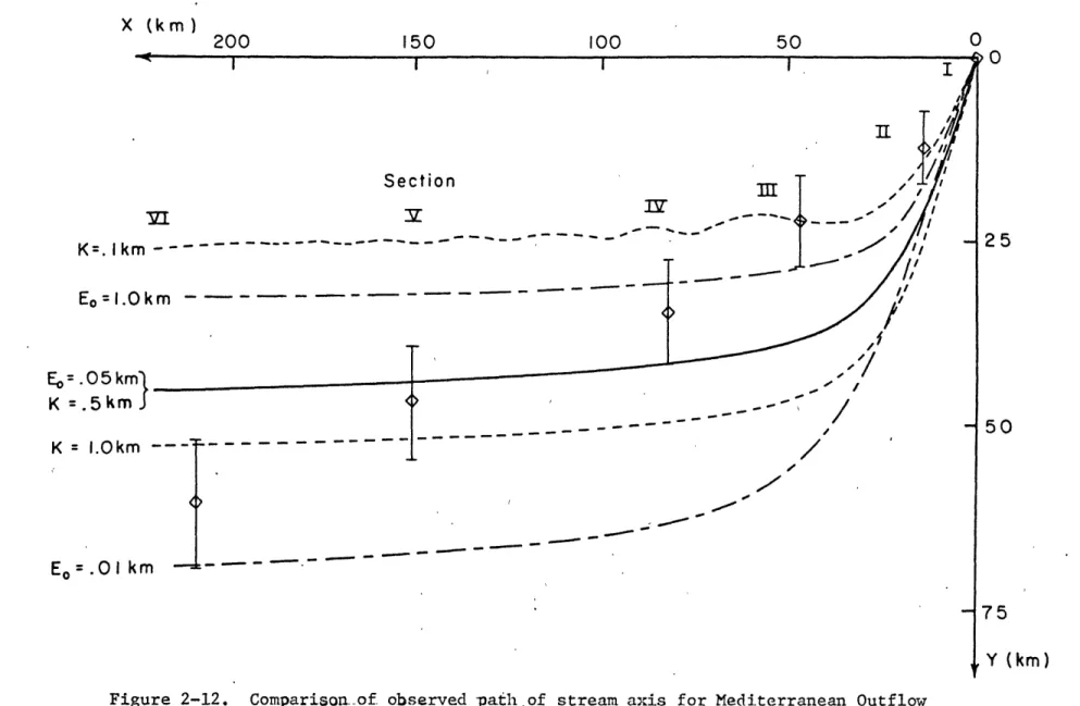
whereas the hydrodynamic stability is weak due to relatively small densi-ty contrasts with the surrounding medium. Evidence for entrainment and mixing of the outflow current with adjacent waters is afforded by water mass analysis of the changing properties at the core of the stream. Moreover, the generally rough topography coupled with high Reynolds numbers suggests that strong turbulence is generated at the base of the flow. The rugged bottom may also exert a strong influence on the path of the outflow current. In the Mediterranean outflow, for instance, the jet which emanates from the Strait of Gibraltar is fragmented into several veins which plunge down submarine canyons as the mean axis of the stream spreads over the northern slope of the Gulf of Cadiz [see Madelain (1969)].
Finally, numerous investigations [Cooper (1955), Mann (1969), Worthington (1969)] have revealed a distinct temporal variability in the overflow currents. However, the details of these fluctuations and their controlling mechanisms are poorly understood, largely because of the difficulty of obtaining adequate synoptic coverage with hydrographic surveys.
Faced with the complexity of these geophysical flows, the theor-etical analysis will be formulated to treat only certain aspects of the fluid dynamical problem. Making use of observed parameters and scales in the outflow data, two separate models which describe steady, two-layer flows over plane topography are presented in the following chapters. In the investigation of.simple dynamical balances, attention will be focused on the effects of entrainment, bottom friction, and
16.
In Chapter II, a streamtube model which describes integral proper-ties of the outflow currents will be formulated and used to determine important scales of motion as well as to demonstrate the gross interac-tion among entrainment, bottom fricinterac-tion, the Coriolis accelerainterac-tion, and stratification of the ambient density field. Empirical laws will be
used in this study to parameterize the entrainment and frictional effects, and the associated proportionality constants are evaluated by comparing solutions of the model equations to hydrographic and current meter data from the Norwegian and Mediterranean outflows. These results provide a consistent overall picture of the outflow dynamics.
In Chapter III, a more detailed Ekman layer model is derived in which entrainment is ignored and the balance between rotation and
fric-tion is examined in a homogeneous environment. The properties of the flow in this model may be related to the distribution of layer thick-ness in the downstream region. However, the general equation governing
the thickness variable is judged to be intractable. Nevertheless, the two important limiting forms of this equation for strong friction and strong rotation may be analyzed and are treated individually in
Chapters IV and V.
A similarity solution for the viscous limit in which weak rotation-al effects are included as perturbations is derived in Chapter IV. The resulting theoretical expressions for the fl6w variables, which are valid over a limited downstream range, are then tested successfully by a series of critical laboratory experiments. In Chapter V, on the other hand, the mathematical analysis of the strong rotation limit leads to a
17.
similarity solution for the thick geostrophic core of the stream. This result is supplemented by a viscous solution valid near the upper edge of the flow. Some exploratory experiments for source flow in a rapidly rotating system will also be described in this chapter.
18.
CHAPTER II
The Streamtube Model
Historically, integral techniques have proved to be very powerful methods in a variety of fluid dynamical applications (e.g. boundary layer theory, hydraulics). In the present context, a streamtube model will be employed to demonstrate some dynamical features of bottom boundary currents. Specifically the effects of entrainment, bottom friction, Coriolis accelera-tion and ambient density stratificaaccelera-tion will be investigated in an attempt to evaluate their relative importance in determining the path of the stream as well as variations in its average flow properties, i.e., mean velocity, density constrast, and cross-sectional area.
The processes of entrainment and bottom friction result from turbulence present in the outflow current which mixes in fluid from the surrounding medium across the upper interface of the flow and transmits momentum to
the bottom by the action of turbulent Reynolds stresses, thereby causing
a drag on the fluid above. To understand fully the physics of these processes, it is essential to distinguish clearly the nature of this turbulence and
the mechanism(s) by which it is generated and maintained. However, for modelling purposes, two different empirical laws will be adopted to account for the effects of entrainment and friction. Each contains an unknown constant which must be determined independently from laboratory experiments or by comparison with observations.
The first of these relations sets the total volumetric entrainment per unit length of the stream equal to a constant fraction of the mean velocity of the flow with a proportionality constant E . A similar
19.
turbulent stratified flow down inclines. Their results indicate that the appropriate value of E for a given physical situation depends rather
0
critically on the "overall Richardson number", Ri0, a stability parameter based on the initial density contrast, characteristic depth, and velocity. On the other hand, the frictional resistance is related to the square of the mean velocity through an unknown factor, K. Quadratic drag laws have been used successfully in a number of oceanographic applications [Defant
(1961)], so estimates of the magnitude of the drag coefficient are avail-able.
In other applications, the coefficients corresponding to E and K are dimensionless. However, in the present context, both E and K are found to have the dimension of length due to an integration performed in the cross-stream direction. Since the analysis only provides information about the area of the cross-stream profile, not its linear dimensions, it is not possible to use average dimensionless coefficients by dividing E and K by the local cross-stream scale. Furthermore, an estimate of the stability parameter is unavailable because the characteristic depth of the layer is unknown. In an attempt to overcome these deficiencies, an al-ternative streamtube model was considered in which the area was expressed as a variable cross-stream dimension times the average layer depth. By analogy to the two-dimensional nonrotating results of Ellison and Turner
(1959), the layer depth was specified to increase linearly in the downstream direction. However, it was felt that the introduction of assumptions about the entrainment process derived from a situation in which the dynamical
20.
could not be justified from a physical standpoint. Moreover, because of the ambiguity involved in assigning particular dimensions to the profiles of actual outflow currents over rough topography, this alternate model was rejected.
The usefulness of the present model lies in its ability to fit observational data with unique values of the empirical constants, E0 and K. Hydrographic sections furnish estimates of the density contrast, cross-sectional area, and path of the stream, while current meter and/or Swallow float data provide estimates of the mean velocity. If all these data can be fit with reasonable accuracy by the solutions for a single parameter pair (E , K), then the dynamical consistency of the model is demonstrated. Once this is achieved, it is then possible, using observed cross-stream dimensions, to estimate average dimensionless friction and entrainment coefficients and compare them to those deduced in other ocean-ographic situations and in laboratory experiments.
21.
II.1 Formulation
A schematic diagram showing the geometrical aspects of the streamtube model is presented in Figure 2-1. The bottom plane is inclined at a small
angle o( to the horizontal, and the rotation-OL and gravity 4. vectors are aligned vertically. Two coordinate systems will be employed in the model. The
first is a Cartesian system whose orientation is fixed by the bottom top-ography. Its origin is located at the source, the x-axis lies along a bottom contour, the y-axis points downslope, and z is measured normal to the bottom.
The second system is a set of streamwise coordinates
({,)
)
in which every point (x,y) in the neighborhood of the current is associated with a normal distance from the stream axis ( 4= 0 ) and a corresponding pointon the axis where f is the distance from the source. The value of
defines uniquely both the position of the axis of the streamtube in the
bottom-fixed coordinates,
(
Xq)
'Y()),
and a local pitch angle, 1
,
between
the streamtube and x axes. Therefore, the equations for the path of the stream are
dXC
-- (2.1)
and - (2.2)
dJ
The governing equations for the streamtube model are derived in Appendix A. The formulation proceeds from the differential equations of motion (rather
than from integral theorems) in order to emphasize the detailed assumptions made in the analysis. The major constraints placed on the mean flow variables
23.
are that the flow is steady, the strong axial velocity and excess density fields are concentrated in a broad, thin layer adjacent to the bottom, and that these quantities are nearly uniform over a cross section of the stream. In addition, the current is narrow in the sense that the cross-stream scale is much smaller than the local radius of curvature of the stream axis. Furthermore, the turbulent velocity and density profiles are assumed to exhibit similarity forms, so that the turbulent stresses and rate of en-trainment may be related solely to the mean velocity and density contrasts
[see Morton (1959)]. The postulated forms for the turbulent entrainment and friction laws are
a) entrainment,
V1
we V
(2.3)
and b) friction,
KY2
+
(T
+
'rl)d(.
dv
1~
(2.4)
where We(_,)
is the entrainment velocity at the interface,
'I~,Q,1)
and are the turbulent stress components (defined in a sense opposing the mean motion) at the bottom and interface respectively, and
are the edges of the flow.
Subject to these conditions, the dynamical equations for the streamtube model have the form
S(AV) =
EW ,
-
(2.5>(AV)
EV
(2.6)A
A COSP3
(2.7)
.. dQ
AY
--
4i )
odi
24.
and
(2.8)
where
\(f)
and A(1) are the mean velocity and density contrasts andA
(1
is the cross-sectional area. In addition to the entrainment constant E and friction coefficient K, the parameters appearing in the equations are the slope , and the normal components of the Coriolis para-meter -=.I
Ceodl
and gravity C6' ( . The excessdensity is defined as the difference between density in the current and the local ambient density, i.e.,
-
)(2.9)ff
where
AA
De
-~o
1
-(2.10)
and
T
=-
T
co-
o( is the stratification rate normal to the plane in the quiescent region. According to the model, the divergence of the downstream volumetric flow rate is measured by the entrainment,E
0V
, thecross-stream balance is geostrophic with a correction for the curvature of the path, , and the divergence of the downstream momentum flux is driven by the downslope component of gravity and retarded by friction.
Considering (2.1) and (2.2) along with (2.5) - (2.10) as the full set of model equations, the mathematical formulation is completed by imposing a suitable set of initial conditions at the source:
25.
A?
A?OI
(2.11)
at
As a further simplification, the Boussinesq approximation is now invoked in the momentum equation which implies
f
except when combined with gravity. After making some convenient definitions,inverse of density contrast, (2.12)
%I
A
Aflux
of excess density,
(2.13)
further manipulation yields the following form for the dynamical equation
(2.14) jA
aN
+
s T r- s
(2.15) es P -- A- , (2.16) and(EOfL
-VVs.
-
(E+4
-'(2.17)
where the initial conditions corresponding to equations (2.14) and 2.15) are
at
0.
(2.18)
14A
FO
A
0A
0
o
Note that the density contrast,
r
, is modified both by entrainment and by the effect of descending along the slope into a denser medium. Also26.
note from equation (2.17) that the entrainment, while not affecting the
momentum flux, has a decelerating effect on the velocity due to the injection of mass into the stream.
Next the variables are normalized in the following way:
r=
~r
6
'
(2.19)
IYO
where the geostrophic velocity scale U and the topographic length scale I, are defined by
A
The full set of dimensionless model equations then takes the form
(2.20)
*jt
H-
(2.21)
(2.22)
and -- (2.23) with ca (2.24)and
dy.
.V
(2.25)
27.
The corresponding initial conditions are
-
=
(2.26)at
1-0.
The dimensionless constants appearing in the equations are the entrainment parameter,
(2.27)
which measures the amount of entrainment over a topographic wavelength, the friction paramter,
(2.28)
which measures the frictional dissipation over that distance, and the stratifi-cation parameter,
2'z (2.29)
which measures the square ratio of the natural frequency for motion along the slope of a particle of density
?
in a stratified syste.m to that in a rotating system.28.
Numerical solutions for the streamtube model were obtained'by integrating equations (2.20) to (2.25) in the downstream direction starting with the
initial values, (2.26). The calculations were performed on an IBM system 360 computer using a modified Adams "predictor-corrector" scheme.
29.
11.2 Approximate Solutions in Limiting Cases
Before proceeding to the comparison with observational data, it is instructive to examine the behavior of solutions to equations (2.20)
-(2.25), subject to (2.26), in several limiting cases. For certain ranges of the parameters ( ' )k ,I ) and in certain regions of the flow,
approximate solutions to this system may be found by asymptotic methods. These solutions fall into two categories:
(i) linearized solutions, which are valid in the vicinity of the source for small values of the parameters and restricted initial conditions, and
(ii) asymptotic solutions in the downstream region
(
- 00 0 ) where irregularities in the flow are damped by friction or entrain-ment and the flow variables attain constant values.In all cases, the results of these approximate analyses are confirmed by quantitative comparison to numerical solutions of the full equations in the appropriate regime.
The most important qualitative features of the streamtube model may be extracted from the case of uniform external density (
i
0).
This limit is characterized by a constant flux of excess density such that14=
go. Therefore, to streamline the notation, it is convenient to define modified entrainment and friction parameters as,- (2.30)
and
(2.31)
30.
Four different limiting cases were analyzed and the resulting approxi-mate solutions are summarized and discussed below. The complete derivation
of these expressions is found in Appendix B.
11.2.1 Small Entrainment and Friction 4 ; Homogeneous
Environment 0 .
For small values of S and )( with
1=-o
, a bilinear perturbation expansion of the dimensionless flow variables yields a linearized solution to streamtube model equations valid in the source region,provided the initial conditions are suitably constrained, i.e.,6 -I-= A . (2.33)
The resulting expressions for the dimensionless variables to first order in
both i and X are
- + (2.34)
0-7) SM'c
~
~
+
A61
Cst
(2.35)
(~-c~
C~
1+
/AT
31.
Note that the presence of the secular terms at first order in % limits the validity of the perturbation scheme to a region { 4
These results indicate that, near the source, a pattern of steady, topographic meanders of wavelength 2TVL arises from mismatches between the imposed initial conditions and the "preferred state":
- I
V
=
1.
Furthermore the appearance of the secular terms at first order implies that initially both the velocity and density con-trast diminish linearly with downstream distance, whereas the area in-creases with ( at twice the rate. The velocity and cross-sectional area both oscillate about these initial trends, while the pitch angle1 oscillates about its preferred value of XC , the friction parameter.
Beyond the region of validity of perturbation theory
(
%
> V),
the numerical solutions indicate that the oscillations induced by the initial conditions are damped and IS approaches a constant value. Furthermore, for large values of the entrainment of friction parameter(
o-C> , I)
the solutions appear critically damped and no'meanders appear.11.2.2 Downstream Limit for Zero Entrainment, =
,
and Homogeneous Environment, t=
0In this asymptotic limit
(
' -' Wo),
the meanders present near the source are damped by friction and the axis approaches a constant pitch angle at which the viscous drag exactly balances the downslope component of gravity. For this case, all flow variables approach con-stant values governed by the following relations32.
Y (2.38)
A
/(2.39)
(2.40)
R
4-_VO
-
(2.41)
The cubic equation for V has only one real root, so choosing its positive square root,
+.'/2'ig + -I4/27-7 (2.42)
serves to specify all the variables uniquely.
In the absence of entrainment and external stratification, the density contrast remains fixed at its initial value. The limiting velo-city exhibits a rather complicated dependence on the friction parameter,
However, for the case of strong friction ( C >
I
)
\r is givenapproximately by,
Vm
~/3
so
UA=
Th
4)
(2.43)
33.
Similarly for the case of weak friction e( 4
so
(2.44)
for
(
.|
In the former case, the velocity is small and the pitch angle approaches a value of , that is, the stream axis points directly downslope. In the latter case, the velocity is near its geostrophic value
(
V/~
I
)
and the pitch angle is very shallow, so the flow tends to follow bottom contours. Notice, the direct dependence of on C in both cases.
11.2.3 Downstream Limit for Zero Friction,
)=
=O
, and Homogeneous Environment, i= 0 .For the frictionless limit
(
( -),
oscillations in the source region decay due to entrainment. As demonstrated in Appendix B, the only constant value of the pitch angle which is consistent with the limiting forms of the equations is/5=0
. Therefore, in this limit, the stream axis ultimately parallels bottom contours.The behavior of the other variables for this case is evident -from their asymptotic forms:
34.
Vas A
-002. (2.46) and
A'
A#('2
'4C
,
(2.47)
The density contrast and velocity decay at a rate proportional to the square root of downstream distance, whereas the cross-sectional area grows linearly with f .
It is possible to extend the results for this limit to include a weak frictional effect if the pitch angle P is assumed to be small but non-zero. The expressions for r' and V' given in (2.45) and (2.46), which are based on the entrainment law and geostrophy, imply a
non-divergent downstream momentum flux. If friction is included for small
P6 , then the remaining balance in the downstream momentum equation yields
ft= -i
'/ ~
(2sg+C)
(2.48)where the value of c is no longer constant but a function of L , i.e.,
c = c( C ). Note that this result is fully compatible with the condi-tion that is vanish downstream. Assuming such a state may be achieved, an estimate of the downstream point beyond which this balance holds is given by
T
(C=6)
(2.49)
I=fT-35.
11.2.4 Small Friction, )III , Weak Stratification,
)
4L.|
Zero Entrainment, S=O .
Significant effects of external stratification can occur only in conjunction with frictional effects since all terms in the model
equa-tions multiplied by t also contain sinf6 which vanishes as t'-P 00
in the absence of friction. However, with friction, the current des-cends the slope into a denser environment, and both the density contrast and the flux of excess density are thereby reduced.
Using an expansion procedure entirely analogous to that used to derive the results for the homogeneous case, with the same constraints on the initial conditions, the perturbation analysis for the case of K
YI<( yields the following expressions for the dimensionless variables:
-
0
+
AV
os 4 +E +Of (2. 50)-)S
VA+
Oc
4+
0 I
(2.51)
S
+j'
f
S'i
4
AcI Cos
+
(2.52)
A
'=
Ao'
i
-(f.-i)
'
+
'
o-
ces')
+
60()
(2.54)Note that the secular terms in these results appear first at order 'tT.,
36.
The pattern of steady meanders which arises in the solution for Z<&GI is preserved here and appears also in the expressions for r' and H' at higher order ( e ). The mean rate of descent, )( , due to frictional influence, is accompanied by diminishing trends in the density contrast and excess density flux which also appear at order . No-tice that despite the expansion of variables in
)C
, the parameter which appears in the final result is the modified friction parameter, )'.The foregoing results will prove useful in interpreting the numer-ical solutions which are to be compared with outflow data.
37.
11.3 Comparison with Norwegian Overflow Data
The observational data to be used for the comparison of the stream-tube model with the Norwegian Overflow come from a series of hydrographic sections taken during cruise BIO 0267 of the C.S.S. Hudson from January to April, 1967 [see Grant (1968)]. Since the purpose of this cruise was
to define the course and water mass characteristics of the outflow, the system of measurement within the current itself was quite comprehensive. An acoustic pinger was attached to the bottom of the wire on all casts
to allow the lowest bottle to be positioned less than 10 meters from the bottom and the bottle spacing was generally 25 meters in the lowest 200 meters of water [see Mann (1969)]. Unfortunately, there are no velocity data available to accompany the hydrographic survey despite
an attempt by Worthington (1969) to measure currents in the Denmark Strait.
The locations of the stations used for this comparison are shown in Figure 2-2. The sections cover the region from the sill of the Den-mark Strait (Section I) to the vicinity of Cape Farewell (Section VII)
along the continental slope of Greenland. Sections I and II were run at the end of January, Sections III and VII in early February, and Sections
IV, V, VI toward the end of March.
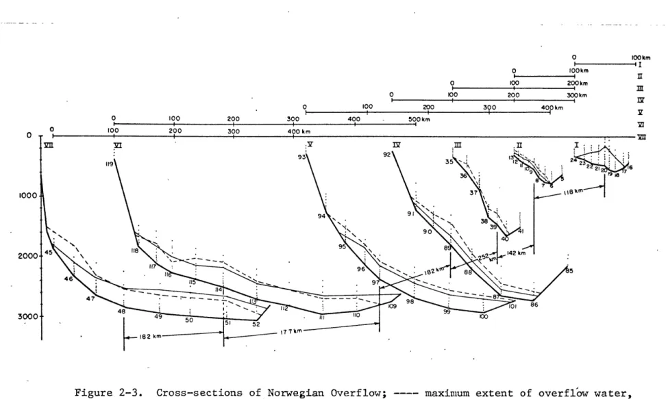
Using smoothed bottom topography, a series of cross-sections of the outflow current showing station locations is presented in Figure 2-3. The overflow water is delineated by two contours. The solid curve is the
G=27.9
contour which according to Worthington (personal com-munication) is a reasonable boundary for the overflow water. The dashed400 350 300 25* 20*
- Figure 2-2. Locations Norwegian Overflow data.
of hydrographic sections for
38.
0 100 200 3 100 200 300 400 500 km 0 200 300 400 km 0 0I
Iv
0 100km 0 100km 100 200km 200 300km 320 40OpkmFigure 2-3. Cross-sections of Norwegian Overflow; ---- maximum extent of overflow water,
40.
curve represents the boundary of maximum vertical extent of the Norwegian Deep Water as determined by a detailed examination of the profiles of
UG , oxygen, and silicates. It is well known that the overflow waters
are characterized by low concentrations of nutrients, especially reactive silicates, high oxygens, and, of course, large densities [Stefansson
(1968)]. Typically, the profiles of potential density and the chemical tracers show a marked variation at some point near the bottom, below which these properties are relatively uniform (see Figure 2-4). The vertical extent of the outflow is defined by the top of this gradient, where the oxygen and silicates, in particular, take on values character-istic of the local environment. The potential temperature-salinity diagrams for these stations indicate that these contours contain pure Norwegian sea water which has been degraded by mixing with the Atlantic water, the East Greenland Current and water derived from the
Iceland-Scotland overflow [Mann (1969)]. Figure 2-3 also -illustrates one of the fundamental difficulties in fashioning a steady model after obser-vational data, namely the absence of TG=27-9 water at Section III. According to Mann (1969), this observed variability in composition may be ascribed to the fact that waters from different depths in the Nor-wegian Sea flow over the sill at different times. This conclusion is
supported by other observations of radical changes in the thickness of the overflow layer in the Denmark Strait over a period of hours [Harvey
(1961)]. However, in terms of the stream dynamics, it is significant that a small but distinct density contrast and trace elemnt anomalies are evident along the slope at this section, indicating that a weak flow still exists. Furthermore, except for this section, the continuity
SECTION II Station 12 SECTION V Station 97 SECTION VU Station 47 02
ogSiO
3 ~ I I - (--0-8 ( O 3 gm/cm 3 ) 02 ( m 1 /1 ) SiO 3 (p1 g at/j) 27.5 6.6 5 27.7 6.8 7 z -500m 02 -400 -300 0'8'-N
-200 i0O~ --- i ' / 27.9 7.0 9 7-/ / 28.1 7.2 27. 5 6.5 5, 27.7 6.7 7Figure 2-4. Profiles of potent.ial. density. for typical stations in the Norwegian overflow.
z -500m
.SiO
3 400 300 200 -100\ 27.9 28.1 6.9 7.1(7)
27.5 6.4 6 02 / ~1'z
-8 50 4 3C -12 10 0m 00 0 00 0~
27.7 27.9 28.1 6.6 6.8 7.0 8 0 2, oxygen, and silicates
SiO
342.
of average flow properties does not seem to be broken. Therefore, it may be argued that the drastic departure of Section III from the overall pattern results from an isolated cutoff of Norwegian Deep Water at the sill and that further evidence of temporal variability of the source
conditions or the flow itself remains at or below the noise level of the measurements. Hence, data from Section III is incompatible with data
from other sections and will not be considered in the following compar-ison. Explicitly, it is assumed that the break in flow pattern at this point represents a local disturbance which propagates along the stream
exerting a relatively minor effect on the average flow properties in other segments of the stream or on the overall dynamical characteristics
such as the path of the stream.
In order to produce a meaningful comparison with theory, the physi-cal constants appearing in the model equations as well as the average flow properties must be extracted from the hydrographic data in a way
that is consistent with the premises on which the model is based. First of all, the bottom slope, S =
t0V%
L , was computed by fitting astraight line across each section through the observed depths of all stations at which overflow water was present. The mean slope was then obtained by averaging over all sections. Secondly, the mean Coriolis parameter was taken to be twice the value of the vertical component of
the Earth's rotation near the center of the outflow current at a lati-tude of 64* N. Also the stratification of the ambient fluid was deter-mined by fitting a straight line to the density field adjacent to the overflow water at several typical downstream stations. This procedure
43.
rate, T, and corresponding stratification parameter, 't . Finally,
standard values were adopted for the gravitational acceleration, =
and characteristic density,
j'
. These physical properties of the system are compiled in Table I.The measureable average flow properties are the density contrast, Af the cross-sectional area, A, and the pitch angle,
3
. Using the profiles of G0 , oxygen and silicates and the temperature-salinity diagram to dis-tinguish the transition between overflow and adjacent waters, the density contrast at each station was determined as the maximum difference in potential density across the interface, i.e., between the density at the top of the strong gradient in properties and the maximum interior value. The station values were then averaged over each section to obtain a sectional mean density contrast. However, in most cases it was found that these average valueswere severely degraded by the small differences observed at stations near
the edges of the flow and that the estimates were, therefore, not truely representative. To counterbalance this effect, the value of. A used for the comparison with the streamtube model is the average between the density contrast at the core station (maximum
Ai
) and the sectional mean value. This procedure tended to weight the relatively uniform values at and about the core station more heavily in the estimate. An attempt was also made to refine the values of At at each station by integrating graphically the area between the observed density profile and the extrapolated ambient density profile and then dividing by the thickness of the overflow layer to obtain a true vertically-averaged density contrast. The results derived by this technique for stations near the axis of the flow agreed quite well with the44. TABLE I. Physical Constants, Initial Conditions and Scales for the
Norwegian Overflow Comparison
Quantity
Bottom Slope Coriolis Parameter Ambient Stratifi-cation Rate Dimensionless Stratification Parameter Characteristic Density Gravitational Acceleration Initial Density Contrast Initial Value of Cross-sectional AreaInitial Pitch Angle Initial Velocity Geostrophic Velocity Scale Topographic Length Scale Symnbol s = tan a f = 2Q cos a T = T cos a 2g y = s 2 _ f p0 g = g cos a Ap 0 A 0 V 0 sgAp U 0 L = U/f Value + Error (.58 + .26) x 10-2 -4 (1.30 + .04) x 10. /sec (.66 + .09) x 10 9/cm (1.29 + .18) x 103 1.00 gm/cm3 980. cm/sec2 -3 3 .38 x 10 gm/cm 7.84 km2 .112 16.0 cm/sec 16.6 cm/sec 1.28 km
45.
sectional mean values; however, these estimates were very sensitive to the layer thickness chosen and varied radically near the edges of the flow where there was little excess density. This method was, therefore, rejected because of its inability to produce stable estimates of average contrasts of the cross section. In summary, the density contrast used in the streamtube model
comparison was computed by averaging the potential density difference observed at the core station (maximum value) with the sectional mean of those differ-ences. This method is simple and relatively unambiguous and leads to stable values of the average density contrast for each section.
The area of the stream cross section was computed by graphically inte-grating the area between the dashed curve and the smoothed bottom contour. in Figure 2-3. By this technique irregularities in the true bottom topography were neglected and the cross-stream profile encompasses all of the water whose origin could be traced to the Norwegian Sea. Furthermore, at each section the axis of the stream was assumed to pass through the core station where the maximum density contrast was observed. In most cases, this point nearly coincided with an alternate criterion, the centroid of the cross-sectional area, and differences between the two could be used as a measure of the error
involved in the estimate. Once the path of the axis was determined, the average pitch angle between sections could be measured.
When the hydrographic data had been reduced-to the appropriate set of average flow properties, the initial conditions were selected and the numeri-cal solutions to equations (2.20) to (2.25) were computed. Due to the distor-tion of the outflow profile at Secdistor-tion I by the presence of the East Greenland Current, the flow properties at Section II were adopted as initial conditions. In fact, the integration may be started at any point in the stream since t
46.
does not appear explicitly in the equations. Furthermore, since there were no velocity data available, the initial velocity was assumed to be in geo-strophic balance, i.e.,
Ce t
(2.55)
The initial pitch angle, (A , was derived from the path of the stream between Sections I and II. The values of all the initial conditions plus the corres-ponding velocity and length scales are tabulated in Table I.
Starting with estimates of the empirical constants (E , K) obtained by matching initial trends in the data with approximate solutions for the case a , optimum values for E and K were sought by trial and -error. The numerical solutions are compared to the average flow properties derived from the hydrographic data in Figures 2-5 to 2-7. It is found that all the observations can be adequately fit with a unique pair of empirical constants,
(E-
io
O
-(2.56)
Furthermore, all the data points may be encompassed by varying these optimum values by less than a factor of two.
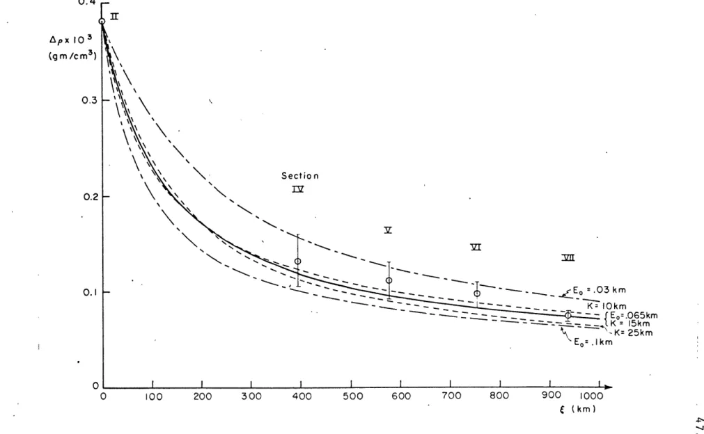
Figure 2-5 shows a comparison of the average density contrasts. As expected, & is found to be a strong function of the entrainment rate, but depends weakly on the magnitude of the. friction coefficient. The error bars on the data points represent the difference between the density contrast observed at the flow axis and the sectional mean value. Next, the path of
0.4
Ap
x10
3 (g m /c m3) 0.3 0.2-0.1 -0L
0 100 Section - - - - =.03 km K= 25km 200 300 400 500 600 700 800 900 1000 ( (km)Figure 2-5. Comparison of average density contrant in Norwegian Overflow data
48.
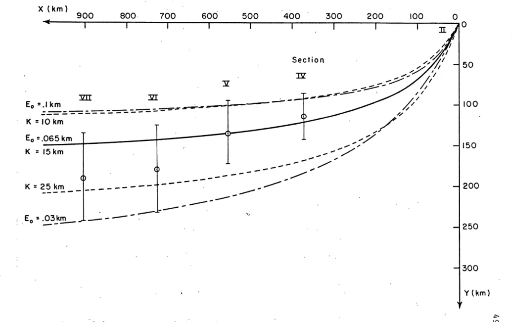
the stream is plotted in bottom-fixed coordinates in Figure 2-6. The coordin-ates (
X,Y
) of the observed stream axis were computed from geometrical relations using the depth of the core station and the mean bottom slope. This calculation implicitly involves the mean pitch angles between sections. The error bars on the data points reflect the uncertainty in the axis position as measured by the distance between the core station and area centroid at each cross section. The trajectory of the stream axis is controlled strongly by both the friction and entrainment constants. In Figure 2-7, the rate of increase of cross-sectional area is seen to depend heavily on the entrainment rate, but weakly on the strength of friction. The error bars attached to the observational points represent uncertainty in the area measurements as determined from the difference in the areas under the solid and dashed curves in Figure 2-3.Lastly, for the sake of completeness, the theoretical mean velocity distribution along the stream is presented in Figure 2-8. The locations of Sections IV to VII are also indicated. According to this prediction, the average current drops very rapidly near the source from its initial value,
V=
I=o.
*/Sec , to a value of 10.8 cm/sec just 10 km. downstream, thendiminishes gradually to a value of 3.26 cm/sec at Section VII. Combining this information with the cross-sectional area results indicates that the volumetric flow rate of the outflow current,
=
AV
(2.57)6 3
has increased from a value of 1.3 x 10 m /sec at the source to roughly 6 3
4.6 x 10 m /sec at Section VII. In his water budget for the Norwegian Sea, Worthington (1970) used estimates obtained from dynamic computations
X (km)
900
800-
700
600
500
400
300
200
100
0
Section
E.
=.I
km
K
= 10 kmEO
=.065
km
K
=
15 km
K= 25 km
E
=.03km
I
-- - --7
- - -. .... -- --Figure 2-6. Comparison of observed path of stream axis for Norwegian Overflow
with streamtube axis for several parameter pairs (E0,K).
0
50
100
150
200
250
300
Y (km)
E0=.km / Section 10 -I-E =.065km 2K= 15km K=25km7 -. deK=10km E= -. 03 km I I 200 300 400 500 600 700 800 900 1000 (km) Figure 2-7. Comparison of cross-sectional area. variationfor.Norwegian.
Overflow data with streamtube model results for several parameter pairs (E ,K).
A (km 2 ) 120 100 80 60 40 20
-/
-I 10016.0 -r JI 14.0 V (cm /sec) 12.0 10.0 8.0 6.0 4.0 2.0 0 Section
NI
j
MEI K =10 km K = 2 5 k m - E=.030km Eo=.10km 0 100 200 300 400 500 600 700 800 900 1000(
(km)52.
and neutrally buoyant float measurements to arrive at transport values of
6 3 6 3
4 x 10 m /sec for the Denmark Strait overflow and 10 x 10 m /sec for the total transport southwest of Greenland. Each of Worthington's values ex-ceeds the corresponding value here but the ratios of the two, i.e., the factors by which the transport is enhanced due to entrainment, are roughly comparable. Moreover, in a separate computation designed to match a transport value of 4 x 10 m /sec at the source
( e
= ' = 51 cm/sec), the6 3
transport grew to a value of 9.3 x 10 m /sec at Section VII using the same optimum pair of coefficients (E , K). This fact is further evidence of the consistency of this model with observational data.
The numerical solutions may be interpreted with knowledge of the values of the modified entrainment and friction parameters,
-1 .(2.58)
and
YC =z54 (2.59)
which correspond to the optimum values of the empirical constants, (E , K) =
(.065, 15) km. First of all, the strong frictional influence indicated by the value of X accounts for the absence of oscillations in the flow proper-ties and stream path near the source. Instead, the velocity and
cross-sectional area change rapidly from their initial values to levels appropriate to the non-entraining downstream limit
53-The initial pitch angle likewise adjusts to its limiting value,
/3=
.94-.
The density contrast, on the other hand, is invariant in the non-entraining limit. It, therefore, undergoes no drastic changes in the source region but varies smoothly over the entire length of the stream. The sharpest decrease in
A
f
occurs within a distance of 100 or 200 km. from the source, which corresponds generally to an entrainment length scale introduced in(2.34), namely *= =
104.
km.The character of the downstream variations of A , , , and A, and their dependence on the value of E0, suggest the asymptotic behavior of the stream is controlled by the entrainment with a weak frictional influence. In fact, quantitative comparison of the linear variation in cross-sectional area reveals that the slope of the numerical solution (.15 km 2/km) between Sections V and VI differs from that in the limiting case,
'a.
Moreover, the inverse square root dependences of Af and
Y
do not hold exactly and the trend in/3
is different from that .predicted by (2.48).A
However, a special computation for the case of T = 0 reveals that these dis-crepancies can be fully accounted for by the presence of a weak ambient strati-fication. It may be concluded, therefore, that the behavior of the solutions in the downstream region is strongly controlled by the entrainment parameter,
The transition to this state appears to occur somewhat before tT = 500 km., which is predicted by equation (2.49) for P = 0.1.
54.
The pronounced influence of the strength of friction on the path of the stream axis is anticipated from the direct dependence of the pitch angle on
)C
for all limiting cases in which it is non-zero. The dependence on E , however, is related to the damping of the flow by entrainment and may be explained qualitatively by reference to (2.49). For fixed)-ce
"
,strong entrainment (large 5 ) helps damp the velocity and causes a rapid transition to the asymptotic state of flow along bottom contours. If the entrainment is weak, however, the transition is delayed, thereby allowing the axis a larger excursion downslope.
Finally, with regard to the effects of ambient stratification, the
A
results of the computation for T = 0 mentioned above showed relatively minor differences (not exceeding 25%) in the flow properties at Section VII from those corresponding to the stratified case,accompanied by a slight shift of the stream axis downslope.