Toronto-area ozone: Long-term measurements and modelled sources of poor air quality events

HAL Id: insu-01236182

https://hal-insu.archives-ouvertes.fr/insu-01236182

Submitted on 31 Aug 2020

HAL is a multi-disciplinary open access

archive for the deposit and dissemination of

sci-entific research documents, whether they are

pub-lished or not. The documents may come from

teaching and research institutions in France or

abroad, or from public or private research centers.

L’archive ouverte pluridisciplinaire HAL, est

destinée au dépôt et à la diffusion de documents

scientifiques de niveau recherche, publiés ou non,

émanant des établissements d’enseignement et de

recherche français ou étrangers, des laboratoires

publics ou privés.

Cynthia H. Whaley, K. Strong, D. B. A. Jones, T. W. Walker, Z. Jiang, D. K.

Henze, M. A. Cooke, C. A. Mclinden, R. L. Mittermeier, Matthieu Pommier,

et al.

To cite this version:

Cynthia H. Whaley, K. Strong, D. B. A. Jones, T. W. Walker, Z. Jiang, et al..

Toronto-area

ozone: Long-term measurements and modelled sources of poor air quality events. Journal of

Geo-physical Research: Atmospheres, American GeoGeo-physical Union, 2015, 120 (21), pp.11368-11390.

�10.1002/2014JD022984�. �insu-01236182�

Toronto area ozone: Long-term measurements and modeled

sources of poor air quality events

C. H. Whaley1_{, K. Strong}1_{, D. B. A. Jones}1_{, T. W. Walker}1_{, Z. Jiang}2_{, D. K. Henze}3_{, M. A. Cooke}1_,

C. A. McLinden4_{, R. L. Mittermeier}4_{,M. Pommier}5_{, and P. F. Fogal}1

1_{Department of Physics, University of Toronto, Toronto, Ontario, Canada,}2_{Jet Propulsion Laboratory, California Institute of}

Technology, Pasadena, California, USA,3Department of Mechanical Engineering, University of Colorado Boulder, Boulder, Colorado, USA,4_{Air Quality Research Division, Atmospheric Science Directorate, Science and Technology Branch,}

Environment Canada, Toronto, Ontario, Canada,5_{Sorbonne Universités, UPMC Univ. Paris 06, Université Versailles}

St-Quentin, CNRS/INSU, LATMOS-IPSL, Paris, France

Abstract

The University of Toronto Atmospheric Observatory and Environment Canada’s Centre for Atmospheric Research Experiments each has over a decade of ground-based Fourier transform infrared (FTIR) spectroscopy measurements in southern Ontario. We present the Toronto area FTIR time series from 2002 to 2013 of two tropospheric trace gases—ozone and carbon monoxide—along with surface in situ measurements taken by government monitoring programs. We interpret their variability with the GEOS-Chem chemical transport model and determine the atmospheric conditions that cause pollution events in the time series. Our analysis includes a regionally tagged O₃model of the 2004–2007 time period, which quantifies the geographical contributions to Toronto area O3. The important emission types for 15

pollution events are then determined with a high-resolution adjoint model. Toronto O3, during pollution

events, is most sensitive to southern Ontario and U.S. fossil fuel NOxemissions and natural isoprene emissions. The sources of Toronto pollution events are found to be highly variable, and this is demonstrated in four case studies representing local, short-, middle-, and long-range transport scenarios. This suggests that continental-scale emission reductions could improve air quality in the Toronto region. We also find that abnormally high temperatures and high-pressure systems are common to all pollution events studied, suggesting that climate change may impact Toronto O3. Finally, we quantitatively compare the sensitivity

of the surface and column measurements to anthropogenic NOxemissions and show that they are remarkably similar. This work thus demonstrates the usefulness of FTIR measurements in an urban area to assess air quality.

1. Introduction

In Canada, ground-level ozone (O3) is one of five pollutants that are monitored regularly and deemed a health

risk. The four others are fine-mode particulate matter (PM2.5), nitrogen oxides NO and NO2(= NOx), and carbon monoxide (CO). Overall, air quality in Canada has improved over the last few decades. There is a human health standard for the surface concentration of each pollutant, and in Ontario, the standards for NO_xand CO have not been exceeded in over 20 years [MOE, 2012]. Even the standard for PM2.5 has not been exceeded in Ontario since 2008 [MOE, 2013]. Only O3continues to exceed standards in most parts of Ontario every summer

[MOE, 2013].

In Ontario, there are two standards of surface O3concentration for human health: the provincial 1 h criterion,

which is 80 ppb and the Canada-Wide Standard (CWS) 8 h running average criterion, which is 65 ppb (although the latter is being replaced with the Canada Ambient Air Quality Standard, of 63 ppb 8 h average in 2015). From 2002 to 2010, Toronto averaged 8 days per year that exceeded the 1 h criterion for surface O₃and 18 days per year that exceeded the CWS.

The relationship between O3and its precursors is not linear [Sillman, 1995], and this is what makes it so

diffi-cult to control. Over most of North America, O₃is in a NO_x-limited regime, in which O₃production is linearly proportional to NOxconcentrations. However, when NOxconcentrations are very high, O3production

tran-sitions to a hydrocarbon-limited regime, in which production of O3is linearly proportional to hydrocarbon

RESEARCH ARTICLE

10.1002/2014JD022984

Key Points:

• Eleven years of Toronto tropospheric O₃and CO measured at surface and with FTIR

• Modeling quantifies key geographical sources and emissions for Toronto O3

• NO_xemissions from southern Ontario and northeast U.S. cause pollution events

Supporting Information:

• Texts S1 and S2 and Figures S1–S4

Correspondence to:

C. H. Whaley,

[email protected]

Citation:

Whaley, C. H., et al. (2015), Toronto area ozone: Long-term measurements and modeled sources of poor air quality events, J. Geophys. Res.

Atmos., 120, 11,368–11,390,

doi:10.1002/2014JD022984.

Received 18 DEC 2014 Accepted 13 OCT 2015

Accepted article online 17 OCT 2015 Published online 10 NOV 2015

©2015. American Geophysical Union. All Rights Reserved.

concentrations and inversely proportional to NOxconcentrations [e.g., Kleinman et al., 2000; 2005; Sillman and

West, 2009; Parish et al., 2011; Jing et al., 2014; Zhang et al., 2014].

O3pollution events in southern Ontario and the northeastern U.S. are typically associated with the

devel-opment of high-pressure systems in central Canada. These systems can either move southeastward into the midwestern U.S. or eastward across the Great Lakes and over Toronto [Zishka and Smith, 1980; Yap et al., 2005]. Additionally, Zhu and Liang [2012] have shown that the westward extent of the Bermuda High has a large effect on air quality in the northeastern U.S. (and by extension, southern Ontario). When the Bermuda High is extended to the west, the air circulating clockwise on its western side brings clean ocean air to the south-eastern U.S., but by the time it reaches the northsouth-eastern U.S. it has accumulated a large amount of isoprene (a volatile organic compound, VOC) and anthropogenic pollutants, which create O₃.

A study of Toronto’s surface O₃in the summer of 1998, on O₃exceedance days, attributed only 9% of the O₃to Ontario emissions and the rest to transboundary transport of pollutants [Yap et al., 2005]. Southern Ontario is downwind of major U.S. pollution sources, such as the Ohio valley. Fortunately, in the U.S., air quality policies such as the Clean Air Act, the Environmental Protection Agency (EPA)’s State Implementation Plan (known as the “NO_xSIP Call” program, which was a NO_xemissions trading program among 22 eastern states from 2003 to 2008), the Clean Air Interstate Rule, and the Tier 2 Light Duty Vehicle Emission Standards [EPA, 2012] have caused NOxemissions to be reduced by industries and transportation at a rate of about 2–3%/yr [Gilliland et al., 2008; Godowitch et al., 2010; EPA, 2012; Zhou et al., 2013]. In Canada, air quality policies, such as the Industry Emission Reduction Program (also a cap and trade NO_xprogram), the phase out of coal power plants in Ontario, and Ontario’s Drive Clean Program [Yap et al., 2005] have caused NO_xemission reductions in Ontario at a rate of 3.6%/yr [MOE, 2013]. There was also the Canada-U.S. Air Quality Agreement in 1991 that was initially intended to address acid rain but was amended to include an Ozone Annex in 2000 [Yap et al., 2005]. The result is that the number of high O₃days has been dramatically reduced in both the eastern U.S. and Canada.

That said, air quality remains an issue. Mean surface O3in Toronto increased by 4.2%/yr from 1991 to 2011

[MOE, 2013], and air quality is expected to get worse with climate change [Leibensperger et al., 2008; Jacob

and Winner, 2009; Millstein and Harley, 2009; Turner et al., 2013]. Not only will global warming increase surface

temperatures but it is also expected to reduce the number of cyclones (low-pressure systems) that remove O3

air pollution and shift the cyclones poleward [Leibensperger et al., 2008; Turner et al., 2013]. Also, transbound-ary transport of O₃and its precursors caused by hemispheric anthropogenic emissions of NO_xand VOCs is increasing, thus resulting in higher background O3[Fiore et al., 2002; Oltmans et al., 2006; Zhang et al., 2011].

Therefore, the continued monitoring of tropospheric O₃over populated areas is important. In addition to in situ O3measurements from the National Air Pollution Surveillance Program (NAPS) in downtown Toronto, at

the University of Toronto Atmospheric Observatory (TAO), lower tropospheric (0–5 km) O3columns (hereafter,

“lower tropospheric columns”) have been measured for over a decade with a ground-based, high spectral res-olution Fourier transform infrared (FTIR) spectrometer. The primary goal of this work is to examine how the lower tropospheric O3and CO column measurements from TAO can be used to assess air quality, with a focus

on determining the factors affecting tropospheric O3in Toronto. However, as this is the first time the FTIR

data set has been shown, the second goal of this work is to describe the measurements and then use them to characterize Toronto area lower tropospheric O₃. The promise of using ground-based FTIR measurements for this purpose has been shown for O3in Viatte et al. [2011] and for CO and NO2in Lindenmaier et al. [2014]. The

GEOS-Chem chemical transport model (CTM) is employed to interpret the data, but first we show how well it performs at reproducing Toronto area O3and CO. We then determine the causes of the short-term

enhance-ments seen in the time series during the spring, summer, and fall months. Using the GEOS-Chem tagged O₃ forward model and the sensitivity adjoint model, we aim to answer the question: What are the important causes of Toronto regional O3pollution, in terms of geographical regions, emission types, and processes?

The measurements are described in section 2, and the GEOS-Chem simulations are described in section 3. Section 4 presents 11 years of measurements and the model time series, and section 5 highlights and discusses 15 pollution events between 2004 and 2007, along with their dominant geographical sources from the tagged model. The sensitivity of O₃to precursor emissions is explored for these pollution events in section 6. Finally, in section 7, we summarize our findings for causes of enhanced Toronto O₃pollution, and we justify the use of the lower tropospheric column measurements for air quality studies.

Table 1. TAO and CARE FTIR Retrieval Parameters: Spectral Fitting Microwindows, Fitted Interfering Species, Measurement SNR From Tradeoff Curve, Diagonal Elements of the A Priori Covariance Matrix (S_a), Median DOFS (Over 11 Years) for Total and Lower Tropospheric Columns, and Errors (Total/Random) on the Lower Tropospheric Columns of O₃and CO

Species O₃ CO

NDACC filter 6 (HgCdTe detector) 4 (InSb detector)

Microwindow(s) (cm−1_{) 1000.00–1005.00 2057.70–2058.00} 2069.56–2069.76 2157.50–2159.15 Interfering species H₂O, CO₂, CH₄, O₃isotopes O₃, CO₂, OCS

O₃, CO₂, OCS O₃, CO₂, OCS, N₂O, H₂O

SNR 35 100

S_a 20% 20–30%

DOFS 4.8/1.0 2.5/1.1

Lower tropospheric column errors 19%/5.7% 4.6%/0.9%

2. Measurements

2.1. TAO FTIR Spectrometer

The primary measurements used in this study are made by a ground-based, high-resolution (0.004 cm−1₎

Bomem DA8 FTIR spectrometer at TAO (43.66∘N, 79.4∘W, 174 m asl; above sea level) [Wiacek et al., 2007]. The TAO FTIR spectrometer was installed in late 2001 and has been operational for daily measurements, weather permitting, since May 2002. TAO became a site in the Network for Detection of Atmospheric Composition Change (NDACC) in 2004. We retrieve total and partial column amounts of O3 and CO

using the optimal estimation method [Rodgers, 2000] implemented with the SFIT2 [Rinsland et al., 1998;

Pougatchev et al., 1995] v3.94 algorithm, and the High-resolution Transmission molecular absorption database

2008 spectral line list [Rothman et al., 2009]. Temperature and pressure profiles are obtained from the National Centers for Environmental Prediction Climate Prediction Center meteorological data product (hyperion.gsfc.nasa.gov/Data_services/automailer/index.html) for z = 0–50 km, and the mean of a 40 year run (1980–2020) of the Whole Atmosphere Chemistry Climate Model (WACCM, version 6, Eyring et al. [2007]) for Toronto (J. Hannigan, NCAR, personal communication, 2009) for z = 50–120 km.

The retrieval parameters at TAO were recently updated [Whaley et al., 2013]; the a priori volume mixing ratio (VMR) profiles now come from the mean of the same 40 year WACCM run mentioned above. The spectral microwindows have been updated to those recommended by the NDACC-Infrared Working Group (IRWG) harmonization initiative (which seeks to have all NDACC-IRWG sites use the same retrieval parameters for consistency, www.acd.ucar.edu/irwg/).

The O₃and CO microwindows fall in the spectral range of different NDACC FTIR filters (6 and 4, respectively) and are thus measured at slightly different times. Also, the O₃retrievals are obtained from spectra measured with a different detector than is used for CO. There are about half as many O₃measurements as CO measure-ments from 2002 to 2013 due to technical problems with the detector used for O₃; however, since 2010 this has not been an issue.

Table 1 lists the retrieval parameters used and the resulting median degrees of freedom for signal (DOFS, defined as the trace of the averaging kernel matrix [Rodgers, 2000]) for the total columns and the lower tro-pospheric columns, over the 11 year data set. Table 1 also lists the total errors on the lower trotro-pospheric columns and the random component of the errors (discussed below). The signal-to-noise ratios of the mea-surements (SNR, related to the diagonal elements of the error covariance matrix, S_e, with no off-diagonal elements [Wiacek et al., 2007]) were chosen based on a root-mean-square fitting residual versus SNR tradeoff curve for each species [Batchelor et al., 2009]. The a priori covariance matrix (S_a, diagonal elements of corre-sponding standard deviations listed in Table 1) for O3was chosen based on the variance seen in its Halogen

Occultation Experiment measurements over Toronto and for CO was chosen based on the variance seen in its GEOS-Chem model simulation [Wiacek et al., 2007]. We use a Gaussian correlation length of 4 km for off-diagonal elements of Sa[Wiacek, 2006; Wiacek et al., 2007].

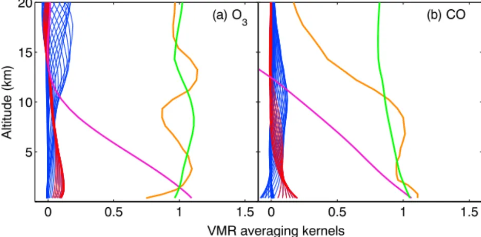
Figure 1. TAO VMR averaging kernels (blue lines, with those for the 0–5 km levels in red lines), total column averaging kernels (green lines), partial (0–5 km) column averaging kernels (purple lines), and sensitivity (orange lines) for: (a) O₃ and (b) CO.

The lower tropospheric columns (defined as 0–5 km in this study) of O3and CO have total errors of 19% and

4.6%, respectively. These are total error budgets that include spectroscopic errors (line width and line intensity, which together are the dominant sources of error), measurement, smoothing, temperature, interference, and solar zenith angle errors, calculated as described in Batchelor et al. [2009] and Lindenmaier et al. [2010]. When only random errors (eliminating spectroscopic errors, which are systematic) are taken into account (i.e., when discussing changes within the time series), the errors are 5.7% and 0.9% for O3and CO, respectively. These are

summarized in Table 1.

Because FTIR solar absorption measurements can only be made when skies are clear, at TAO we typically have 80 to 100 days of measurements per year, with greater coverage in the summertime and a greater number of measurement days in recent years due to improvements in efficiency and instrument maintenance. However, this sampling limitation does not impact the conclusions of this study, which is focused mainly on summer-time, daytime O₃. Also, note that each TAO measurement is recorded over approximately 20 min (except for measurements starting in 2014 which are recorded over approximately 10 min).

The TAO averaging kernels characterize the vertical information contained in the FTIR retrievals [Rodgers, 2000]. Figure 1 shows typical TAO VMR averaging kernels for total column O₃and CO retrievals along with the lower tropospheric column averaging kernels, which are equal to the VMR averaging kernels weighted by the density, summed over the layers of interest. Also plotted is the sensitivity, Sk, at each altitude, k (equation (1))

Vigouroux et al. [2008]:

Sk= ∑

i

Aki, (1)

where A is the averaging kernel matrix, and the summation is over the i elements of the kth row. When the sensitivity is above 0.5, it means that the measurements are contributing more than 50% to the retrieved profile (with the rest coming from the a priori profile). The O₃and CO retrievals have excellent sensitivity (S_k ∼ 1) in the troposphere. The peak of the O₃sensitivity is around 2 km in altitude, which means that the lower tropospheric columns will be sensitive to long-range transport of O3and its precursors. About 80% of

the lower tropospheric columns (0–5 km) comes from 0–4 km (1000–550 hPa) and 0–3 km (1000–650 hPa) for O₃and CO, respectively.

2.2. CARE FTIR Spectrometer

Environment Canada’s Centre for Atmospheric Research Experiments (CARE) is located at Egbert, Ontario, about 80 km north northwest of Toronto at 44.23∘N, 79.78∘W, 251 m asl. Measurements with a Bomem DA8 FTIR spectrometer began at CARE in January 1996, although we only examine the data set from 2002 onward when we have complementary TAO data. Egbert is relatively close to Toronto, yet it is located in a rural area. Pollution measured at Egbert likely undergoes the same long-range transport as that measured in Toronto, but has fewer local sources, except possibly additional agricultural sources.

The frequency of Egbert measurements varies greatly from year to year due to the availability of staff and instrument downtime for maintenance, repair, and upgrades. The greatest number of measurement days (about 30 per year) occurred during 2002–2007, and there were very few in 2008–2010, and none in 2011–2013.

The CARE time series were retrieved using the same parameters as for TAO (Table 1), and the averaging kernels are very similar to those in Figure 1.

Comparisons between same-day CARE and TAO lower tropospheric O3 and CO columns were made

(of which there were 52 overlapping measurement days), and mean differences of 3.9% and 13.2% (TAO-CARE/TAO × 100%), respectively, were found over the full time series. Given the random errors on the lower tropospheric columns (both CARE and TAO use the same spectroscopy, so systematic errors can be ignored), the difference in O₃lower tropospheric columns between the two sites is not significant, despite more CO and NOxemissions in Toronto than in Egbert. This is likely due to the free tropospheric component, in which both Toronto and Egbert would have similar composition, given their proximity. For example, winds above 3 km are typically 12.6 m/s (taken from the median of the GEOS-5 wind fields over Toronto), so it would only take about 1.8 h to travel from one place to the other, which is shorter than the lifetime of O3in the free

troposphere. For CO, the large difference is likely because of the boundary layer component, where CO con-centrations and the FTIR averaging kernels peak and for which Toronto is expected to have more CO than Egbert, due to anthropogenic emissions.

For the rest of this study, we treat the CARE O3lower tropospheric columns as a complementary data set that

helps fill in the gaps of the TAO data set (which adds 150 additional measurement days). For CO, we include the CARE lower tropospheric columns; however, we keep in mind the difference between the two sites in our analysis of pollution events.

2.3. Satellite Observations: TES and MOPITT

In order to supplement the TAO FTIR measurements of tropospheric O3and CO, we use lower tropospheric

column measurements from the Tropospheric Emission Spectrometer (TES) and the Measurements of Pol-lution in the Troposphere (MOPITT) satellite instruments when they pass over the Toronto area within ±1∘ latitude and longitude. This spatial coincidence criterion was selected to approximate the same area as the GEOS-Chem 2∘ × 2.5∘ grid box that includes both the Toronto and Egbert measurement locations. These instruments and their data sets, including their comparison to TAO measurements are described in the supporting information.

2.4. Surface In Situ Measurements

The Environmental Monitoring and Reporting Branch of the Ontario Ministry of the Environment (MOE) oper-ates 40 ambient surface air monitoring sites across Ontario, as part of the NAPS program. Each site measures a number of pollutants hourly. There are four sites in the Toronto region: Toronto West, Toronto North, Toronto East, and Downtown Toronto. The Downtown Toronto site (located at Bay Street and Wellesley Street W., site ID 31103) is the most densely populated of these sites and only 1 km from TAO, so its O3, CO and NOx measurements are used in this study.

Instruments used at the air monitoring sites are a Thermo Electron (TE)49C/I UV photometric ozone analyzer for O3, a TE48C/I for CO, and a TE42C/I for NOx. For O3, the instrument employs the Beer-Lambert law to relate

UV absorption of O3at 254 nm directly to the concentration of O3in the sample air [e.g., Bauguitte, 2014].

For CO, the instrument is similar; however, it uses gas filter correlation to relate infrared absorption of CO at 4.6 μm to the concentration of CO in the sample air [Biraud, 2011]. For NO_x, the instrument employs the characteristic chemiluminescence produced by the reaction between NO and O₃, the intensity of which is proportional to the NO concentration. NO₂measurements are approximated using its thermal reduction to NO by a heated (350∘C) molybdenum converter [Bauguitte, 2014]. Note that this method has an estimated bias of about 5–20% because of sensitivity to other oxidized nitrogen species, and this has not been corrected for. The bias is on the lower end for high-NOxconditions.

The errors on the pollutant concentrations are ±3% (MOE Air Quality Office, personal communication, 2014). Instrument precision is verified by daily automatic internal zero and span checks [MOE, 2013]. All these data were downloaded from the Ministry’s air quality information system (www.airqualityontario.com/ history/index.php).

3. Model

GEOS-Chem (www.geos-chem.org) is a global 3-D chemical transport model driven by assimilated meteoro-logical fields from the Goddard Earth Observing System (GEOS-4 for 2000–2003, GEOS-5 for 2004–2010) of the NASA Global Modeling and Assimilation Office. The full chemistry simulation, first described in Bey et al. [2001], includes NOx-Ox-hydrocarbon tropospheric chemistry. The model includes more than 300 reactions with over 80 species.

3.1. Forward Model

We use version 8-03-02 of the model and employ the meteorological fields at a horizontal resolution of 2∘ × 2.5∘, degraded from their native resolution of 1∘ × 1.25∘ for GEOS-4 and 0.5∘ × 0.67∘ for GEOS-5. The model has 47 (30) vertical layers in the GEOS-5 (GEOS-4) reduced grid, ranging from the surface to 0.01 hPa and a temporal resolution of 1 h, with output every 3 h. We use the model output for the gridbox containing Toronto and Egbert (43.00∘ –45.00∘N by 78.75∘ –81.25∘W). To remove the influence of the initial conditions, we spun up the model for two years (2000–2001).

Tracer advection is simulated numerically using the scheme by Lin and Rood [1996]. Wet and dry depositions are also simulated. Stratospheric chemistry is simplified in the model, using a linearized O3scheme [McLinden

et al., 2000].

The GEOS-Chem anthropogenic emissions come from the Emissions Database for Global Atmospheric Research (EDGAR v4.1), with the following exceptions: emissions in Mexico are based on the Big Bend Regional Aerosol and Visibility Observational (BRAVO) study emissions inventory, and emissions in the United States are based on the EPA National Emissions Inventory 2005. Canadian emissions are based on the Canadian Emissions Inventory of Criteria Air Contaminants. European emissions are specified according to recommen-dations from the Cooperative Programme for Monitoring and Evaluation of the Long-Range Transmission of Air Pollutants in Europe, and Asian emissions are from Streets et al. [2006]. Anthropogenic emissions are scaled for each year of the simulation based on estimates provided by individual countries where available. However, the version of GEOS-Chem that we used only had year-specific anthropogenic emissions for 1985–2006. Biomass burning emissions are specified based on monthly mean biomass burning emissions of CO from the Global Fire Emission Database version 3 [Giglio et al., 2010]. Monthly mean biofuel emissions are based on

Yevich and Logan [2003]. Monthly mean biogenic emissions are based on the Model of Emissions of Gases and

Aerosols from Nature (MEGAN) inventory. Soil NOxemissions are based on Yienger and Levy [1995].

When GEOS-Chem lower tropospheric columns are compared to FTIR measurements, the GEOS-Chem VMR profiles are first smoothed with a median averaging kernel from TAO (equation (2)):

̂xm= xa+ A(xm− xa), (2) wherêxmis the smoothed GEOS-Chem profile, xais the TAO a priori profile, A is the median TAO averaging kernel (over 2002–2013), and xmis the original GEOS-Chem profile. This takes into account the lack of vertical resolution in the measurements, the bias introduced by the a priori profile, and the vertical sensitivity and results in a version of the model as though it were measured with the TAO FTS.

3.2. Tagged O₃Model

GEOS-Chem also has an off-line tagged O₃simulation which uses archived 3-D fields of O₃production and loss rates (from the full chemistry simulation described above) to perform a simulation for geographically tagged O₃tracers. This method was originally described by Wang et al. [1998], and its most recent implementation in GEOS-Chem is described by Zhang et al. [2008].

We use the tagged O₃simulation (v8-03-02) to assess the relative contributions to Toronto lower tropospheric O₃columns from O₃produced in seven North American geographical source regions that we defined (see section 5.1). Note, however, that the tagged model tells us where O3was formed but does not tell us where

the precursor emissions came from. Therefore, it may be inaccurate if O3was formed in one tagged region

that was downwind of precursor emissions from another tagged region.

The geographical regions were further separated into O3produced in the boundary layer (∼1000–750 hPa),

midtroposphere (∼750–350 hPa) and upper troposphere (<350 hPa); however, analysis of the vertical con-tributions remains a possible future study. In this work, we have summed those vertical regions in each geographical box.

3.3. Adjoint Model

The GEOS-Chem adjoint model was initially described in Henze et al. [2007] and has been used for a number of sensitivity studies [e.g., Parrington et al., 2012; Paulot et al., 2012; Walker et al., 2012, and Lee et al., 2014]. For our local sensitivity analyses, we use the adjoint of the nested version of GEOS-Chem. The nested model is run at a resolution of 0.5∘ × 0.67∘ to better capture the influence of urban emissions on local O3concentrations.

We use version v35 of the adjoint, which is based on v8-02-01 of the forward model but updated in parallel to the forward model. The adjoint allows efficient calculation of the gradients of scalar functions of the model outputs to the model inputs, which is a measure of the sensitivity of the outputs to the inputs.

We define the cost function (J) as the modeled 0–5 km lower tropospheric O3in the Toronto (or Egbert)

grid box, on the day and hour that the pollution event was observed in the column. Note that at this resolu-tion, Toronto and Egbert are in separate grid boxes. We then run the adjoint model over 2 weeks leading up to the date of the pollution event. The adjoint then computes the change in the cost function with respect to a change in the unitless emissions scale factor (s) in each North American grid box. We then use the seminormalized sensitivities (𝜆), which are the gradients, divided by the cost function:

𝜆 = 1 J

𝛿J

𝛿s. (3)

Thus,𝜆 represents the fractional change in the Toronto lower tropospheric O3columns due to an incremental

change in the emissions in each model grid box. We multiply these results by 100 to get𝜆 as a percent. For O3

sensitivity simulations, the adjoint calculates the sensitivity of the Toronto lower tropospheric O3columns to

emissions of: NOxand CO from anthropogenic sources (mainly from fossil fuel combustion) and biomass burn-ing; NOxfrom aircraft, biofuels, soil, and lightning; and isoprene. The sensitivity to other O3precursors such

as nonmethane VOCs (NMVOCs) other than isoprene were not investigated in this study; however, they are known to contribute to O3production [e.g., Kleinman et al., 2005;Jing et al., 2014]. Only isoprene was included

as a default in the adjoint O₃sensitivity calculations as it is highly reactive [Kleinman et al., 2005], and its emissions are greater than those of other NMVOCs [Chameides et al., 1988].

4. Lower Tropospheric O

₃

and CO Over Toronto: Eleven Years of Measurements

and Model Results

Figure 2 shows the May 2002 to June 2013 daytime time series of lower tropospheric O3columns, 3 h average

surface O3, lower tropospheric CO columns, and 3 h average surface CO, whereas Figure 3 shows the

clima-tological (2002–2013) monthly means of TAO lower tropospheric (a) O3and (b) CO. This figure also includes

the monthly means from the satellite measurements and the GEOS-Chem full chemistry model. As shown in Figure 2 the seasonal cycles of the lower tropospheric columns and surface O₃are similar, with maxima in the summertime and minima in the winter—consistent with longer daylight hours during the summer, allowing more photochemical production of tropospheric O₃. However, the lower tropospheric columns of O₃(from TAO and TES) have a maximum slightly earlier (April through June) than the surface O₃(July), implying that surface O₃is more strongly influenced by local O₃production in the boundary layer than by the seasonal cycle in the free troposphere. In the free troposphere the seasonal cycle reflects a balance between the influ-ence of transport from the stratosphere, which is at a maximum in January–April, and chemical production in the troposphere, which peaks in April–June [Wang and Jacob, 1998; Hocking et al., 2007]. The difference also reflects the fact that as a result of deposition at the surface and greater chemical loss in the boundary layer, including reaction with water vapor [e.g., Fiore et al., 2002] (which peaks in summer), the lifetime of O3is short

in the boundary layer compared to that in the free troposphere. Consequently, surface O3is under local

pho-tochemical control in summer, with some influence from transport of background O3into the boundary layer.

The GEOS-Chem lower tropospheric O3columns generally agree with the TAO and TES measurements but

have less variability, and their seasonal cycle has a maximum later than that of the measurements (more in the summer than in the spring), suggesting that it may have underestimated transport from the stratosphere in the springtime or overestimated summertime O3production [Reidmiller et al., 2009] (Figure 3a).

Figure 2c, along with the climatological monthly means (Figure 3b), shows that the seasonal cycle of the CO lower tropospheric column measurements (from TAO and MOPITT) have maxima in the spring (April) and minima in the fall (September and October), whereas the modeled seasonal cycle is shifted earlier, with maxima in the winter (December through February) and minima in the summer (June through August).

Figure 2. Toronto area daytime tropospheric time series. The GEOS-Chem model output is shown by the grey lines in Figures 2b and 2d and is not shown for clarity in Figures 2a and 2c. (a) Lower tropospheric columns of O₃(TAO = black, CARE = cyan, and TES = green crosses). (b) Three-hour average surface O₃(pink) with red lines representing the air quality criteria (1 h criterion is solid, and 8 h criterion is dashed). (c) Lower tropospheric columns of CO (TAO = black, CARE = cyan, and MOPITT = blue crosses). (d) Three-hour average surface CO (pink).

This suggests that the GEOS-Chem CO oxidation chemistry may be too fast, as the CO column seasonal cycle is too closely anticorrelated to the OH seasonal cycle (which is the main sink of CO). GEOS-Chem also under-estimates Toronto lower tropospheric column CO, consistent with Jiang et al. [2015] findings. The measured surface CO VMRs in downtown Toronto do not show a clear seasonal cycle, likely because local emissions dominate the signal. The model, however, has a seasonal cycle of surface CO that peaks in the winter and is lowest in the summer, which is the same as the seasonal cycle in the modeled lower tropospheric columns. The difference between the surface CO measurements and the model could be due to the 2∘ × 2.5∘ resolution of the model not being able to represent a point measurement in downtown Toronto. This illustrates one of the advantages of having ground-based FTIR column measurements: they are more easily compared to the model, as atmospheric mixing results in columns that are influenced by a larger horizontal area. Thus, column measurements agree better with coarse-resolution models. Also note that surface CO measurements stopped at the downtown Toronto location at the end of 2010.

In Figure 4, we show the GEOS-Chem model versus O₃measurements for (a) lower tropospheric columns, and (b) surface O3. Here we see that in both cases, GEOS-Chem O3is slightly higher for both (we calculate a

mean 5% bias for surface and lower tropospheric columns). However, the 2∘ × 2.5∘ model agrees well with the

Figure 3. Climatological monthly means (a) O₃lower tropospheric columns and (b) CO lower tropospheric and total columns over Toronto from TAO (2002–2013), GEOS-Chem (2002–2010), TES O₃(2004–2013), and MOPITT CO (2002–2010). TES and GEOS-Chem profiles were smoothed with a median TAO averaging kernel. Error bars are the standard deviation of the monthly means.

Figure 4. (a) Coincident (closest in time) tropospheric O₃columns: smoothed GEOS-Chem versus TAO measurements. (b) GEOS-Chem surface O₃versus surface O₃in situ measurements (both 3 h means). One-to-one lines shown. Different colors are for the different seasons, and correlation coefficients (R) are listed for each season.

measurements, especially for summer and fall surface O3and fall column O3, which have the highest

correla-tion coefficients (R). All correlacorrela-tions are statistically significant (p< 0.05) except for the model-measurement comparisons of lower tropospheric O3in the winter season. The overall p values are 1.6 × 10−13for the lower

tropospheric columns and even smaller for the surface O3.

5. Toronto O

₃

Pollution Events

In this study, we define a pollution event as a day or series of days when the FTIR (TAO or CARE) lower tro-pospheric column(s) of O3or CO was greater than or equal to 1 standard deviation above the climatological

monthly mean (hereafter called an enhanced FTIR measurement), and surface O3measurements exceed the

1 h provincial standard (80 ppb) or the 8 h CWS (65 ppb) within 1.5 days of the enhanced FTIR measurement. Both O3and CO FTIR columns were used in order to obtain more pollution events, as the tropospheric O3time

series is sparse and CO also has similar anthropogenic sources to those of O3. Also, enhanced CO would serve

as a proxy for long-range transport, and the meteorological conditions that result in increased O3would also

result in increased CO.

A total of 37 days (from 2002 to 2010) met the criteria above. When a subset of these days is sequential, they are treated as one pollution event. This results in a total of 28 pollution events, over half of which occur from 2004 to 2007 inclusive. For the 2002–2010 time series, about half of the surface O3exceedances are associated

with enhanced FTIR measurements, and about a quarter of the enhanced FTIR measurements are associated with surface O3exceedances. The 2002–2010 pollution events were well correlated (R = 0.64) to summertime

temperature maxima, and this is further discussed in the supporting information.

5.1. Pollution Events From 2004 to 2007

As mentioned in section 3.2, seven geographical regions were defined for the tagged GEOS-Chem O₃ sim-ulation (Figure 5): northeast Canada (NE), southern Ontario and Quebec (SOnQu), northeast U.S. (NEUS), southeast U.S. (SE), southwest North America (SW), central Canada (CC), and northwest North America (NW). This enabled the determination of the magnitude of each region’s contributions to Toronto area lower tropo-spheric O3(keeping in mind that it is a tag of where O3was formed, rather than where the precursor emissions

originated).

Figures 6 and 7 show the late-spring to early-fall time series of all of the measurements and the model output for the Toronto region for 2005 and 2007. These figures are similar to Figure 2, but we have also included modeled and measured surface NOx(Figures 6e and 7e) and the tagged O3results (Figures 6a and 7a). The

pollution events are circled (in either orange or purple—purple for events that will appear as case studies in section 6) for all measurements that were enhanced. While we have data and model output for 2002 through 2010, other years’ annual time series are not shown because 2008 and 2010 only had one pollution event (with the 2010 event not modeled well) and 2009 had none (2009 had a relatively cool summer, Figure S1 in the supporting information), and the 2002 to 2003 pollution events could not be modeled at high resolution (because GEOS-5 meteorological fields begin in 2004). Therefore, only 2004 through 2007 pollution events

Figure 5. North American map showing the seven regions that were defined in the tagged O₃simulation and selected for analysis of GEOS-Chem sensitivity results (NE = northeast Canada, SOnQu = southern Ontario and Quebec, NEUS = northeast U.S., SE = southeast U.S., SW = southwest North America, CC = central Canada, and NW = northwest North America).

were studied further, and the 2004 and 2006 time series are shown in the supporting information. Generally speaking, the GEOS-Chem modeled lower tropospheric O3columns tend not to capture the magnitude of the

variability seen in the measurements. This may be due to the coarse spatial resolution (2∘ × 2.5∘) of the model. According to the tagged model results, for North American sources averaged over late spring to early fall annu-ally for 2004–2007, the northeast U.S. contributes the most—about 18% of Toronto’s lower tropospheric O₃.

Figure 6. Toronto area tropospheric time series for 2005. The smoothed GEOS-Chem full chemistry model output is shown by the grey lines, and the colored lines in Figure 6a show the modeled lower tropospheric O₃columns that come from southern Ontario and Quebec (red), the northeast U.S. (light blue), the southeast U.S. (green), and southwest North America (yellow). (a) Lower tropospheric columns of O₃(TAO = black, CARE = cyan, and TES = green crosses starting in 2006), (b) hourly surface O₃, with red lines representing the air quality criteria (solid for the 1 h criterion and dashed for the 8 h criterion), (c) Lower tropospheric columns of CO (TAO = black, CARE = cyan, and MOPITT = blue crosses), (d) hourly surface CO, and (e) hourly surface NO_x. Pollution events are defined in the text and highlighted by circles.

Figure 7. Same as Figure 6, but for 2007.

This is followed by the southwest North American region and the southern Ontario/Quebec region, which contribute on average 16% and 15% of Toronto’s O₃, respectively. The other regions’ average contributions to Toronto’s O₃are as follows: 4% from the southeast U.S., 3% from northeast Canada, 2% from central Canada, and 1% from northwest North America. The remaining 41% comes from the stratosphere and the rest of the world. These values are summarized in Table 2.

We also sampled the tagged O3time series by the pollution events (e.g., tagged model results from the same

days as the pollution events) and determined each region’s contribution to Toronto O₃during pollution events.

When this is done, we get the following percentages for each region: 26% from the northeast U.S., 18% from southern Ontario/Quebec, 13% from southwest North America, 5% from the southeast U.S., 3% from northeast Canada, 2% from northwest North America, and 1% from central Canada. The remaining 32% comes from the stratosphere and the rest of the world. These values are also included in Table 2. Note that the northeast

Table 2. Percentage of Toronto O₃Lower Tropospheric Columns Coming From the Seven North American Tagged Regions Defined in Figure 5a

Late Spring to Early Fall During Pollution Events

Southern Ontario/Quebec (SOnQu, red) 15% 18%

Northeast U.S. (NEUS, light blue) 18% 26%

Southeast U.S. (SE, green) 4% 5%

Southwest NA (SW, yellow) 16% 13%

Northwest NA (NW, orange) 1% 2%

Central Canada (CC, purple) 2% 1%

Northeast Canada (NE, dark blue) 3% 3%

Stratosphere and the rest of the world 41% 32%

a_{Shown for GEOS-Chem tagged results from late spring to early fall 2004–2007 and for only} dates qualifying as pollution events.

Figure 8. (a) Percent contribution from each tagged region to Toronto lower tropospheric O₃. (b–f ) Sensitivity of Toronto lower tropospheric O₃columns, on the dates shown, to each emission indicated, separated by region. The colors here correspond to the colors in Figure 5.

U.S., southern Ontario/Quebec, and southeast U.S. regions are more dominant during pollution events than they are on average, and the southwest NA, less so. The estimated impact of background O3obtained here

is consistent with that of Parrington et al. [2009], who assimilated TES O₃data in the free troposphere and estimated that background ozone contribute 20–25 ppb to surface O3levels in the northeastern US. The

impact of background O₃is larger in western North America due to the greater lifetime in the west (about 5 days compared to about 2 days in the east) [Fiore et al., 2002].

For the 2004 to 2007 pollution events, the tagged O3GEOS-Chem simulation suggested that 15 out of 16

events were heavily influenced by the northeast U.S. region (either entirely or along with another region), and 10 out of those 15 have more than one region dominating along with the northeast U.S. This means that 31% of the 2004–2007 pollution events occurred because of emissions from the northeast U.S. region. The local region (southern Ontario/Quebec) played a significant role in 7 out of 16 events but was only the sole tagged influence in one of the 16 events. The southwest North American region (containing the middle and western U.S. and Mexico) played a dominant role in 3 out of 16 Toronto pollution events, and the southeast U.S. played a dominant role in two out of 16 events (with neither acting alone).

Figure 8a shows the regions’ percent contribution to Toronto’s lower tropospheric O3columns during each

pollution event in 2004 to 2007. Some of these tagged regional contributions will be discussed further in section 6.2.

6. Adjoint Sensitivity Analysis

In this section, we conduct an adjoint sensitivity analysis on the 15 pollution events in 2004 to 2007, which were identified in Figures 6 and 7 (and in Figures S2 and S3) to characterize the influence of specific precursor emissions on Toronto O₃during the pollution events. Since the objective here is to extend the tagged O₃ analysis to understand how the precursor emissions in each tagged region influence Toronto O₃, the adjoint sensitivities are summed in the seven regions (Figure 5) and shown in Figure 8.

6.1. Regional Sensitivities 6.1.1. Fossil Fuel NO_x

Figure 8b shows the sensitivity of Toronto O₃lower tropospheric columns to NO_xfrom fossil fuel emissions. Changes in these emissions have the greatest impact on Toronto O₃, with the total sensitivity from all North American regions adding to 10–40%, depending on the event. Regionally, Toronto O₃is most sensitive to the northeast U.S. box for nine of the 15 events. Sensitivity to fossil fuel NO_xfrom southern Ontario and Quebec is greatest for the 21 July 2005 event and is greater than 5% for four other events. The sensitivity to emissions within this region may be greater, however, since the SOnQu box is the smallest tagged region and the values stated here represent the aggregation of competing positive and negative sensitivities across the region (e.g., often the sensitivity to the Toronto grid is negative, implying a hydrocarbon-limited regime). This will be dis-cussed further below and in the next section. Toronto O3is very sensitive (>15%) to fossil fuel NOxemissions from the southeast U.S. box for three events (13 May 2004, 24 May 2007, and 7 September 2007), with corre-spondingly high percentage in the tagged model (compared to the SE average in Table 2) of 10–25%—the last of which is a case study that will be discussed below. Sensitivity to anthropogenic NOxfrom the south-west box is generally low; however, it is greater than 5% for four of the 15 events. Sensitivity to this region is greatest for the 2 August 2007 event, which will also be a case study discussed below.

6.1.2. Isoprene

The next greatest sensitivity of Toronto O₃is to isoprene emissions, which for all of North America adds to 4–8%, except for the 5 October 2005 event, which adds up to ∼13% (more than the combined anthropogenic sources for this event) and the 7 September 2007 event, which adds up to −4%. Isoprene is emitted from plants when they are growing and tends to increase when the temperature is high [Monson et al., 1992; Guenther

et al., 1993]. In the summertime, isoprene emissions from the southeast U.S. are about 3 times larger than

isoprene emissions from the rest of the country (according to the MEGAN emissions inventory [Guenther et al., 2006]). Therefore, it is surprising to see such a high sensitivity to the northeast U.S. in October. The negative sensitivity to the southeast reflects the fact that in the version of GEOS-Chem used here, isoprene is oxidized with only limited recycling of NOx, leaving little to no OH or NOxto create O3[Mao et al., 2010, 2013; Zhang

et al., 2011]. Isoprene in large quantities can also titrate O3[Fiore et al., 2005; Mao et al., 2013]. Thus, an increase

in isoprene would act to reduce Toronto O3. These two events (5 October 2005 and 7 September 2007) are

case studies that will be explored further below.

6.1.3. Lightning and Soil

The next greatest sensitivity is to NOxfrom lightning emissions and to NOxfrom soil emissions (Figures 8d and 8e, respectively). Sensitivity to lightning ranges from 1% to 10% and is highly variable by region. Sensitivity to soil emissions ranges from 0.5% to 4% when summed over North America, and regionally, sensitivity to the southwest box is greatest, followed by sensitivity to the northeast U.S. box. The 2 August 2007 event has the greatest sensitivity to soil NOxemissions (∼4.5% over all of North America), and we discuss this case study below (section 6.2.4).

6.1.4. Fossil Fuel CO

The sensitivity to CO from fossil fuel emissions (Figure 8f ) is an order of magnitude lower (∼1–2% over all of North America), than the sensitivity to NOxfrom fossil fuels. As can be seen in Figure 8, the event with the high-est NOxsensitivity (Figure 8b, 7 September 2007 over all NA regions) does not have the highest CO sensitivity (Figure 8f; in fact, it is one of the smallest for CO), even though NOxand CO both come from fossil fuel emis-sions. The reverse is also true: the 28 June 2006 event has the highest sensitivity to CO emissions (over all NA) but relatively low sensitivity to NOx. This is because some of the sensitivities to NOxare negative—meaning that if NO_xemissions were increased further, they would act to decrease Toronto’s O₃. Therefore, when sum-ming over a region or all of North America, there are competing positive and negative influences from NO_x, but the influence from CO is always positive.

The model was also used to calculate the sensitivity of Toronto O3to biomass burning, aircraft, and biofuel

6.2. Case Studies

Below we discuss four case studies, each representing a different transport scenario that caused an O3

pollu-tion event in Toronto: the first is an example of short-range transport from the northeast U.S., the second is an example of midrange transport from the southeast U.S., the third is an example of stagnant, local emissions, and the fourth is an example of long-range transport from the midwest and western U.S.

6.2.1. Case Study 1, 5 October 2005: The Northeast U.S.

On 5 October 2005 the TAO O3lower tropospheric column (Figure 6a) was 37% (1.5𝜎) greater than the monthly

mean. The surface O₃ 8 h average (not shown) in Toronto was 71 ppb (6 ppb above the CWS), although the 1 h O₃standard was not exceeded (Figure 6b). The CO lower tropospheric columns (both from TAO and MOPITT, Figure 6c) were not particularly enhanced, although still 11% (< 1𝜎) greater than the monthly mean. In addition, both CO and NOxin the surface measurements were enhanced (Figures 6d and 6e).

The daily mean and maximum temperatures on that day were abnormally high at 19∘C and 24∘C, respectively. To illustrate the synoptic-scale atmospheric environment during the case studies, in Figures 9a and 9b, we plot the daily (00 UTC to 00 UTC) mean of the 2 m temperatures and the 850 hPa geopotential heights, respec-tively, using the Modern Era Retrospective-Analysis for Research and Applications (MERRA) reanalysis data set [Rienecker et al., 2011]. We also plot the corresponding anomalies with respect to the 30 year (1981–2010) climatological monthly mean. The resolution of the data used in Figure 9 is 1.25∘ by 1.25∘. Figure 9a shows a region of anomalously high temperatures over Toronto. Figure 9b shows a large high-pressure system located over the Atlantic Ocean to the east of Toronto and a low to the west producing southwesterly flow over the eastern portion of the continent and transporting warm air from the southern U.S. and the mid-Atlantic states. The anomalously high pressure present over Toronto, along with the high temperatures would be conducive to producing tropospheric O3.

The full-chemistry, nested forward model of GEOS-Chem (Figure S4), which was run for 2 weeks prior to the event, shows that enhanced O3originated around Maryland, Pennsylvania, and New Jersey, and then

trav-elled along a path confirmed by a Hybrid Single-Particle Lagrangian Integrated Trajectory (HYSPLIT) 3 day backtrajectory (at three vertical levels over Toronto: 0.5 km, 1.0 km, and 3.0 km), with the enhanced O₃region expanding with time. The transport circulated around from the highly populated northeast coast of the U.S., consistent with the geostrophic flow around the high-pressure system seen in Figure 9b.

Figures 10a and 10b show the full chemistry adjoint results for this pollution event. It shows the sensitivity of Toronto lower tropospheric O₃to (a) anthropogenic NO_xand (b) isoprene emissions. Toronto O₃was most sensitive to these two emissions, along the transport path for this pollution event. Figure 10a shows that the sensitivity is strongest to NOxfossil fuel emissions from Washington, D.C.; however, there is a negative sensitiv-ity to the Toronto grid box (down to −1%) and to the Pittsburgh area. This implies that the NOxconcentrations from those regions are high enough that any further increase would reduce Toronto O₃. Figure 10b shows that the sensitivity to isoprene is strongly positive.

We conclude that the combination of being in a hydrocarbon-limited regime (due to urban, NOx-rich air) during a period of high temperatures (which increases hydrocarbon emissions) caused the pollution event on 5 October 2005.

6.2.2. Case Study 2, 7 September 2007: The Southeast U.S.

The Toronto area measurements and forward model output from 2007 are shown in Figure 7. On 7 September 2007, there were no TAO or TES measurements of Toronto area lower tropospheric O3; however, from CARE,

the column O3measurements were not enhanced (Figure 7a). The 1 h surface O3in Toronto was 81 ppb (1 ppb

above the provincial criterion, shown in Figure 7b), and the TAO CO column was 53% (3𝜎) greater than the monthly mean Figure 7c). Surface CO and NO_xwere also quite high (Figures 7d and 7e).

During this event, there was a region of anomalously high temperatures over eastern Ontario, Quebec, and the eastern U.S (Figure 9c). The maximum temperature at Toronto was 33∘C. The geopotential heights at 850 hPa indicate a region of high pressure along the eastern U.S. coast and a trough with anomalously low pressures over the western Great Lakes (Figure 9d). This resulted in southwesterly flow that transported warm air to the north and over our region of study. The location and orientation of this high produced a more southerly component to the flow circulating over Toronto than the previous case study (section 6.2.1).

The adjoint sensitivities are shown in Figure 10c for anthropogenic NOx, and isoprene emissions (Figure 10d). Here we see that the dominant sensitivity of Toronto lower tropospheric O3was to NOxfossil fuel emissions from the eastern U.S. Recall that this event had the highest sensitivity to total North American fossil fuel

Figure 9. Daily mean maps of (left) 2˜m temperature (black contours) and anomalies (colors) and (right) 850 hPa geopotential heights (black contours) and anomalies (colors). Data are from MERRA, and anomalies are with respect to the 30 year climatological means (1981–2010). (a and b) For 5 October 2005, (c and d) for 7 September 2007, (e and f ) for 21 July 2005, and (g and h) for 2 August 2007.

emissions, which was 25% (Figure 8). The sensitivity is strongest to anthropogenic emissions from Nashville (which falls in the “northeast” region) and Atlanta (which falls in the “southeast” region), and there is a small negative sensitivity to the Toronto grid box (less than −0.25%).

The transport, discussed above, was from the southeast U.S., a region known for high VOC emissions [e.g.,

Müller et al., 2008]. The sensitivity to isoprene emissions is positive nearby (in southern Ontario and the

north-east U.S.) but strongly negative in the southnorth-east U.S. region (Figures 8 and 10d), where isoprene emissions are high. Thus, an increase to isoprene would act to reduce Toronto O₃(and increase CO)—especially in locations where NOxconcentrations are low, as they may be in the free troposphere. This may be the reason why the

Figure 10. GEOS-Chem adjoint results for (a and b) 5 October 2005, (c and d) 7 September 2007, and (e and f ) 21 July 2005. The left column shows sensitivity of Toronto lower tropospheric O₃columns to anthropogenic NO_x, and the right column shows sensitivity to isoprene.

lower tropospheric column O3was low, while the surface O3(where NOxconcentration are higher) was high. However, if the chemistry scheme in the GEOS-Chem adjoint were updated to that in Mao et al. [2013] (it is now an option in the forward model, v9-01-03), the sensitivity would be positive, as their version of isoprene oxidation recycles NOxback into the system, rather than removing it. Thus, modeled Toronto O3would be

even greater (and is already overpredicted by the model for both surface and column O3, Figures 7a and 7b).

If we accept the isoprene oxidation scheme in the model adjoint (and our measurements do support it, as CARE lower tropospheric O3column was not enhanced), it appears that Toronto O3was sensitive to fossil fuel

emissions from the eastern U.S. (including Nashville and Atlanta) during a period of high temperatures, and together, these caused the pollution event on 7 September 2007. Note that the adjoint results are supported

by the tagged O3analysis in Figure 8a, which showed that the northeast U.S. region contributed the most

to Toronto O₃, whereas competing influences from the southeast U.S. made its contribution to Toronto O3minimal.

6.2.3. Case Study 3, 21 July 2005: Local Emissions

The measured and modeled time series showing the 21 July 2005 pollution event are presented in Figure 6. The TAO lower tropospheric O3column (Figure 6a) was 73% (almost 2𝜎) greater than the monthly mean,

and the 1 h surface O₃in Toronto was 97 ppb (17 ppb above the provincial criterion, Figure 6b). The TAO CO column was 33% (2𝜎) greater than the monthly mean (Figure 6c), but there were no surface CO measurements at the time (Figure 6d). Surface NO_xwas not particularly enhanced (Figure 6e).

High pressure dominates the eastern U.S. and southern Ontario at 850 hPa (Figure 9f ) and suggests weak flow over this region. The average wind over Toronto from 0.2 to 2 km was 6.6 m/s, which is the slowest of the four case studies. Daily averaged temperatures over the Great Lakes region were between 2∘C and 4∘C higher than normal for July during this event (Figure 9e), and the maximum temperature at Toronto was close to 34∘C. These elevated temperatures and stagnant conditions are consistent with a high O₃pollution event. The full chemistry, nested model adjoint results are shown in Figures 10e and 10f. Toronto O₃was most sensi-tive to anthropogenic NOxemissions (Figure 10a) from Toronto and Hamilton, and the sensitivity was entirely positive. The wind was coming from the west, along a more typical transport pattern than those seen in the first two case studies, and this transport was also confirmed with HYSPLIT back trajectories. Recall that this was the case with the highest local sensitivity (see SOnQu in Figure 8b), and the tagged results (Figure 8a) are consistent with this. The sensitivity to isoprene emissions is about half as large (Figure 10f ). Figure 10 shows that the sensitivity of Toronto O₃to emissions along the transport path is always positive for both NO_x and isoprene.

Given the stagnant conditions and the high NOx emissions in Toronto, Hamilton, and nearby U.S. cities (e.g., Detroit and Chicago), it is a little surprising that O₃production is not hydrocarbon limited in this case. However, the positive adjoint sensitivity (including in the Toronto grid box) suggests that O3was NOxlimited for this pollution event. The 21 July 2005 pollution event over Toronto was thus caused during hot, stagnant conditions and was sensitive to local NOxand isoprene emissions, which both have a positive influence on O3

production. This resulted in very high concentrations.

6.2.4. Case Study 4, 2 August 2007: The Midwest and Western U.S.

We present this case study from 2 August 2007 (the pollution event actually lasted from 1 to 3 August 2007—Figure 7). The CARE lower tropospheric O₃column (Figure 7a) was 107% (almost 3.5𝜎) greater than the FTIR monthly mean. The 1 h surface O3(Figure 7b) in Toronto was 86 ppb (6 ppb above the provincial

cri-terion), and the 8 h average was 71 ppb (6 ppb above the CWS). The FTIR CO columns (Figure 7c) were up to 33% (1.6𝜎) greater than the FTIR monthly mean, and surface NOxwas enhanced (Figure 7e).

This event is again characterized by a region of anomalously high temperatures over eastern Ontario, Quebec, and the eastern U.S. (Figure 9g), similar to the southeast U.S. case study (section 6.2.2). The maximum temper-ature in Toronto for this day was 35∘C. Unlike the southeast U.S. case, the 850 hPa geopotential heights show a strong low pressure center to the northwest of Toronto and a large region of high pressure and low wind over the U.S., with westerly flow over the Great Lakes region and Toronto (Figure 9h).

This was the pollution event with the highest sensitivity to the southwest region (see 20070802 in Figures 8a and 8c), where the sensitivity to anthropogenic NO_xwas greater than 4%—slightly larger than the southern Ontario-Quebec regional sensitivity for this event.

The full chemistry, nested model adjoint shows that Toronto O3was most sensitive to anthropogenic NOx emissions from southern Ontario and Michigan (Figure 11a). The darkest positive grid box contains two coal-burning power plants: Dan E. Karn and J. C. Weadock (http://www.energyjustice.net). The sensitivity to soil NO_xemissions is the greatest for this pollution event compared to other events (>4% total), and about 3% from the southwest region. Figure 11b shows positive sensitivity over a large swath of the Great Plains. Figure 11c shows that the sensitivity of Toronto O₃columns to isoprene emissions was mostly local and slightly negative in northern Michigan. Both the sensitivity to soil and the faint sensitivity to anthropogenic NOxshow that transport originated from the west coast of the U.S., confirmed with HYSPLIT back trajectories going back 7 days prior to the pollution event.

Figure 11. GEOS-Chem adjoint results for 2 August 2007, showing sensitivity of Toronto lower tropospheric O₃columns to (a) anthropogenic NO_xemissions, (b) soil NO_xemissions, and (c) isoprene emissions.

While the sensitivity to the Great Plains was high because of the transport pattern, the absolute contribution to Toronto O₃from this region was quite small (Figures 7a and 8a). The tagged analysis suggests that it was the local box that contributed the most O3to the Toronto lower tropospheric column. Although, the tagged

results may be biased toward closer regions where O3was formed, whereas the precursor emissions may have

Figure 12. (left column) Sensitivity of Toronto lower tropospheric O₃column and (right column) surface O₃to anthropogenic NO_xemissions, for three case studies demonstrating (a and b) short-range, (c and d) middle-range, and (e and f ) long-range transport.

We thus conclude that the greatest sensitivity of Toronto O₃for the 2 August 2007 pollution event was to nearby fossil fuel emissions (including coal power plants in the U.S.), isoprene emissions, and long-range trans-port of soil emissions from the western U.S. and the Canadian prairies, but it was mainly the nearby emissions that created the most O3in Toronto.

6.3. Comparison of the Sensitivity of the FTIR Columns and the Surface Measurements

In this section, we explore the similarities and differences between the amount of information provided by the Toronto area lower tropospheric O₃columns and the surface O₃measurements. By doing so, we hope to motivate the use of FTIR measurements in addition to traditional surface measurements for air quality studies. The lower tropospheric columns of O₃are expected to have more sensitivity to nonlocal sources of O₃, which is useful given the growing recognition that long-range transport and background O3are important influences

on local air quality [Fiore et al., 2002; Zhang et al., 2008, 2011]. Thus, adjoint runs were performed for case studies 1, 2, and 4, as they represent short-, middle-, and long-range transport scenarios, respectively. Figure 12 (left column) shows the sensitivity of Toronto lower tropospheric column O₃and surface O₃to anthropogenic NO_xemissions (Figure 12, right column) for each event. Figures 12 (left column) and Figure 12 (right column) use the same color scale for each event and show that there is a small sensitivity to distant emis-sions that is not captured by the surface measurements. This is particularly evident for Case 4 (the western U.S.

Table 3. Summary of Findings for the Four Pollution Event Case Studies Presented in This Papera O₃/CO

trop-Case Surface O₃ Ospheric Column Maximum Wind Direction (deg)/

Study Date/Time (UT) 1 h/8 h (ppb) Enhancement (𝜎) Temperature (∘C) Speed (m/s) Cause/Sources

1 5 Oct 2005/21 ∼/71 1.5/∼ 25 231/7.3 High NO_xand O₃transport from

northeast U.S. (e.g., Washington, D.C.).

2 7 Sep 2007/14 81/∼ x/3 33 225/20.6 NO_xtransport from eastern

U.S. (e.g., Nashville, Atlanta) and maybe high isoprene emissions.

3 21 July 2005/18 97/∼ 2/2 34 306/6.6 Local NO_xand isoprene (e.g.,

Tor-onto, Hamilton).

4 2 Aug 2007/13 86/71 3.5/1.6 35 234/8.0 Nearby and long-range fossil fuel NO_x

(e.g., Michigan power plants, southern Ontario), long-range transport of

soil NO_x. a_{Date and time of the events, surface O}

3VMR (if the surface O3criteria were exceeded,∼they were not) from the Ontario Ministry of Environment, the FTIR column enhancement (factor of sigma above the monthly mean if greater than 1𝜎,∼if not, and x if no measurement), the maximum temperature in Toronto on the day of the event from Environment Canada, the average GEOS wind direction and speed over the 2∘ ×2.5∘GEOS-Chem Toronto grid box at the given date/time (from 0.2–2 km), and the cause/sources of the pollution event.

case study), where Figures 12e and 12f show that the columns were sensitive to pollution transported from the west coast of North America (e.g., sensitivity was≥0.05% in the grid containing San Francisco), whereas the surface measurements only had sensitivity>0.05% to pollution transported from as far away as 115∘W (Calgary, AB).

However, these three examples also reveal that sensitivity to emissions of the lower tropospheric column mea-surements is remarkably similar to that of the surface meamea-surements. This means that the lower tropospheric measurements are capturing relevant information for surface air quality. In addition, because they captured a larger spatial area than the surface point measurements, the lower tropospheric column measurements may provide a better measurement of citywide pollution levels and bridge the gap between the surface air quality stations and the satellite data that provide the greatest spatial coverage.

7. Conclusions

We have presented more than a decade of lower tropospheric columns of O₃and CO over Toronto from TAO, CARE, TES, and MOPITT and examined how their variability is associated with traditional air quality in situ surface measurements. Lower tropospheric O3columns have a maximum in the late spring and early summer,

which is earlier than the summertime maximum of the surface O3seasonal cycle.

The GEOS-Chem full-chemistry CTM simulates Toronto area O₃well for both surface and lower tropospheric columns, although the seasonal cycle of the columns peaks about 2 months later. The 2∘ × 2.5∘ model grid over Toronto captures about half of the pollution events found in the data as we have defined them (using column and surface values from the model). However, qualitatively, the model captures (with timely maxima in the time series) all but one of the 2004 to 2007 pollution events that were found in the measurements, although the magnitude of the enhancements is not always correct.

The tagged model showed that the dominant contributions to Toronto O3were the northeast U.S. and the

local box (southern Ontario and Quebec).

Using the adjoint of the regional version of GEOS-Chem, at a spatial resolution of 0.5∘ × 0.67∘, we found that during the Toronto O₃pollution events, sensitivity to fossil fuel NO_xemissions was greatest, at 10%–40% total (5%–20% per defined region). Sensitivity to CO from fossil fuels was an order of magnitude smaller, at about 2% total. Sensitivity to isoprene emissions was about 4%–13% total and was greatest for the 5 October 2005 event because of high NOxconcentrations causing O3production to be hydrocarbon limited. Sensitivities