HAL Id: hal-00013840
https://hal.archives-ouvertes.fr/hal-00013840
Submitted on 9 May 2014
HAL is a multi-disciplinary open access
archive for the deposit and dissemination of
sci-entific research documents, whether they are
pub-lished or not. The documents may come from
teaching and research institutions in France or
abroad, or from public or private research centers.
L’archive ouverte pluridisciplinaire HAL, est
destinée au dépôt et à la diffusion de documents
scientifiques de niveau recherche, publiés ou non,
émanant des établissements d’enseignement et de
recherche français ou étrangers, des laboratoires
publics ou privés.
Sparse representations and bayesian image inpainting
Jalal M. Fadili, Jean-Luc Starck
To cite this version:
Jalal M. Fadili, Jean-Luc Starck. Sparse representations and bayesian image inpainting. Proceedings
of International Conferences SPARS’05, Nov 2005, Rennes, France. 4 pp. �hal-00013840�
SPARSE REPRESENTATIONS AND BAYESIAN IMAGE INPAINTING
M.J. Fadili
GREYC UMR CNRS 6072
10 Bd Mar´echal Juin 14050 Caen France
J-L. Starck
DAPNIA/SEDI-SAP, Service d’Astrophysique
91191 Gif-sur-Yvette France
ABSTRACT
Representing the image to be inpainted in an appropriate sparse dictionary, and combining elements from bayesian statistics, we introduce an expectation-maximization (EM) algorithm for im-age inpainting. From a statistical point of view, the inpainting can be viewed as an estimation problem with missing data. Towards this goal, we propose the idea of using the EM mechanism in a bayesian framework, where a sparsity promoting prior penalty is imposed on the reconstructed coefficients. The EM framework gives a principled way to establish formally the idea that missing samples can be recovered based on sparse representations. We first introduce an easy and efficient sparse-representation-based iterative algorithm for image inpainting. Additionally, we derive its theoretical convergence properties for a wide class of penal-ties. Particularly, we establish that it converges in a strong sense, and give sufficient conditions for convergence to a local or a global minimum. Compared to its competitors, this algorithms allows a high degree of flexibility to recover different structural components in the image (piece-wise smooth, curvilinear, tex-ture, etc). We also describe some ideas to automatically find the regularization parameter.
1. INTRODUCTION
Inpainting is to restore missing image information based upon the still available (observed) cues. The keys to suc-cessful inpainting are to infer robustly the lost information from the observed cues. The inpainting can also be viewed as an interpolation or a desocclusion problem. The clas-sical image inpainting problem can be stated as follows. Suppose the ideal complete image X defined on a finite domainΩ (the plane), and its degraded version (but not completely observed) Y . The observed (incomplete) im-age Yobsis the result of applying the lossy operatorM on
Y :
M : Y 7→ Yobs=M [Y ] = M [X ¯ ε] (1)
where¯ is any composition of two arguments (e.g. ’+’ for additive noise, etc), ε is the noise.M is defined on Ω \ E, where E is a Borel measurable set. A typical example of M that will be used throughout this paper is the binary mask; a diagonal matrix with ones (observed pixel) or ze-ros (missing pixel). Inpainting is to recover X from Yobs
which is an inverse ill-posed problem.
Recent wave of interest in inpainting was started from the pioneering work of [1], where applications in the movie
industry, video, and art restoration were unified. These au-thors proposed nonlinear PDE model for inpainting. Fol-lowing their work, [2] then systematically investigated in-painting based on the Bayesian and (possibly hybrid) vari-ational principles with different penalizations (TV, l1norm
on wavelets coefficients). Many other authors have also proposed inpainting algorithms under the variational/PDE framework. More recently, [3] introduced a novel inpaint-ing algorithm that is capable of reconstructinpaint-ing both texture and cartoon image contents, i.e. X = Φα, where Φ is a dictionary of sparse transforms (e.g. curvelets for cartoon and local cosines for locally stationary textures). This al-gorithm is a direct extension of the MCA (Morphological Component Analysis), designed for the separation of an image into different semantic components [4, 5].
Combining elements from statistics and harmonic anal-ysis theories, we here introduce an EM algorithm for im-age inpainting based on a penalized maximum likelihood formulated using linear sparse representations, i.e. X = Φα, where the image X is supposed to be efficiently by the atoms in the dictionary. Therefore, a sparsity promot-ing prior penalty is imposed on the reconstructed coef-ficients. From a statistical point of view, the inpainting can be viewed as an estimation problem with incomplete or missing data, where the EM framework is a very gen-eral tool in such situations. The EM algorithm formalizes the idea of replacing the missing data by estimated ones from coefficients of previous iteration, and then reestimate the new expansion coefficients from the complete formed data, and iterate the process until convergence. We here restrict ourselves to zero-mean additive white Gaussian noise, even if the theory of the EM can be developed for the regular exponential family. The EM framework gives a principled way to establish formally the idea that missing samples can be recovered based on sparse representations. Furthermore, owing to its well known theoretical proper-ties, the EM algorithm allows to investigate the conver-gence behavior of the inpainting algorithm. Some results are finally shown to illustrate our algorithm.
2. PENALIZED MLE WITH MISSING DATA 2.1. Problem formulation
Suppose that the an image has n pixels. First, let’s ig-nore the missing data mechanism and write the complete
n-dimensional observation vector (by simple reordering) Y as:
Y = Φα + ε, ε∼ N (0, σ2)
(2) Φ is a n×p matrix corresponding to a sparse representation (possibly overcomplete p≥ n). Estimating X from Y can be accomplished using the penalized maximum likelihood estimator (PMLE):
ˆ
X= arg min
X −ℓℓ (Y |X) + log pX(x) (3)
As X is supposed to be sparsely decomposed in the chosen dictionary. The MAP/PMLE estimation problem can then be expressed in terms of the decomposition coefficients α, which gives, for additive white Gaussian noise with known variance σ2: ˆ α= arg min α 1 2σ2kY − Φαk 2 2+ λΨ (α) (4)
whereΨ(α) is a penalty function promoting reconstruc-tion with low complexity taking advantage of sparsity. In the sequel, we additionally assume that the prior associ-ated toΨ(α) is separable (i.e. coefficients independence). Hence, Ψ(α) = L X l=1 ψ(|αl|) (5)
2.2. Redundant sparse representations
Suppose X ∈ H a Hilbert space. An√n×√n image X can be written as the superposition of elementary functions φγ(u, v) (atoms) parameterized by γ s.t. (Γ is
denumer-able):
X(u, v) =X
γ∈Γ
αγφγ(u, v), φγ ∈ L (6) where the atoms{φl}l=1,...,Lare normalized to a unit norm.
The forward transform is defined byΦ = [φ1. . . φL] ∈
Rn×L,Card Γ = L À N (union of incoherent bases, of frames or tight frames), and Φ has a Moore-Penrose generalized-inverse (Φ+). Popular examples ofΓ include:
frequency (Fourier), scale - translation (wavelets), scale-translation-frequency (wavelet packets), translation-duration-frequency (cosine packets), scale-translation-angle (e.g. curvelets, bandlets, contourlets, wedgelets, etc).
2.3. The EM algorithm
Let’s now turn to the missing data case and let’s write Y = (Yobs, Ymiss), with Ymiss ={yi}i∈Im is the missing data, and Yobs = {yi}i∈Io. The incomplete observations do not contain all information to apply standard methods to solve (4) and get the PMLE of θ= (αT, σ2)T
∈ Θ ⊂ Rp× R+∗. Nevertheless, the EM algorithm can be applied
to iteratively reconstruct the missing data and then solve (4) for the new estimate. The estimates are iteratively re-fined until convergence.
The E step
This steps computes the conditional expectation of the pe-nalized log-likelihood of complete data, given Yobs and
current parameters θ(t)=³α(t), θ′(t)´ T : Q“θ|θ(t)”= Ehℓℓ(Y |θ) − λΨ (α) |Yobs, θ(t) i = E 2 6 4 ℓℓ (Y |θ) | {z } ∼ Data fidelity |Yobs, θ(t) 3 7 5 − λ Ψ (α) | {z } Prior penalty (7)
For regular exponential families, the E steps reduces to finding the expected values of the sufficient statistics of the complete data Y given observed data Yobsand the estimate
of α(t)and σ2(t). Then, as the noise is zero-mean white Gaussian, the E-step reduces to calculating the conditional expected values and the conditional expected squared val-ues of the missing data, that is:
yi(t)= E “ yi|Φ, Yobs, α(t), σ2 (t)” = (
yobsi for observed data, i∈ Io
“ Φα(t)”
i for missing data, i∈ I m andE“yi2|Φ, Yobs, α(t), σ2 (t)” = 8 < : y2obsi i∈ Io “ Φα(t)”2 i + σ 2(t) ı ∈ Im (8) The M step
This step consists in maximizing the penalized surrogate function with the missing observations replaced by their estimates in the E step at iteration t, that is:
θ(t+1)= arg min
θ∈Θ − Q
³
θ|θ(t)´ (9)
Thus, the M step updates σ2(t+1)according to:
σ2(t+1) = 1 n " X i∈Io ³ yi− x(t)i ´2 + (n− no)σ2 (t) # (10) where no = trM = Card Iois the number of observed
pixels. Note that at convergence, we haveσˆ2 is the noise variance estimate inside the mask (i.e. with observed pix-els). The update equation of Xt+1 is more complicated and will be detailed hereafter.
2.4. The ECM inpainting algorithm
The Cyclic EM (ECM) M-step is accomplished by sequen-tially cycling between the atoms in the dictionary and min-imizing with respect to each αl keeping the other
coeffi-cients fixed.
Require: Observed image Yobs and a maskM,
conver-gence threshold δ,
1: repeat
2: E Step
3: Update the image estimate:
4: CM Step
5: for Each column l ofΦ do
6: Compute the transform coefficient φT
l ¡Y(t)− Φα(t)¢ + α (t) l ,
7: Apply the shrinkage operator Dλ associated to
ψ(.) (e.g. soft thresholding for ψ(|α|) = |α|) to this coefficient to obtain α(t+1)l ,
8: end for
9: Update X(t+1)= Φα(t+1),
10: Update σ2(t+1)according to (10).
11: until Convergence, i.e.°°X(t+1)− X(t)°°2≤ δ If σ2happens to be known, step can be dropped from the updating scheme.
2.5. Convergence results of the ECM inpainting We now summarize the main features of the above algo-rithm in the following theorem.
Theorem 1 Suppose that:
H 1. ψ is even-symmetric, nonnegative and
nondecreas-ing on[0, +∞), and ψ(0) = 0.
H 2. ψ is twice differentiable on R\ {0} but not
necessar-ily convex.
H 3. ψ is continuous on R, it is not necessarily smooth
at zero and admits a positive right derivative at zero
p′
+(0) = lim h→0+
p(h)
h >0 which can be finite or not.
H 4. The functionα+ λψ′(α) is unimodal on (0, +
∞). H 5. The columns ofΦ are normalized to a unit ℓ2norm.
Then,
(i) The sequence of observed penalized likelihood con-verges monotonically to someℓℓ∗.
(ii) All limit points of the ECM inpainting sequence{X(t), t≥ 0} are stationary points of the penalized likelihood.
(iii) The sequence of iterates is asymptotically regular, i.e.
°
°X(t+1)− X(t)°°→ 0.
(iv) Ifψ is unimodal, then any inpainting sequence
con-verges to the unique minimizer.
Sketch of Proof: Statements (i)-(ii) follow from con-tinuity of ψ(.) and classical results on the ECM [6, 7]. Statement (iii) is a consequence of assumptions H1-H4, yielding that point-wise minimization with respect to each αlis single-valued. Statement (iv) follows from convexity
of ψ(.) [6, 7].
2.6. Computational complexity
The computational complexity of the above algorithm is dominated by the multiplication by the columns ofΦ used in the M step, which is typically O(LN ) (particularly for redundant dictionaries L À N). Thus, for most trans-forms popular in harmonic analysis used with large scale image processing applications, this would be of prohibitive computational burden. Therefore, the question is do fast solution exist for such a problem that can reduce the com-plexity reasonably for usual transforms ? Fortunately, the answer is yes provided that the dictionary is a union of bases (ΦkΦTk = I) or a union of tight frames (ΦkΦTk =
cI). The CM steps of the above algorithm can then be rewritten as a parallel updating scheme:
1: for Each transform k∈ [1, K] in the dictionary do
2: Compute the coefficientsΦT
k ¡Yobs− MX(t)¢+α (t) k ,
3: Apply the shrinkage operator Dλ to these
coeffi-cients to obtain α(t+1)k ,
4: end for
where applyingΦkandΦTk corresponds to the inverse and
forward transforms (up to a scalar for tight frames). Con-sequently, the complexity becomes O(Kg(N )) , K¿ L, where g(N ) is typically O(N ) or O(N log(N )) for most usual transforms. Furthermore, the conclusions of Theo-rem 1 are still valid.
2.7. Choice of the regularization parameter
So far, we have characterized the solution ˆX for a particu-lar choice of λ. This choice is a challenging task. One at-tractive solution is based upon the following observation. At early stages of the algorithm, posterior distribution of α is unreliable because of missing data. One should then consider a large value of λ (∞ or equivalently kΦ+Yk∞to
favor the penalty term. λ is then incrementally decreased (according to some schedule) to find and trace optimal so-lutions ˆX(λ) for all λ ≥ kσ (to reject the noise). This procedure has a flavor of deterministic annealing, where the regularization parameter parallels the temperature. It can be also seen as the basis of a homotopy continuation method.
3. EXPERIMENTAL RESULTS
The ECM inpainting algorithm was applied to several syn-thetic and real degraded images, from which we present few examples.Fig.1 depicts an example on Lena where 80% pixels were missing. The dictionary contained the curvelet transform and the convex l1 penalty was used.
The threshold parameter was fixed to the universal value 3σ. This example is very challenging, and the inpainting algorithm performed impressively well. It managed to re-cover most important details of the image that are almost impossible to distinguish in the masked image.
Fig. 1. Example with Lena. Dictionary: curvelets, penalty: l1, input SN R= 25dB, 80% pixels missing.
(a)
(b) (c)
(d) (e) (f)
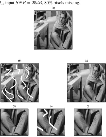
Fig. 2. Examples with Lena and Barbara. Dictionary: curvelets+LDCT, penalty: l1, input SN R = 30dB, 20%
pixels missing.
To further illustrate the power of the ECM inpainting algorithm, we applied it to the Barbara textured image. As stationary textures are efficiently represented by the local DCT, the dictionary contained both the curvelet (for the geometry part) and the LDCT transforms. Again, the l1
penalty was used. The result is portrayed in Fig.2. The algorithm is not only able to recover the geometric part (cartoon), but particularly performs well inside the difficult
textured areas, e.g. trousers.
The algorithm was finally applied to a real photograph of a parrot, where we wanted to remove the grid of the cage to virtually free the bird. The mask of the grid was manu-ally plotted. The result is shown in Fig.3. Here, the dictio-nary contained the undecimated DWT and LDCT, penalty: l1. For comparative purposes, inpainting results of a
PDE-based method [8] are reported. The main differences be-tween the two approaches are essentially concentrated the ”textured” area in the vicinity of the parrot’s eye.
Fig. 3. Original (left), ECM inpainting (middle) and PDE inpainting (right).
4. CONCLUSION
A novel, fast and flexible inpainting algorithm has been presented. Its theoretical properties were also derived. Sev-eral interesting perspectives of this work are under inves-tigation. We can cite the extension to any dictionary and formal investigation of the influence of the regularization parameter on the convergence the algorithm (path follow-ing/homotopy continuation). Extension to multi-valued images (e.g. hyper-spectral data) is also an important as-pect that is the focus of our current research.
5. REFERENCES
[1] M. Bertalm`ıo, G. Sapiro, V. Caselles, and C. Ballester., “Image inpainting,” in
SIGGRAPH 2000, New Orleans, USA, 2000, vol. 34, pp. 417–424.
[2] T. Chan and J. Shen, “Mathematical models for local non-texture inpainting,”
SIAM J. Appl. Math, vol. 62, no. 3, pp. 1019–1043, 2001.
[3] M. Elad, J.-L. Starck, P. Querre, and D. Donoho, “Simultaneous cartoon and texture image inpainting,” submitted to ACHA, 2004.
[4] J.-L. Starck, M. Elad, and D. Donoho, “Image decomposition via the combi-nation of sparse representatntions and variational approach,” IEEE Trans. Im.
Proc., p. in press, 2004.
[5] J.-L. Starck, M. Elad, and D.L. Donoho, “Redundant multiscale transforms and their application for morphological component analysis,” Advances in Imaging
and Electron Physics, vol. 132, 2004.
[6] X. L. Meng and D. B. Rubin, “Maximum likelihood estimation via the ecm algorithm: A general framework,” Biometrika, vol. 80, no. 2, pp. 267–278, 1993.
[7] C. Wu, “On the convergence properties of the em algorithm,” Ann. of Stat., vol. 11, pp. 95–103, 1983.
[8] D. Tschumperl´e and R. Deriche, “Vector-valued image regularization with pde’s : A common framework for different applications,” IEEE Trans. PAMI, vol. 27, no. 27, pp. 506–517, 2005.