The location and rate of dayside reconnection during an interval of southward interplanetary magnetic field

HAL Id: hal-00329265

https://hal.archives-ouvertes.fr/hal-00329265

Submitted on 1 Jan 2003

HAL is a multi-disciplinary open access

archive for the deposit and dissemination of

sci-entific research documents, whether they are

pub-lished or not. The documents may come from

teaching and research institutions in France or

abroad, or from public or private research centers.

L’archive ouverte pluridisciplinaire HAL, est

destinée au dépôt et à la diffusion de documents

scientifiques de niveau recherche, publiés ou non,

émanant des établissements d’enseignement et de

recherche français ou étrangers, des laboratoires

publics ou privés.

interval of southward interplanetary magnetic field

M. Pinnock, G. Chisham, I. J. Coleman, M. P. Freeman, M. Hairston, J.-P.

Villain

To cite this version:

M. Pinnock, G. Chisham, I. J. Coleman, M. P. Freeman, M. Hairston, et al.. The location and

rate of dayside reconnection during an interval of southward interplanetary magnetic field. Annales

Geophysicae, European Geosciences Union, 2003, 21 (7), pp.1467-1482. �hal-00329265�

Annales

Geophysicae

The location and rate of dayside reconnection during an interval of

southward interplanetary magnetic field

M. Pinnock1, G. Chisham1, I. J. Coleman1, M. P. Freeman1, M. Hairston2, and J.-P. Villain3

1_{British Antarctic Survey, Natural Environment Research Council, High Cross, Madingley Road, Cambridge, CB3 0ET, UK} 2_{Center for Space Sciences, Univ. of Texas at Dallas, Richardson, Texas, USA}

3_{LPCE/CNRS, 3A Av. De la Recherche Scientifique, 45071 Orleans Cedex, France}

Received: 27 August 2002 – Revised: 9 January 2003 – Accepted: 11 February 2003

Abstract. Using ionospheric data from the SuperDARN radar network and a DMSP satellite we obtain a comprehen-sive description of the spatial and temporal pattern of day-side reconnection. During a period of southward interplane-tary magnetic field (IMF), the data are used to determine the location of the ionospheric projection of the dayside magne-topause reconnection X-line. From the flow of plasma across the projected X-line, we derive the reconnection rate across 7 h of longitude and estimate it for the total length of the X-line footprint, which was found to be 10 h of longitude. Us-ing the Tsyganenko 96 magnetic field model, the ionospheric data are mapped to the magnetopause, in order to provide an estimate of the extent of the reconnection X-line. This is found to be ∼38 RE in extent, spanning the whole dayside

magnetopause from dawn to dusk flank. Our results are com-pared with previously reported encounters by the Equator-S and Geotail spacecraft with a reconnecting magnetopause, near the dawn flank, for the same period. The SuperDARN observations allow the satellite data to be set in the context of the whole magnetopause reconnection X-line. The total po-tential associated with dayside reconnection was ∼150 kV. The reconnection signatures detected by the Equator-S satel-lite mapped to a region in the ionosphere showing continu-ous flow across the polar cap boundary, but the reconnection rate was variable and showed a clear spatial variation, with a distinct minimum at 14:00 magnetic local time which was present throughout the 30-min study period.

Key words. Magnetospheric physics (magnetopause, cusp

and boundary layers; magnetosphere-ionoshere interactions) – Space plasma physics (magnetic reconnection)

1 Introduction

Understanding the transfer of solar wind momentum and plasma across the boundary of the dayside magnetopause is of prime importance in quantifying the impact of the solar

Correspondence to: M. Pinnock (M.Pinnock@bas.ac.uk)

wind on the Earth’s magnetosphere. While a good qualitative understanding of the processes involved has been achieved, considerable progress is still required before it can be reli-ably modeled and used for predictive purposes in applica-tions such as space weather forecasting. Most of the studies of the rate of momentum transfer have been performed at a single point on the magnetopause (e.g. Sonnerup et al., 1981) or in the ionosphere (e.g. de la Beaujardi`ere et al., 1991). Limited spatial coverage of the X-line has been achieved in some studies, for example, over a 2-h segment of the iono-sphere (Baker et al., 1997). In this paper we report observa-tions that encompass ∼70% of the dayside merging region, with a time resolution of 2 minutes, using ionospheric tech-niques.

The rate of magnetic reconnection in geospace is best monitored in the ionosphere. A snapshot measurement in-situ, at the reconnection X-line, can be made, but prolonged measurement is practically impossible due to our lack of knowledge of where the X-lines are, the variability in their position and the inability to keep a spacecraft there. At present, it is only in the ionosphere, where the cusp magnetic field topology causes dayside magnetopause phenomena to be focused in 3–6 hours of magnetic local time (Crooker and Toffoletto, 1995), that the area containing the footprint of the X-line (the merging line) can be monitored continuously. Traditionally, the reconnection rate has been measured in the ionosphere by the potential difference across the open field line region in the dawn-dusk meridian using polar orbiting spacecraft (Reiff et al., 1981). These measurements are lim-ited by their 1-D orbital trajectory (that does not always in-tercept the ends of the projected X-line) and their low reso-lution in time due to the ∼100-min spacecraft orbit. Such a sampling rate means that they cannot capture transient and localised reconnection phenomena that have been reported from ground-based experiments (e.g. Neudegg et al., 1999).

More recently, improved resolution has come from using a network of magnetometers, radars and spacecraft to con-struct the electric potential distribution across much of the high-latitude ionosphere and has provided useful information

Fig. 1. Geographic map showing the fields-of-view of the five

Su-perDARN radars used in the study. Geomagnetic latitudes from 50 to 80◦latitude are shown with bold lines, the faint lines show ge-ographic latitude over the same latitude range. The transit of the DMSP F13 satellite between 13:24 and 13:38 UT is shown by the dashed line. The bold magnetic meridian line (bottom left quadrant of the figure) marks magnetic noon at 13:30 UT.

on the large-scale ionospheric convection (e.g. Ridley et al., 1997). Even so, some uncertainties arise from the magne-tometer inversion method and spatial interpolation. Further-more, measurement of the ionospheric electric field alone is not sufficient to measure the dayside and nightside recon-nection rates. To measure the reconrecon-nection rate it is nec-essary to identify the ionospheric projection of the dayside and nightside X-lines and measure the potential differences along them in their rest frame (e.g. Freeman and Southwood, 1988; de la Beaujardi`ere et al., 1991). It is expected that the footprints of the X-lines vary in location on a time scale of minutes and by many 10s of kilometres (Cowley and Lock-wood, 1992), hence the need to reference the plasma flows to the rest frame of the X-lines. To achieve this measure-ment is difficult, as it usually requires a conjunction of at least two observing instruments; one to determine the foot-print of the X-line and a second to measure the plasma flow. Blanchard et al. (2001) have shown how a single incoherent scatter radar can be used to measure the reconnection rate at a single meridian. Studies by Baker et al. (1997) and Pinnock et al. (1999) demonstrated the ability of the radars of the Su-per Dual Auroral Radar Network (SuSu-perDARN) to Su-perform the measurement, the greater field of view of a single Super-DARN radar extending the coverage to ∼2 h of MLT. Global auroral images can also be used as a proxy for the polar cap boundary and the expansion and contraction of the polar cap area monitored through the substorm cycle (e.g. Brittnacher

et al., 1999). If combined with plasma flow measurements, then the reconnection rate could be estimated.

Phan et al. (2000) reported observations by the Geotail and Equator-S satellites of bi-directional plasma jets in the dawn-side low-latitude magnetopause, during a period of south-ward IMF. The repeated encounters with the jets over more than one hour indicated that reconnection was active much of the time, with its site remaining quasi-stationary near the equator. They argued for the existence of a stable and ex-tended reconnection X-line spanning the entire dayside mag-netopause. Partial confirmation of this hypothesis was pro-vided by Phan et al. (2001), which used SuperDARN radar data from the noon sector to confirm that subsolar reconnec-tion was occurring in the same period.

In this paper we use a network of the Northern Hemisphere SuperDARN radars and an overpass of the Defense Meteo-rological Satellite Program (DMSP) F13 satellite (see Fig. 1) to investigate the dayside reconnection rate across a wide longitudinal range (∼7 h of MLT). Using a magnetic field model, the ionospheric footprint of the reconnection X-line is mapped to the magnetopause surface. From this we de-termine where, and at what rate, reconnection occurs on the magnetopause with an unprecedented spatial coverage and resolution. This allows us to place the Phan et al. (2000, 2001) observations in the context of the whole dayside mag-netopause reconnection rate. We find evidence for one of the longest reconnection X-lines ever reported.

2 Observations

2.1 Event overview

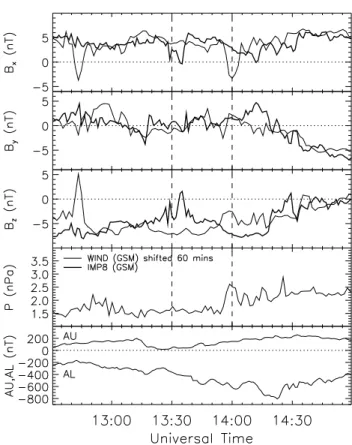
Figure 2 shows the IMF observed by the Wind (light line) and IMP–8 (dark line) spacecraft, the solar wind dynamic pres-sure meapres-sured by Wind, and the AU and AL auroral elec-trojet indices, for the period 12:30 to 15:00 UT on 11 Febru-ary 1998. The Wind spacecraft position at 13:30 UT was X = 235.4 RE, Y = 2.2 RE, Z = −31.4 RE in geocentric

solar magnetospheric (GSM) coordinates. Its data have been lagged by 60 min to give the best correlation with the data from IMP-8, whose position at 13:30 UT was X = 11.8 RE,

Y = −29.4 RE, Z = 0.3 RE in GSM coordinates. The

IMF Bz component became negative at ∼12:00 UT (at the

IMP–8 spacecraft) and remained negative until ∼15:00 UT, although there are some brief (few minutes), localized (i.e. only seen at IMP-8 or Wind) excursions to Bz positive (e.g.

at 13:35 UT). IMF Byis close to zero until 14:25 UT, when it

trends to ∼−6 nT at 15:00 UT. IMF Bxis ∼4 nT throughout,

with some short-lived, localized, excursions to zero or neg-ative values. Although there is evidence for some structure in the solar wind, this is relatively short lived. The period between 13:30 and 14:00 UT (vertical lines in Fig. 2) studied in this paper is thus best characterized by purely southward IMF.

The solar wind dynamic pressure was fairly typical at ∼1.6 nPa until 13:55 UT and then increased to ∼2 nPa. In

the period from 13:30 to 13:55 UT the variability in the pres-sure was typically not greater than 20%.

The AL electrojet index shows steadily increasing ac-tivity through the period. Particle flux data from the Los Alamos National Laboratory (LANL) 1994–84 spacecraft (not shown), in the 20:00 MLT sector at 13:30 UT, show no clear substorm particle injection signature until ∼16:25 UT. A weak, low electron energy particle injection signature was observed by the LANL 1997A satellite at ∼15:00 UT in the 19:00 MLT sector. However, the magnetogram from Col-lege, Alaska (not shown), at 22:40 MLT at 13:30 UT, shows a 500 nT negative bay in the H component commencing at 13:24 UT and peaking at 14:05 UT. The onset of the bay is very rapid and typical of that associated with a substorm on-set.

The Northern Hemisphere SuperDARN radars had their best scatter conditions in the interval 13:30 to 14:00 UT, so this forms the core time of this study.

2.2 Deriving convection maps from SuperDARN radars

SuperDARN is a network of coherent scatter high fre-quency (HF) radars (Greenwald et al., 1995) which measure backscatter from field-aligned, decameter-scale ionospheric irregularities. SuperDARN’s primary aim is to study the global ionospheric convection pattern at high latitudes. Sub-ject to achieving the backscatter condition, each radar can image 2–3 h of magnetic local time in the region of the po-lar cap boundary. The radars measure, in the F-region, the line-of-sight plasma velocity drift (Villain et al., 1985; Ruo-honiemi et al., 1987) and its spectral characteristics. The fields-of-view of the radars used in this study are shown in Fig. 1; this study predates the deployment of all 9 radars now operating in the Northern Hemisphere.

Many of the SuperDARN radars have overlapping fields-of-view which allow the estimation of unambiguous field-perpendicular velocity vectors, by combining coincident line-of-sight velocity measurements. However, overlapping scatter is not always present, so to maximize the use of all available line-of-sight data, the technique of global convec-tion mapping (Ruohoniemi and Baker, 1998) was developed. SuperDARN global convection maps are produced by fit-ting line-of-sight velocity data from the radars to an expan-sion of an electrostatic potential function, expressed in terms of spherical harmonics. Prior to this fitting process, radar data which are identified as groundscatter or which do not ex-ceed a certain minimum velocity (typically 35 m/s) or signal-to-noise ratio (typically 3 dB) are removed. This filtering process can sometimes fail to reject line-of-sight velocity data which do not relate to the convection electric field, e.g. ground scatter mixed with ionospheric scatter or E-region scatter which is limited to the ion acoustic velocity. Addi-tional techniques have been developed to ensure that these are removed (Chisham and Pinnock, 2002) and are employed here. The remaining line-of-sight velocity data are spatially and temporally median filtered. These data are then mapped

Fig. 2. Overview of the geophysical conditions on 11 February

1998. The dashed vertical lines in each panel mark the period of the reconnection analysis. The top three panels show the interplan-etary magnetic field measured by the Wind (faint line) and IMP-8 (bold line) spacecraft. The Wind data have been lagged 60 min in time to allow for the propagation time from Wind to IMP-8 (see text for position of the spacecraft). The fourth panel shows the solar wind dynamic pressure determined from Wind data, lagged by 60 min. The fifth panel shows the AU and AL indices for the period.

on to a geomagnetic coordinate grid encompassing the polar region (see Ruohoniemi and Baker, 1998 for full details).

In this study, the radar data have been supplemented with the along- and across-track plasma drift velocities from the DMSP F13 satellite (Retarding Potential Analyzer (RPA) and Ion Drift Meter instruments, respectively). The satellite tra-versed the northern polar cap between 13:24 and 13:37 UT (see Fig. 1) and went from ∼17:00 MLT to 06:00 MLT, reaching a peak geomagnetic latitude of 85◦N. The Alti-tude Adjusted Corrected Geomagnetic (AACGM) coordinate system, a development of the Polar Anglo-American Con-jugate Experiment geomagnetic coordinate system of Baker and Wing (1989), is used throughout this study. The satellite plasma drift data taken during each two-minute radar scan period have been processed using the same median filter-ing and griddfilter-ing technique as described in Ruohoniemi and Baker (1998), combined with the radar data, and the potential mapping solution obtained. The DMSP data provide valu-able additional information, particularly in the 06:00 MLT sector, where almost no radar scatter exists. The DMSP drift data have been examined carefully to remove corrupt

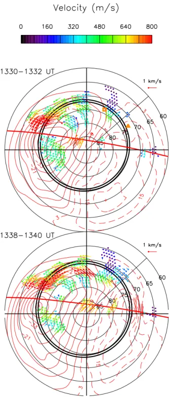
Fig. 3. Samples of the SuperDARN equipotential contour maps

for two periods, with radar determined “true vectors” and satellite plasma drift vectors overlaid, both colour-coded according to mag-nitude. The path of the DMSP F13 satellite in the interval from 13:24 to 13:38 UT is shown by the red line. The orange square and triangle in Fig. 3a mark the location to which the Equator-S and Geotail satellites map at 13:30 UT, respectively. The longitude line in the upper right quadrant of each picture marks the 0◦E location.

data. In particular, data from below 62 degrees latitude in the 06:00 MLT sector were invalid because the plasma

den-sity was too low to give reliable values. Also, examination of the RPA current and voltage curves showed that in the interval between 69◦_{and 65}◦_{N geomagnetic latitude in the}

06:00 MLT sector some data points were not of good enough quality to give reliable values. These too have been removed from our analysis. Finally, the drift data (measured in the in-ertial reference frame) are translated to the corotating frame (the same reference frame as the radar data) before being combined with the radar data.

To constrain the solution effectively in regions where little or no radar or satellite data are available, a statistical model (Ruohoniemi and Greenwald, 1996) is used to augment the data. The choice of statistical model is based on the prevail-ing IMF conditions and, although havprevail-ing some influence on the global solution, generally has little influence on the solu-tion in regions where data exist (Shepherd and Ruohoniemi, 2000). The fitting is then performed on the combined data set and the best fit determined by a least-squares method. The fitting is dependent on the following user-selected pa-rameters: (1) the order of the spherical harmonic fit, and (2) the spatial extent over which the fit is performed. Higher or-der fits reproduce better mesoscale features of the convection and reduce the uncertainty of the fit, but are more compu-tationally intensive. In this study 11th order fits have been used. Changing the spatial extent of the fitting can change the global nature of the solution but rarely has a significant effect on mesoscale variations. The solution provides an es-timate of the convection electric field across the polar region of the ionosphere and can be used to study its large-scale characteristics (e.g. the cross-polar cap potential, Shepherd and Ruohoniemi, 2000) or its mesoscale features (e.g. flow vortices, convection reversal boundaries).

The solution is good in regions where radar backscatter exists but one must be careful in reaching conclusions from areas were the flows are mainly determined by the statistical convection model. For this reason, we only derive the recon-nection rate at longitudes where radar data are present. The plasma flow vectors used in this study are termed “true vec-tors”; they are derived from the radar line-of-sight velocity measurement, combined with the velocity component trans-verse to the radar beam, which is derived from the equipo-tential contour pattern given by the convection fitting process (see Chisham et al., 2002, Appendix A). Provan et al. (2002) showed that the “true vectors” are a better estimate of the magnitude of the flow than are “fitted” vectors (which are determined solely from the potential contour map).

Figure 3 shows two sample convection patterns, for the intervals, 13:30–13:32 UT (Fig. 3a) and 13:38–13:40 UT (Fig. 3b). In these plots the radar scatter exists wherever a radar “true vector” is plotted. Note that vectors shown as lo-cated on the path of the DMSP F13 satellite (red line) are from its ion drift data. In the 13:30–13:32 UT pattern these are located between 82 and 86◦N latitude in the 15:00 MLT sector; in the 13:38–13:40 UT pattern they are located be-tween 69 and 72◦N latitude in the 06:00 MLT sector. Outside these regions only the equipotential contours derived from the data fitting process are shown. The quality of the global

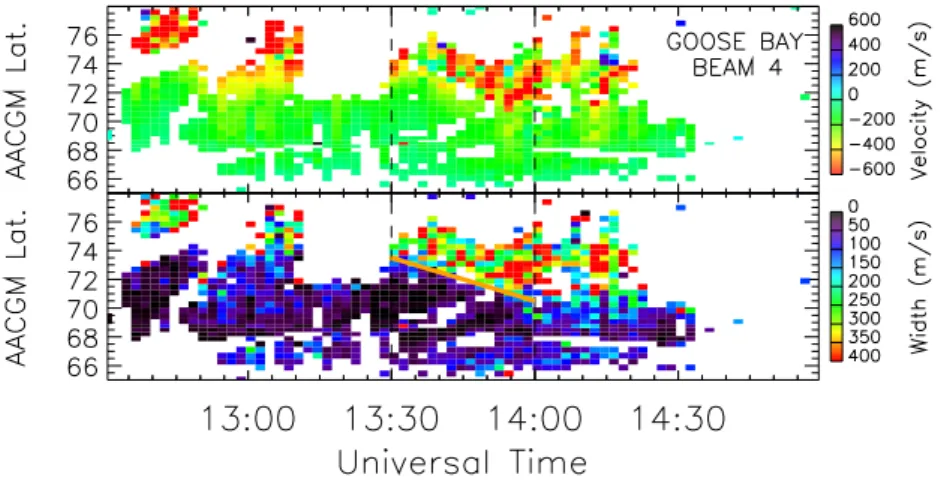
Fig. 4. The two panels show the

line-of-sight Doppler velocity (upper panel) and the Doppler spectral width (lower panel) measured by the Goose Bay radar on beam 4 (aligned with the mag-netic meridian). The orange sloping line on the lower panel marks the equa-torward movement of the boundary be-tween high and low spectral widths.

convection pattern fit to the radar and satellite data is mea-sured by a chi-squared parameter. The values for this are 0.9 and 1.3 for the 13:30–13:32 UT and 13:38–13:40 UT peri-ods, respectively, values that are usually taken as represent-ing a good fit (Ruohoniemi and Baker, 1998, p 20 803). 2.3 Locating the Polar Cap Boundary (PCB)

Accurately locating the ionospheric footprint of the magne-topause (the polar cap boundary) presents the greatest diffi-culty in any attempt to measure the reconnection rate. Lock-wood (1997) and Rodger (2000) have drawn attention to the uncertainties involved in using ionospheric proxies for the PCB on the dayside, such as convection reversal, particle pre-cipitation and auroral emission boundaries.

In this study, the location of the polar cap boundary for the period around 13:30 UT is found using satellite data near the dawn and dusk meridians and radar data from the pre-noon sector. In order to extrapolate the PCB to all dayside longi-tudes, a circle is fitted to these 3 points, which is the simplest continuous, closed shape that can connect them. Then, the radius of this circular PCB is incremented linearly with time between 13:30 and 14:00 UT, to agree with the linear latitudi-nal motion of the PCB in the pre-noon sector detected by the radar (see below). This provides a PCB location to be used with the plasma flow vectors derived every two minutes.

The assumption that the arc of a circle can approximate the PCB across the local time sector spanned by the radar and satellite data (06:00–17:00 MLT) and over the 30-min interval of interest is justified by reference to previous obser-vations of the poleward boundary of the auroral oval that is a proxy for the PCB. Holzworth and Meng (1975), in deriving a mathematical expression for the Feldstein (1963) statistical oval, found that the poleward boundary of the auroral oval is approximated to zero order by a circle offset from the mag-netic pole, for all geomagmag-netic activity levels. They verified this conclusion using quiet time (i.e. absence of substorms) DMSP satellite auroral images. Higher order components were found, but the magnitude of these perturbations on the dayside gives a maximum tilt of the PCB of the order of 10 degrees with respect to the zero order circle (see Pinnock

et al., 1999, p. 447 for discussion of this), which results in an error of <20% in determining the reconnection electric field for a flow vector of any magnitude within ± 45◦of the normal to the assumed circular PCB. Significant perturba-tions of the auroral oval shape are found for IMF Bz

north-ward (Hones et al., 1989), significant IMF By component,

and after substorm onset (Frank and Craven, 1988). Such conditions are absent during the study presented here, which takes place after 90 min of steady Bzsouthward with nearly

zero IMF By component, in an interval of steadily

increas-ing AL index consistent with a growincreas-ing DP2 current system, and with no substorm particle injections observed by geosyn-chronous satellites. These substorm growth phase conditions are optimal for observing a poleward boundary of the day-side auroral oval that approximates a circle (e.g. examples shown in Brittnacher et al., 1999).

In regions (e.g. dusk sector) where the flow vector is not within 45◦of normal to the assumed circular PCB it should be borne in mind that the radar’s “true vectors” include a line-of-sight velocity measurement (from a single radar beam) that is very close to orthogonal to the PCB and thus provides a direct measurement (rather than a derived one) of the com-ponent critical for the reconnection electric field value. This point is returned to in Sect. 2.5.1; the use of more zonal point-ing radar beams is shown to significantly underestimate the reconnection electric field.

The location of the boundary and the inflation rate of the polar cap have been fixed in the ∼10:30 MLT sector, us-ing the Doppler spectral width characteristics of the Goose Bay radar backscatter. The equatorward edge of radar scat-ter showing large Doppler spectral widths, scat-termed the spec-tral width boundary (SWB), has been shown to be coinci-dent with the equatorward edge of the cusp particle precipi-tation (Baker et al., 1990, 1995) for a southward interplane-tary magnetic field (IMF). Andr´e et al. (1999) have identified the cause of this large Doppler spectral width as due to the intense Pc1 wave activity present in the cusp.

The Goose Bay radar data from beam 4, aligned along the magnetic meridian, is shown in Fig. 4. This shows a mixture of ground scatter (low velocity (green) and low

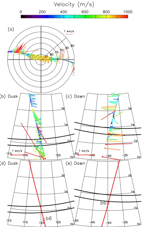
Fig. 5. Observations of the plasma drift by DMSP F13 satellite (at 845 km altitude) around 13:30 UT. The cross-track and ram direction data

have been combined to produce a vector. Panel (a) shows all the data from the transit of the northern polar cap. Panels (b) and (c) show sections of the afternoon and morning plasma flows respectively. The bold lines show the polar cap boundary used in our measurements. The b6 particle precipitation boundary (see text) is marked in panels (d) and (e) with a red square.

spectral width (blue/black)) and ionospheric scatter seen at higher latitudes (≥ 70◦_{N). The high-latitude scatter shows}

characteristics consistent with a Bz southward period: large

poleward velocities (red/yellow) with large Doppler spectral widths (red/green) characteristic of the cusp scatter. This

scatter migrates steadily equatorward through the study pe-riod. This allows us to determine the location of the PCB in this time sector and also its temporal variation. At 13:00 UT (09:43 MLT), the SWB is at ∼74◦_{N. The FAST and DMSP}

Goose Bay radar field-of-view at 13:02 and 12:54 UT, re-spectively. From the particle precipitation characteristics (not shown) observed by both spacecraft, the equatorward boundary of the cusp particle precipitation is located at 74◦N latitude, providing independent verification of the PCB de-rived from the Goose Bay data (although at a later local time). At 13:30 UT, the SWB was located at ∼73◦N and then mi-grated steadily equatorward to 70◦N latitude at 14:00 UT, an equatorward motion of 185 ms−1. This equatorward migra-tion is consistent with the prevailing IMF Bzsouthward

con-ditions. Phan et al. (2001), using SWB data from the Halley, Antarctica, SuperDARN radar (conjugate to the Goose Bay radar), had estimated the polar cap equatorward expansion to be at the rate of 150 ms−1. The Halley radar data had no low spectral width data (i.e. all the scatter showed spectral widths consistent with cusp scatter) so the determination of the SWB from its data must be considered to be less accurate. The southern SWB was typically one degree poleward of the northern SWB, consistent with the prevailing dipole tilt con-ditions at the time which would cause the summer (southern) cusp to be at higher latitudes (Newell and Meng, 1989).

Rodger and Pinnock (1997) noted that the equatorward edge of the cusp particle precipitation is offset from the PCB due to the time of flight of the cusp ions and the poleward convection of the flux tubes containing the precipitating par-ticles. Any phenomena (e.g. cusp 630 nm auroral emis-sions or radar Doppler spectral width boundary) related to the cusp precipitation will also be offset from the true loca-tion of the PCB. Pinnock and Rodger (2001) illustrated the self-consistency of this approach, deriving typical cusp ion travel times from SWB and convection data available from the SuperDARN radars.

An average offset between the location of the SWB and the true location of the PCB has been derived by the follow-ing method. The field-aligned distance traveled by the pre-cipitating ions, from the equatorial magnetopause reconnec-tion X-line to the ionosphere, was calculated from the Tsyga-nenko 1996 magnetospheric field model (TsygaTsyga-nenko, 1995, 1996; Tsyganenko and Stern, 1996, hereafter referred to as T96) and is 14.9 RE. The particle travel time is assumed to

be characteristic of that for 3 keV protons at 0◦pitch angle, typical of those found at the equatorward edge of the cusp (Newell and Meng, 1991). These will have a time of flight from the magnetopause reconnection site to the ionosphere of 125 s. The mean of the poleward convection measured directly by the Goose Bay radar line-of-sight velocities on beam 4, at the latitude of the SWB between 13:30 UT and 14:00 UT, was calculated to be 330 m/s, (standard deviation of 89 m/s). To this we add the velocity of the SWB, 185 m/s (the boundary is moving equatorward at the same time as the flux tube is convecting polewards) to arrive at an effective poleward velocity component of 515 m/s. From these val-ues we find that the polar cap boundary needs to be offset by 0.58◦equatorward from the SWB location. Thus, at 13:30 UT, the PCB is located at 72.4◦N at 10:14 MLT; at 14:00 UT it is at 69.4◦N latitude at 10:44 MLT.

This estimate of the dayside polar cap boundary location

at ∼10:30 MLT is supplemented by the PCB determined by examining data taken in the dawn and dusk sectors by the DMSP F13 pass between 13:24 and 13:37 UT. Figure 5 shows a summary of the plasma drift data, panel (5a), and expanded views of the drift data in the dusk and dawn sec-tors, panels (5b) and (5c). The particle boundary “b6”, de-rived using the classification scheme of Newell et al. (1996) is shown by the red squares in panels (5d) and (5e). This boundary is the poleward limit of sub-visual auroral driz-zle, which, in both the dawn and dusk sectors of this pass, is within 0.1 to 0.2◦of latitude of the onset of polar rain precip-itation. We have also examined the individual ion and elec-tron spectrograms to verify this identification. In the dawn sector the particle boundary b6 agrees to within 0.4◦of lat-itude with the location of the convection reversal boundary (CRB), determined as the latitude at which persistent sun-ward flow was established. Taking the CRB as defining the PCB, this locates it at 73.6◦_{N/06:16 MLT at 13:38 UT. In the}

dusk sector there is a greater discrepancy between the CRB (72.2◦N/ 16:29 MLT at 13:26 UT) and the particle boundary b6 (71.0◦N). We note that the region poleward of b6 and up to 72.2◦ latitude is all on sunward convecting plasma. We have decided to use the CRB as the best estimate of the PCB in the dusk sector. The CRB latitudes have been linearly in-terpolated in time to give their latitude at 13:30 UT, assuming the polar cap boundary expansion was at the rate of 185 m/s equatorward derived from the radar data. After fitting a cir-cle to the three PCB locations described above, Fig. 6 shows the boundary location as a function of MLT (solid line) at 13:30 UT and 14:00 UT.

We can use the encounters with the magnetopause by the Equator-S and Geotail satellites in this period, as reported by Phan et al. (2000), as a means of checking the ionospheric estimate of the boundary location. The satellite data allow us to set some limitations on the location of the magnetopause. The T96 model is then used to locate the magnetopause foot-print in the ionosphere. This is a coarse check: there is a large degree of uncertainty in locating the moving magnetopause with respect to the spacecraft and also the uncertainty asso-ciated with the field line mapping.

Phan et al. (2000, their Fig. 2 and text) suggest that at 13:30 UT the two spacecraft make occasional encounters with the magnetopause, but that the Geotail spacecraft is in-side the magnetosphere while Equator-S is predominantly in the magnetosheath. Thus, the magnetopause passed between the two spacecraft (which are separated by ∼3 RE in the X

GSM plane, on the dawn side of the magnetopause). Using this fact, the solar wind dynamic pressure (Psw) input to the

T96 model has been adjusted until the location of the mag-netopause passed between the two spacecraft. It was found that at 13:30 UT, the Psw had to be set to 4 nPa (in contrast

to the Pswmeasured by Wind of 1.7 nPa) to achieve this. (A

suitable fit to the satellite data could be obtained over a range of solar wind pressures between 3.2 nPa and 4.7 nPa.) The location of the magnetopause was then mapped into the iono-sphere by field-line tracing, to give an estimate of the location of the PCB. This exercise has been repeated for 14:00 UT.

6 8 10 12 14 16

MLT (h)

Latitude (

)

Fig. 6. The location of the polar cap boundary at 13:30 UT (upper

curve, solid line), estimated from the Goose Bay radar data (triangle symbol) and the convection reversal boundary derived from DMSP F13 plasma drift data (two circles). The latitude of the boundary (y-axis) is plotted as a function of magnetic local time (x-(y-axis). The lower curve (solid line) shows the location of the PCB at 14:00 UT, determined from the polar cap expansion rate given by the Goose Bay radar data. The triangle symbol represents the location of the polar cap boundary derived from the Goose Bay radar data at 14:00 UT. The two dash-dot lines represent the location of the PCB derived from the estimated magnetopause location (using Equator-S and Geotail satellite data) when mapped to the ionosphere using the Tsyganenko 1996 magnetospheric field model. The high-latitude line represents the boundary at 13:30 UT, the lower latitude line the boundary at 14:00 UT.

At that time both spacecraft are in the magnetosheath and Equator-S makes no magnetopause encounters whilst Geo-tail is still making frequent encounters, suggesting that it is just outside the magnetopause. In this case the Pswhad to be

set to 5 nPa to match the spacecraft data with the T96 model magnetopause.

Having to use larger Psw values than actually measured,

in order to fit the satellite data, is not surprising. The T96 model has an ellipsoid magnetopause whose parameters are controlled solely by the dynamic pressure. It is well estab-lished that the IMF Bz component also controls the location

of the magnetopause (Roelof and Sibeck, 1993). It has also become clear (Shue et al., 2001) that the IMF history in-fluences the location of the magnetopause. The IMF had been southward for 1.5 h prior to our observations and hence, magnetopause erosion will have been ongoing, displacing the magnetopause earthward from that predicted solely by the solar wind pressure term. Our findings are pertinent to papers attempting conjugate observations between magne-topause spacecraft and the ionosphere, for example, Neudegg et al. (1999). In particular, in the dawn sector the variation of the solar wind pressure between the measured value at

Wind (1.7 nPa) and the values we have used above make a considerable difference to the local time sector of the iono-spheric footprint of the Equator-S satellite (07:30 MLT cf. 09:15 MLT).

The results of this mapping are shown in Fig. 6 as dash-dot lines, with the high-latitude curve representing for 13:30 UT. This curve agrees with the PCB estimate derived from iono-spheric data to within 0.6◦_{and, given the limitations of}

lo-cating the moving magnetopause, provides confidence in our ionospheric data. The mapping also confirms the equator-ward expansion of the PCB, although the curve for 14:00 UT is 0.8◦ higher in latitude (at 10:44 MLT) than that derived from the Goose Bay radar data. The 14:00 UT mapping curve represents an upper limit for the PCB location, as by this time, both spacecraft are in the magnetosheath and there is, therefore, a higher degree of uncertainty in locating the magnetopause.

The location of the polar cap boundary for each 2 min radar scan period is determined by moving the polar cap boundary determined at 13:30 UT (solid, upper curve in Fig. 6) equatorward at a rate of 185 m/s for the time elapsed since 13:30 UT. The location of the SWB by the radar has an error of ± one range gate (45 km; see Andr´e et al., 1997; Pinnock et al., 1999, p. 445) and we have taken this as the uncertainty in our polar cap boundary location.

2.4 Measuring the reconnection electric field

As stated by de la Beaujardi`ere et al. (1991), the rate at which flux is added to the polar cap and its equivalence to the recon-nection electric field (Erec) for a particular segment (dl ) of

the PCB is represented by:

dF

dt =B × v

0_·

dl = Erec·dl, (1)

where dF_dt is the flux transfer rate, B is the local magnetic field and v0 is the horizontal velocity of the plasma in the rest frame of the separatrix. Equation (1) in our analysis thus becomes:

dF

dt =Erec·dl = Bz(ν ·cos θ − u) dl, (2) where ν is the plasma velocity in the Earth’s frame, Bz is

the vertical component of the AACGM model field (at 300 km), θ is the angle between the plasma flow direction and the normal to the PCB and u is the velocity of the PCB, also in the normal direction. The value of v0 is derived in the following fashion:

1. At any particular longitude the true vector within the PCB uncertainty limits is identified;

2. The orientation of the PCB (its angle relative to a line of geomagnetic latitude) at this longitude is determined from the PCB data points on either side of the longitude;

3. The flow orthogonal to the PCB is determined, ν · cos θ ; 4. The speed of the PCB (u), in the direction orthogonal to the orientation of the PCB, over the preceding two-minute interval is determined;

5. The flow across the PCB is combined with the velocity of the PCB to give v0 =ν·cos θ − u. Thus, equatorward motion of the separatrix will enhance the flow across it, poleward motion will reduce the flow across it.

The reconnection electric field,Erec, is then derived from

assuming:

Erec= −ν0×Bz. (3)

This Erecvalue applies over the longitude range, dl, defined

by the distance between the midpoints to the neighboring longitudes at the separatrix that have a true vector, in both directions. Where true vectors are continuous in coverage (e.g. Fig. 3a, ∼14:00 MLT to ∼16:00 MLT) this will be ap-proximately 50 km on either side of a vector (the radar beam width being approximately 100 km at this latitude). Note that where gaps exist in the radar backscatter coverage (e.g. Fig. 3a. ∼10:30 MLT to ∼12:00 MLT), the value of Ereccan

apply for a much greater distance (i.e. a larger dl).

By summing all the values along the dayside merging line, the total potential difference along the line, 8rec=P_iEreci·

dli, can be determined.

Note that Erec · dl has only been calculated between

the longitude limits set by where we have radar true vec-tors. These limits are between approximately 09:00 and 16:00 MLT. The equipotential contours in Fig. 3 suggest that flows across the boundary exist outside these limits. e.g. out to a limit of 17:00 MLT in the afternoon cell, as shown by the DMSP data (Fig. 5b), which shows poleward flow cross-ing the PCB. The morncross-ing cell flow limits are harder to de-termine because of the lack of data, but using the 13:38– 13:40 UT equipotential pattern (which has DMSP data defin-ing the morndefin-ing cell in the 06:00 MLT sector), it may ex-tend to 06:30 MLT. The DMSP data at 06:15 MLT shows no poleward flow crossing the boundary (Fig. 5c), but rather an equatorward flow, which would be consistent with a re-connection site at later local times, causing the boundary to move equatorward in this local time sector (Cowley and Lockwood, 1992).

2.5 The reconnection electric field

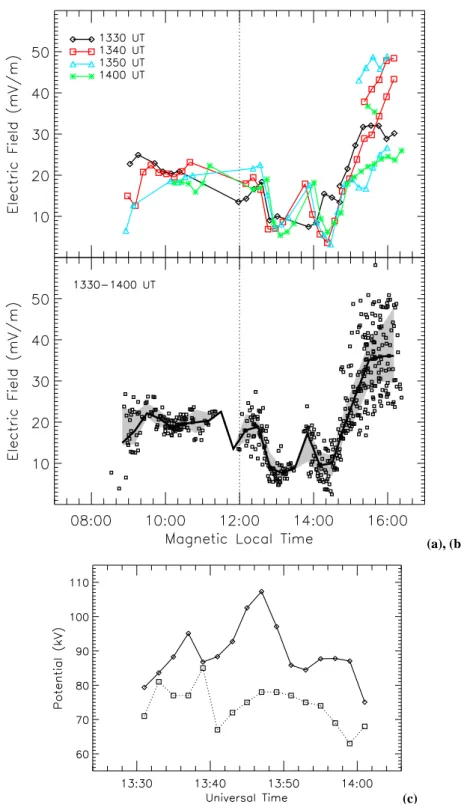
In Fig. 7 we present a summary of the reconnection electric field measurements derived from applying the above tech-nique to the SuperDARN radar data for the two-minute scans in the period 13:30 UT to 14:00 UT. The top panel shows the values as line plots for sample two-minute scans, plot-ted against the magnetic local time location of the measure-ments. Where more than one line from the same scan pe-riod exists (e.g. 13:40 UT scan in the 16:00 MLT sector), this is where data from more than one radar exists at a given location; it is thus possible to produce a vector from each

radar data set. The middle panel shows the Erec values

de-rived in the whole interval, with median and quartile values shown. The panels show that the distribution of the reconnec-tion electric field across the dayside merging line is remark-ably steady over the 30 min, except in the 15:00–16:00 MLT sector, where the spread between the upper and lower quar-tile reaches 18 mV/m. The mean reconnection electric field (all data points (Fig. 7b) in the interval 13:30–14:00 UT) is 22.0 mV/m.

The third panel (Fig. 7c), plotted against Universal Time, shows the variation of the dayside reconnection potential, 8rec, determined from the radar true vectors (solid line). The

extent to which the radar’s true vectors provide coverage across the whole dayside merging line will determine how close this value is to the total potential associated with day-side reconnection. The radar true vectors exist over a time sector spanning 7 h of MLT; the equipotential pattern shows this may be extended to 10.5 h of MLT, e.g. in Fig. 3b flow is crossing the boundary between 17:00 and 06:30 MLT. So it is possible that the radar’s true vectors can only provide the re-connection electric field over ∼67% of the merging line. The total potential measured by the radars varied between 75.07 and 107.3 kV, with a mean value of 89.3 kV. Also shown in Fig. 7c is the total cross polar cap potential (dashed line) de-termined from the fitted global equipotential pattern. This varied between 63 and 85 kV with a mean value of 69 kV. This can be compared with the value of 95 kV given by in-tegrating along the path of the DMSP F13 satellite for the interval 13:24 to 13:40 UT. The equipotential maps in Fig. 3 suggest that the satellite passed very close to the centers of the morning and afternoon convection cells and hence, pro-vided a good estimate of the total cross polar cap potential. The value of the total cross polar cap potential is examined further in the discussion section.

2.5.1 Errors and uncertainties

Flow vectors used to determine flow across the polar cap boundary are subject to the errors of the radar line-of-sight velocity (Vlos) measurements; data with errors greater than

200 m/s are excluded from the convection mapping process. The velocity component transverse to the radar beam, deter-mined from the global equipotential pattern, has an element of uncertainty associated with it that cannot be readily ex-pressed as an error measurement. This particular period has been subject to intense study, in terms of the quality of the fitted convection pattern, and is described in Chisham and Pinnock (2002). The reader is referred to that paper for de-tailed discussion.

We have used a smooth, circular polar cap boundary. An estimate of the likely maximum error arising from incorrectly determining the orientation of the PCB was given in Sect. 2.3 as being <20%. Small-scale motion of the boundary, both in the spatial and temporal sense, does exist (e.g. Sandholt et al., 1998). However, this motion occurs on a size comparable to the errors (±45 km) in locating the spectral width bound-ary in the radar data set. Pinnock et al. (1999) performed

(a), (b)

(c)

Fig. 7. Panel (a): The reconnection electric field (y-axis) measured at a range of MLTs (x-axis) for 4 radar scan periods. Panel (b): all the

reconnection electric field values measured from 13:30–14:00 UT. The solid line is the median reconnection electric field for a given MLT, the shading marks the upper and lower quartiles. Panel (c): the total reconnection potential (y-axis) measured across the dayside merging line sampled by the radar coverage (∼7 h of MLT, see text for discussion) over the UT period (x-axis) of the study is shown by the solid line. The total crosspolar cap potential, as determined by the convection mapping process, is shown by the dotted line.

a detailed study of the boundary motion, using the spectral width data from radars, and confirmed that boundary motions (within one scan period, 100 s) seldom exceeded the errors in the measurement. They used a highly smoothed

bound-ary in computing the reconnection electric field and noted that they still had measurements which accounted for close to 100% of the total cross polar cap potential measured by DMSP satellite, suggesting that no significant potential was

13.5 13.6 13.7 13.8 13.9 UT hour 10 14 18 22 Average Erec, mV/m

Fig. 8. The average reconnection electric field (Erec) in the

mag-netic longitude sector (0–15◦) conjugate to the Equator-S satellite as a function of universal time.

being omitted. We conclude that, while small-scale detail in the reconnection electric field may be missed, the value of the reconnection electric field over a period of several minutes is accurately quantified.

An estimate of the uncertainties involved can also be gained from polar cap boundary locations where data from more than one radar are available. This provides a “true vec-tor” from each radar and hence, more than one estimate of the reconnection electric field. This is shown in Fig. 7 by pairs of lines (same colour) in certain MLT sectors. From this it can be seen that while multiple radar measurements can agree to within ∼5 mV/m (e.g. 13:40 UT (red line) in Fig. 7a in the 15:00–16:00 MLT sector), disagreements can be in excess of 20 mV/m for measurements from one epoch (13:50 UT, blue line in Fig. 7a) in the 15:00–16:00 MLT sector. Careful inspection of these extreme examples shows that the radar (Iceland East) giving the low values has a zonal viewing di-rection, and the high values of Ereccome from a meridional

pointing radar (Finland). As the latter has beams that are or-thogonal to the PCB, their line-of-sight measurements (i.e. the raw data input to the convection modeling) are a direct measurement of the flow across the boundary. Inspection of these line-of-sight values in the vicinity of the boundary con-firms that the high Erec values are representative of the true

flow across the boundary. We have left the erroneous (lower Erec) values in the plots to illustrate the errors that may arise

when only zonal pointing radars are contributing data. 2.6 Mapping to the magnetopause

In order to relate the ionospheric measurements to recon-nection at the magnetopause, and the magnetopause obser-vations by the Geotail and Equator-S satellites (Phan et al., 2000), we have used the T96 model to perform field line

mapping in a manner identical to that described in Coleman et al. (2000).

The field line mapping has been done for 13:30 UT using the adjusted solar wind pressure value (4 nPa) as described in Sect. 2.3. The results of the mapping are shown in Fig. 3 (upper panel). The Geotail spacecraft (triangle symbol in Fig. 3) mapped to 08:00 MLT (and just equatorward of the PCB) while Equator-S was positioned at 10:30 MLT (and just poleward of the PCB).

The limits of the dayside merging line, taken as between 17:00 and 06:30 MLT and at the latitudes given by our polar cap boundary estimate, have been mapped out to the magne-topause and the points at which they cross the Z = 0 (equato-rial) plane have been determined. The duskward limit of the merging line maps to X = −0.3 RE, Y = 12.6 REGSM; the

dawnward limit to X = −9.0, Y = −15.5 RE GSM. This

means that the dayside reconnection X-line spans 38.2 RE

(in the Z = 0 plane) on the magnetopause surface of the T96 model. This result is very insensitive to the solar wind pres-sure value used; using the range of solar wind prespres-sures (3.2 to 4.7 nPa) given in Sect. 2.3 varies the X-line length by only 0.2 RE.

2.7 Satellite observations at the magnetopause

The Geotail satellite maps to a region where no ionospheric data is available (see Fig. 3, 07:40 MLT sector) but the Equator-S satellite maps into the Goose Bay and Stokkseyri (Iceland West) radars’ field-of-view, in the 09:00–10:00 MLT sector. Phan et al. (2000, their Fig. 2c), identified 3 plasma jets in the Equator-S data in the interval 13:30–14:00 UT, at 13:34, 13:40 and 13:45 UT.

From Fig. 7b it can be seen that the ionospheric recon-nection electric field is always above 0 mV/m in this sector. In Fig. 8 the average Erecvalue in the longitude sector

be-tween 0 and 15◦east magnetic longitude (08:45–09:45 MLT at 13:30 UT, the region closest to 10:30 MLT which has contiguous radar data) is plotted from 13:30–14:00 UT. Erec

varies considerably through the period, with peak values at 13:30, 13:36, 13:45 UT and 14:00 UT. If one notes that the PCB equatorward motion (185 m/s) is contributing nearly 10 mV/m to Erec, then from this base line level one can see

that the plasma is accelerated across the PCB in a series of surges.

3 Discussion

3.1 The longitudinal extent of the magnetopause reconnec-tion X-line

The SuperDARN radar data sets a lower limit of 7 h for the width of the dayside merging line. The equipotential patterns derived from the radar and DMSP F13 data show flow crossing the polar cap boundary from ∼06:30 MLT to ∼17:00 MLT, or 10.5 h of MLT.

It is possible to check for consistency within our data by noting that the polar cap boundary, in the noon sector, was

observed to move equatorward at the rate of 3◦ _{in 30 min}

(Fig. 4). Taking this expansion rate, and assuming a circu-lar pocircu-lar cap boundary, this equates to a flux transfer rate of 1.159 × 105T/s or, using Eq. (1), this equates to a mean potential of ∼116 kV. Taking this value, and the mean re-connection electric field measured by the radars (22.0 mV/m derived from the data shown in Fig. 7b), implies a dayside merging line of 5100 km. At a mean latitude of 72◦, this translates to a merging line that spans ∼10 h of MLT, in close agreement with the equipotential patterns.

We conclude that the dayside merging line on this day spanned ∼10 h of MLT, which magnetic field line mapping showed gave a magnetopause reconnection X-line of 38 RE

(Sect. 2.6). This gives an average reconnection electric field of ∼0.5 mV/m at the magnetopause. This is comparable to the average reconnection electric field produced from many satellite passes in the noon sector of the magnetopause (e.g. Lindqvist and Mozer, 1990).

A dayside merging line of 10 h MLT is very large com-pared to theoretical studies which have predicted a typical dayside merging line of ∼4 h of MLT for a cross-polar cap potential of 100 kV (e.g. Crooker and Toffoletto, 1995). Re-cent modeling work by Coleman et al. (2000) found that the dayside merging line predicted by the anti-parallel merging hypothesis varied with dipole tile angle; it ranged between 3 h (summer) and 8 h (winter) of MLT. Previous experimen-tal data have suggested values between 3 h (Pinnock and Rodger, 2001) and greater than 8 h of MLT (Crooker et al., 1991) for the dayside merging line in the ionosphere.

Observations of the length of the magnetopause X-line are extremely difficult to make. Lewis et al. (1998) and Yeo-man et al. (1999) used an indirect observational technique (expansion of the polar cap boundary combined with use of a reconnection model) to infer magnetopause X-lines of di-mension 12 and 27 RE, respectively. Original estimates of

the longitudinal extent of FTEs on the magnetopause were of the order of 1 RE (Russell and Elphic, 1979), but

subse-quently workers suggested a greater extent (e.g. Southwood et al., 1988). Lockwood and Davis (1996) argued for a mag-netopause X-line length of at least 3 h of MLT based on inter-pretation of longitudinal passes of DMSP satellites through the cusp ionosphere.

Statistical or synthesized convection patterns for south-ward IMF (e.g. Heppner and Maynard, 1987; Weimer, 1995; Ruohoniemi and Greenwald, 1996) do show flow rotating poleward and flowing anti-sunward over 81₂ to 11 h of MLT on the dayside, in closer agreement with our findings. We also note that Shepherd et al. (2000) suggested that if the reconnection X-line were to span the whole dayside magne-topause, as reported here, it could explain observations of the simultaneous response in ionospheric flows over a large range of MLTs following a southward turning of the IMF (e.g. Ridley et al., 1998). Our findings also support Lock-wood (1997) and Provan and Yeoman (1999), who consid-ered cusp particle precipitation observations and plasma flow data and concluded that the ionospheric projection of the

magnetopause X-line was wider than that predicted solely by cusp particle precipitation data (Newell and Meng, 1992). From the the discussion above, it is clear that the observa-tion reported here is at the extreme of previous measurements and assumptions. For a purely southward IMF both the com-ponent merging and the anti-parallel merging models pre-dict a reconnection X-line of maximum extent. Nishida and Maesawa (1971) have pointed out that for component merg-ing the length of the magnetopause X-line scales as roughly sin(2/2), where 2 is the angle between the magnetosheath and magnetospheric field lines (2 = 180◦ being the anti-parallel condition).

3.2 Longitudinal variation in reconnection rate

The distribution of the reconnection electric field, along the dayside merging line, retains stable characteristics through-out a 30-min study period. In a coarse sense, there is a gradi-ent along the merging line, with larger Erecvalues observed

at the eastern (afternoon) end. We do not have an explanation for this gradient. The reduction in Erecin the 14:00 MLT

sec-tor, to values below 10 mV/m, is an interesting feature. Note also that the variance in our measured reconnection rate is not great in this local time sector. The convection pattern (see Fig. 3) in the 14:00 MLT sector has equipotentials that are almost parallel to the modeled polar cap boundary, giv-ing sunward (return) flow and thus accountgiv-ing for the low Erec values. One possible explanation is that the

assump-tion of a circular polar cap boundary is in error in this sector and, therefore, the flow is not parallel to it. Just immedi-ately poleward of the modeled PCB, the equipotentials show significant poleward flow. We also note that this region (sun-ward, return flow in the 14:00 MLT sector) is co-located with the 14:00 MLT “hot spot” in auroral activity (see Moen et al., 1994 and references therein). Auroral data show discrete east-west arcs and also spiral formation, and have been inter-preted as revealing fine scale structure in the region 1 currents in this sector. The flow pattern (Fig. 3) may represent mod-ification of the electric field imposed on the ionosphere due to conductivity variations associated with this auroral fea-ture, or direct modification of the imposed electric field by the processes responsible for the auroral activity. Causative mechanisms involving Kelvin-Helmholtz instabilities acting on the low latitude boundary layer (LLBL) or perturbations in the magnetopause pressure balance have been proposed. Greater scatter is observed in the Erecvalues in the late

after-noon sector, but this is mainly due to the values contributed by zonal pointing radars identified in Sect. 2.5.1 and is not indicating more variability in the reconnection rate in this sector.

3.3 Potential associated with dayside reconnection and the total cross polar cap potential

By considering the reference frame in which measurements are made, together with some of the limitations of the tech-niques used, it is possible to show that a good level of

agree-ment exists between the values derived for the total cross polar cap potential (from the equipotential maps), the total potential measured along the path of the DMSP F13 satellite and the dayside merging line potential derived from the radar flow vector measurements.

We consider in detail the convection map produced at 13:38–13:40 UT (Fig. 3b). The total cross polar cap poten-tial derived from the equipotenpoten-tial contours (derived from a combination of the radar data, satellite plasma drift data and the statistical convection model) is 84 kV (Fig. 7c).

This evaluation (84 kV) can be compared with the DMSP F13 measurement of potential along a path that took it close to the foci of the convection cells. The two techniques are not completely independent, as the satellite plasma drift data are used in both. According to the equipotential patterns the satellite would have passed just to the west of the maximum potential associated with the afternoon cell, so if anything it should have measured a slightly lower value. In actuality, it measured 95 kV, 11 kV higher. The DMSP measurement is of course taken over a period of ∼14 min, so some differ-ence may be expected between the two techniques. Also, it is commonly found that there is usually an offset to the poten-tial at the end of each polar pass (ideally it should be zero). A linear correction to the entire potential curve is done to force the end point to go to zero potential (Hairston et al., 1998). This implies some uncertainty in the DMSP calcula-tion arising from temporal variacalcula-tions in the ion drifts during the ∼14 min pass. An additional factor is that plasma drift measurements by polar orbiting satellites show considerable structure on a variety of scale sizes in the auroral and polar cap regions. The median filtering technique applied to the radar line-of-sight measurements in the mapping process has the effect of removing these extremes so one might expect a lower overall potential. This may account for some of the 11 kV potential difference between the two techniques.

Neither of these measurements is made in the frame of the moving polar cap boundary. To compare with measurements made in that reference frame, we must add the contribution made by the polar cap expansion. The characteristics of the radar backscatter from the Goose Bay radar showed the polar cap boundary expanding equatorward (steadily, over a 30-min period) at the rate of 185 m/s, equivalent to an electric field value of 9.24 mV/m. If we take this value and apply it across the 11 h of MLT over which the potential is measured by DMSP (17:00 to 06:00 MLT), at a latitude of 72◦, we have a total potential associated with the polar cap boundary motion of 60 kV. This gives a total potential of 95 kV + 60 kV = 155 kV.

The dayside reconnection electric field derived from the SuperDARN radar data gives a total potential of 105 kV at 13:38 UT (Fig. 7c), this being measured in the rest frame of the polar cap boundary. This measurement was made over 7 h of MLT, less than the width of the dayside merging line. Ex-trapolating the measurement from 7 h to 10 h (i.e. 105 kV × 10/7) gives a likely total dayside merging potential of 150 kV. This is in good agreement with the estimate derived for the total cross polar cap potential from the DMSP F13 satellite

measurement when they are translated to the moving bound-ary reference frame. It also shows that the dayside reconnec-tion is dominant at this time, being able to account for nearly all the total cross polar cap potential.

Finally, there is a subtle point concerning the convection pattern maps and the use of “true vectors” (see Sect. 2.3 and Chisham et al., 2002). By examining the equipoten-tial contours in Fig. 3b, the potenequipoten-tial spanning from 16:00 to 09:00 MLT line along the polar cap boundary is ∼49 kV. Moving this into the moving boundary reference frame (as above) adds a further 38 kV, giving a total potential of 87 kV. This compares with the reconnection potential derived from the radar data’s “true vectors” along the same polar cap boundary interval of 105 kV. The difference between these two figures shows the difference between using vectors de-rived solely from the fitted equipotential pattern (so-called “fit vectors”) and using “true vectors” (vectors derived form the radar line-of-sight velocity and the velocity component transverse to the radar beam given by the fitted equipoten-tial pattern). True vectors can differ substanequipoten-tially (in magni-tude and direction) from the fitted equipotential pattern. The close agreement between the DMSP F13 derived potentials and those derived using the “true vectors” confirms that the “true vectors” provide the more accurate measurement of the convection electric field, as found by Chisham et al. (2002). In this case study, by using “true vectors”, we give greater emphasis to the line-of-sight velocity measurements. This would have the effect of reducing the impact of the median filtering (i.e. restoring some of the smaller scale detail). In the case of the Goose Bay and Finland radar data, which have beams that are orthogonal to the polar cap boundary, this line-of-sight measurement is also a direct measurement of the flow across the boundary.

Polar orbiting satellites, such as the DMSP F13 satellite, are often used to derive a value for the total cross-polar cap potential. However, the width of the dayside merging line (10 h) on this day means that a measurement made along the 17:00/06:00 MLT is also a very significant proportion of the dayside reconnection potential. By contrast, Cowley and Lockwood (1992) envisaged the dayside X-line poten-tial contributing to half the total cross polar potenpoten-tial (their Fig. 4). This is because, in their example model, the dayside merging line was of much smaller dimension (∼3 h of MLT). 3.4 Relationship to observations of Phan et al. (2000,

2001).

The findings in this paper agree with the conclusions of Phan et al. (2000, 2001). They deduced that a stable, quasi-stationary X-line, spanning dawn to dusk and of ∼40 RE

ex-tent, existed and this is confirmed by our observations. How-ever, our data in the ionospheric region approximately con-jugate to the Equator-S satellite shows that the reconnection rate varied considerably over a 30-min period, although re-connection was always active. This is consistent with the many previous ionospheric observations of bursty flow in the vicinity of the dayside polar cap boundary (e.g. Lockwood

et al., 1989; Pinnock et al., 1993, 1995; Provan and Yeoman, 1999) and also with the temporal variability reported from satellite observations of the reconnection electric field (e.g. Lindqvist and Mozer, 1990).

The dawn side limit of the merging line maps to nearly X = −9 RE (GSM), a considerable distance behind the

ter-minator compared to the dusk sector (which maps to X = −0.3 RE). This results from the very rapid increase in the

negative X-plane direction of the last closed field lines as one moves past the terminator. It also reinforces the findings of Maynard et al. (1995), who, using statistical convection models, found that a significant portion of the dayside re-connection potential resulted from rere-connection sites on the flanks of the magnetopause.

4 Conclusions

The ability of the SuperDARN radar network and DMSP satellites to make measurements of the extent and rate of dayside reconnection has been illustrated. This study has only reported a limited time period: the period was chosen because of the coincident satellite observations of magne-topause reconnection. Other study periods, spanning several hours of universal time are currently in progress.

The dayside merging line was ∼10 h of MLT wide, giv-ing a magnetopause reconnection X-line of ∼38 RE. This is

possibly the greatest extent for a magnetopause reconnection X-line reported in the literature, suggesting that for purely IMF southward conditions, the X-line spans the whole day-side magnetopause. It provides evidence to support the sug-gestion by Shepherd et al. (2000) that, if the reconnection X-line spanned the whole dayside magnetopause, it would explain the observation of an instantaneous response over a wide range of MLTs following a southward turning of the IMF (e.g. Ridley et al., 1998).

The reconnection electric field was measured by the radars across 7 h of MLT and shown to be very stable over a 30-min period. The average reconnection electric field in the ionosphere was 22.5 mV/m. At the magnetopause this would map to 0.5 mV/m. An intriguing feature was the minimum in reconnection electric field at 14:00 MLT. We have specu-lated that this may relate to the 14:00 MLT auroral hotspot, the minimum being due either to an actual minimum in Erec

associated with the hotspot or our technique failing to accu-rately model the polar cap boundary in this sector (also due to the auroral activity).

We have set the observations and deductions made by Phan et al. (2000, 2001) in the context of the whole dayside recon-nection activity. We have confirmed their deductions about the length of the dayside reconnection X-line. While our re-sults support their statement that the spacecraft observations provided “evidence for a stable and extended reconnection line”, we reveal more of the temporal and spatial variations in the reconnection rate. Reconnection was always occurring but the rate varied with time, both when considering the sum

total of dayside reconnection and also when considering the ionosphere conjugate to the Equator-S satellite observations.

Acknowledgements. The CUTLASS SuperDARN radars used in

this study are supported by the Particle Physics and Astron-omy Research Council (PPARC), UK, the Swedish Institute for Space Physics, Uppsala and the Finnish Meteorological Institute, Helsinki. The other SuperDARN radars used in this study are sup-ported by the national funding agencies of the U.S.A., Canada and France. The Wind and IMP-8 data were accessed from the NSSDC CDAWeb database. We are grateful to Drs. R. Lepping and A. Sz-abo, NASA Goddard Space Flight Center, for making these avail-able and Dr. K. Ogilvie, PI on the Wind SWE instrument. The DMSP particle detectors were designed by Dave Hardy of AFRL, and data obtained from JHU/APL. We thank Dave Hardy, Fred Rich, and Patrick Newell for their use. The DMSP ion drift data for this work were provided through NASA grant NAG5-9297. LANL energetic particle data was provided courtesy of G. D. Reeves. The NOAA satellite data were supplied by Dr. A. Kadokura at WDC C2, NIPR, Japan.

Topical Editor T. Pulkkinen thanks two referees for their help in evaluating this paper.

References

Andr´e, R., Hanuise, C., Villain, J-P., and Cerisier, J-C.: HF-radars; Multifrequency study of the refraction effects and localization of scattering, Radio Sci., 32, 153, 1997.

Andr´e, R., Pinnock, M. and Rodger, A. S.: On the SuperDARN autocorrelation function observed in the ionospheric cusp, Geo-phys. Res. Lett., 26, 3353, 1999.

Baker, K. B. and Wing, S.: A new magnetic coordinate system for conjugate studies at high latitude, J. Geophys. Res., 94, 9139, 1989.

Baker, K. B., Greenwald, R. A., Ruohoniemi, J. M., Dudeney, J. R., Pinnock, M., Newell, P. T., Greenspan, M. E., and Meng, C.-I.: Simultaneous HF-radar and DMSP observations of the cusp, Geophys. Res. Lett., 17, 1869, 1990.

Baker, K. B., Dudeney, J. R., Greenwald, R. A., Pinnock, M., Newell, P. T., Rodger, A. S., Mattin, N., and Meng, C.-I.: HF radar signatures of the cusp and low-latitude boundary layer, J. Geophys. Res., 100, 7671, 1995.

Baker, K. B., Rodger, A. S., and Lu, G.: HF-radar observations of the rate of magnetic merging: a GEM boundary layer campaign study, J. Geophys. Res., 102, 9603, 1997.

Blanchard, G. T., Ellington, C. L., Lyons, L. R., and Rich, F. J.: Incoherent scatter radar identification of the dayside magnetic reconnection separatrix and measurement of magnetic reconnec-tion, J. Geophys. Res., 106, 8185, 2001.

Brittnacher, M., Fillingim, M., Parks, G., Germany, G., and Spann, J.: Polar cap area and boundary motion during substorms, J. Geo-phys. Res., 104, 12 251, 1999.

Chisham, G. and Pinnock, M.: Assessing the contamination of Su-perDARN global convection maps by non-F-region backscatter, Ann. Geophysicae, 20, 13, 2002.

Chisham, G., Coleman, I. J., Freeman, M. P., Pinnock, M., and Lester, M.: Ionospheric signatures of split reconnection X-lines during conditions of IMF Bz < 0 and |BY| ≈ |Bz|: evidence for the anti-parallel merging hypothesis, J. Geophys. Res., 107 (A1O), 1323, doi: 10.1029/20001JA009124, 2002.

Coleman, I. J., Pinnock, M. and Rodger, A. S.: The ionospheric footprint of anti-parallel merging regions on the dayside magne-topause, Ann. Geophysicae, 18, 511, 2000.

Cowley, S. W. H. and Lockwood, M.: Excitation and decay of so-lar wind driven flows in the magnetosphere-ionosphere system, Ann. Geophysicae, 10, 103, 1992.

Crooker, N. U., Toffoletto, F. R., and Gussenhoven, M. S.: Opening the cusp, J. Geophys. Res., 96, 3497, 1991.

Crooker, N. U. and Toffoletto, F. R.: Global aspects of Magnetopause-Ionosphere coupling: review and synthesis, Physics of the Magnetopause, Geophysical Monograph 90, pub-lished by the American Geophysical Union, 363–370, 1995. de la Beaujardi`ere, O., Lyons, L. R., and Friis-Christensen, E.:

Son-drestrom radar measurements of the reconnection electric field, J. Geophys. Res., 96, 13 907, 1991.

Feldstein, Y. I.: On morphology of auroral and magnetic distur-bances at high latitudes, Geomag. Aeron., 3, 183, 1963. Frank, L. A. and Craven, J. D.: Imaging results from Dynamics

Explorer-1, Rev. of Geophys., 26, 249, 1988.

Freeman, M. P. and Southwood, D. J.: The effect of magneto-spheric erosion on mid-latitude and high-latitude ionomagneto-spheric flows, Planet. Space Sci., 36, 509, 1988.

Greenwald, R. A., Baker, K. B., Dudeney, J. R., Pinnock, M., Jones, T. B., Thomas, E. C., Villain, J.-P., Cerisier, J.-C., Senior, C., Hanuise, C., Hunsucker, R. D., Sofko, G., Koehler, J., Nielsen, E., Pellinen, R., Walker, A. D. M., Sato, N., and Yamagishi, H.: DARN/SuperDARN: A global view of the dynamics of high-latitude convection, Space Sci. Rev., 71, 761, 1995.

Hairston, M. R., Heelis, R. A., and Rich, F. J.: Analysis of the iono-spheric cross polar cap potential drop using DMSP data during the National Space Weather Program study period, J. Geophys. Res., 103, 26 337–26 347, 1998.

Heppner, J. P. and Maynard, N. C.: Empirical high-latitude electric field models, J. Geophys. Res., 92, 4467, 1987.

Holzworth, R. H. and Meng, C.-I.: Mathematical representation of the auroral oval, Geophys. Res. Lett., 2, 377, 1975.

Hones, E. W., Craven, J. D., Frank, L. A., Evans, D. S., and Newell, P. T.: The horse-collar aurora – a frequent pattern of the aurora in quiet times, Geophys. Res. Lett., 16, 37, 1989.

Lewis, R. V., Freeman, M. P., and Reeves, G. D.: The relationship of HF radar backscatter to the accumulation of open magnetic flux prior to substorm onset, J. Geophys. Res., 103, 26 613, 1998. Lindqvist, P.-A. and Mozer, F. S.: The average tangential electric

field at the noon magnetopause, J. Geophys. Res., 95, 17 137, 1990.

Lockwood, M., Sandholt, P. E., and Cowley, S. W. H.: Dayside auroral activity and magnetic-flux transfer from the solar-wind, Geophys. Res. Lett. 16, 33, 1989.

Lockwood, M. and Davis, C. J.: On the longitudinal extent of magnetopause reconnection pulses, Ann. Geophysicae, 14, 865, 1996.

Lockwood, M.: Relationship of dayside auroral precipitations to the open-closed separatrix and the pattern of convective flow, J. Geophys. Res., 102, 17 475, 1997.

Maynard, N. C., Denig, W. F., and Burke, W. J.: Mapping iono-spheric convection patterns to the magnetosphere, J. Geophys. Res., 100, 1713, 1995.

Moen, J., Sandholt, P. E., Lockwood, M., Egeland, A., and Fukui, K.: Multiple, discrete arcs on sunward convecting field lines in the 14–15 MLT region, J. Geophys Res., 99, 6113, 1994. Neudegg, D. A., Yeoman, T. K., Cowley, S. W. H., Provan, G.,

Haerendel, G., Baumjohann, W., Auster, U., Fornac¸on,K. H.,

Georgescu, E., and Owen, C. J.: A flux transfer event observed at the magnetopause by the Equator-S spacecraft and in the iono-sphere by the CUTLASS HF radar, Ann. Geophysicae, 17, 707, 1999.

Newell, P. T. and Meng, C.-I.: Dipole tilt effects on the latitude of the cusp and cleft/low latitude boundary layer, J. Geophys. Res., 94, 6949, 1989.

Newell, P. T. and Meng, C.-I.: Ion acceleration at the equatorward edge of the cusp: Low altitude observations of patchy merging, Geophys. Res. Lett. 18, 1829, 1991.

Newell, P. T. and Meng, C.-I.: Mapping the dayside ionosphere to the magnetosphere according to particle precipitation character-istics, Geophys. Res. Lett. 19, 609, 1992.

Newell, P.T ., Feldstein, Y. I., Galperin, Y. I., and Meng, C.-I.: The morphology of nightside precipitation, J. Geophys. Res., 101, 10 737, 1996.

Nishida, A. and Maezawa, K.: Two basic modes of interaction be-tween the solar wind and the magnetosphere, J. Geophys. Res., 76, 2254, 1971.

Phan T. D., Kistler, L. M., Klecker, B., Haerendel, G., Paschmann, G., Sonnerup, B. U. O., Baumjohann, W., Bavassano-Cattaneo, M. B., Carlson, C. W., Dilellis, A. M., Fornacon, K. H., Frank, L. A., Fujimoto, M., Georgescu, E.,Kokubun, S., Moebius, E., Mukai, T., Oieroset, M., Paterson, W. R., and Reme, H.: Ex-tended magnetic reconnection at the Earth’s magnetopause from detection of bi-directional jets, Nature, 404, 848, 2000. Phan, T. D., Freeman, M. P., Kistler, L. M., Klecker, B.,

Haeren-del, G., Paschmann, G., Sonnerup, B. U. O., Baumjohann, W., Bavassano-Cattaneo, M. B., Carlson, C. W., Dilellis, A. M., Fornacon, K. H., Frank, L. A., Fujimoto, M., Georgescu, E., Kokubun, S., M¨obius, E., Mukai, T., Paterson, W. R., and R`eme, H.: Evidence for an extended reconnection line at the dayside magnetopause, Earth Planets and Space, 53, 619, 2001. Pinnock, M., Rodger, A. S., Dudeney, J. R., Baker, K. B., Newell, P.

T., Greenwald, R. A. and Greenspan, M. E.: Observations of an enhanced convection channel in the cusp ionosphere, J. Geophys. Res., 98, 3767, 1993.

Pinnock, M., Rodger, A. S., Dudeney, J. R., Rich, F., and Baker, K. B.: High spatial and temporal resolution observations of the ionospheric cusp, Ann. Geophysicae, 13, 919, 1995.

Pinnock, M., Rodger, A. S., Baker, K. B., Lu, G., and Hairston, M.: Conjugate observations of the day-side reconnection electric field: A GEM boundary layer campaign, Ann. Geophysicae, 17, 443, 1999.

Pinnock, M. and Rodger, A. S.: On determining the noon polar cap boundary from SuperDARN HF radar backscatter character-istics, Ann. Geophysicae, 18, 1523, 2001.

Provan, G. and Yeoman, T. K.: Statistical observations of the MLT, latitude and size of pulsed ionospheric flows with the CUTLASS Finland radar, Ann. Geophysicae, 17, 855, 1999.

Provan, G., Yeoman, T. K., Milan, S. E., Ruohoniemi, J. M., and Barnes, R.: An assessment of the map-potential and beam-swinging techniques for measuring the ionospheric convection pattern using data from the SuperDARN radars, Ann. Geophysi-cae, 20, 191, 2002.

Reiff, P. H., Spiro, R. W., and Hill, T. W.: Dependence of polar-cap potential drop on inter-planetary parameters, J. Geophys. Res., 86, 7639, 1981.

Ridley, A. J., Lu, G., Clauer, C. R., and Papitashvili, V. O.: Iono-spheric convection during non-steady interplanetary magnetic field conditions, J. Geophys. Res., 102, 14 563, 1997.