HAL Id: hal-00316912
https://hal.archives-ouvertes.fr/hal-00316912
Submitted on 1 Jan 2001
HAL is a multi-disciplinary open access
archive for the deposit and dissemination of
sci-entific research documents, whether they are
pub-lished or not. The documents may come from
teaching and research institutions in France or
abroad, or from public or private research centers.
L’archive ouverte pluridisciplinaire HAL, est
destinée au dépôt et à la diffusion de documents
scientifiques de niveau recherche, publiés ou non,
émanant des établissements d’enseignement et de
recherche français ou étrangers, des laboratoires
publics ou privés.
first results
G. Paschmann, J. M. Quinn, R. B. Torbert, H. Vaith, C. E. Mcilwain, G.
Haerendel, O. H. Bauer, T. Bauer, W. Baumjohann, W. Fillius, et al.
To cite this version:
G. Paschmann, J. M. Quinn, R. B. Torbert, H. Vaith, C. E. Mcilwain, et al.. The Electron Drift
Instrument on Cluster: overview of first results. Annales Geophysicae, European Geosciences Union,
2001, 19 (10/12), pp.1273-1288. �hal-00316912�
Annales Geophysicae (2001) 19: 1273–1288 c European Geophysical Society 2001
Annales
Geophysicae
The Electron Drift Instrument on Cluster: overview of first results
G. Paschmann1, J. M. Quinn2, R. B. Torbert2, H. Vaith1, C. E. McIlwain3, G. Haerendel4, O. H. Bauer1, T. Bauer1, W. Baumjohann5, W. Fillius3, M. F¨orster1, S. Frey1, E. Georgescu1, S. S. Kerr3, C. A. Kletzing6, H. Matsui2, P. Puhl-Quinn1, and E. C. Whipple7
1Max-Planck-Institut f¨ur extraterrestrische Physik, 85748 Garching, Germany 2University of New Hampshire, Durham, NH 03824, USA
3University of California at San Diego, La Jolla, CA 92093, USA 4International University Bremen, 28725 Bremen, Germany 5Space Research Institute, 8042 Graz, Austria
6University of Iowa, Iowa City, IA 52242, USA 7University of Washington, Seattle, WA 98195, USA
Received: 18 April 2001 – Revised: 9 July 2001 – Accepted: 11 July 2001
Abstract. EDI measures the drift velocity of artificially in-jected electron beams. From this drift velocity, the perpen-dicular electric field and the local magnetic field gradients can be deduced when employing different electron energies. The technique requires the injection of two electron beams at right angles to the magnetic field and the search for those directions within the plane that return the beams to their as-sociated detectors after one or more gyrations. The drift ve-locity is then derived from the directions of the two beams and/or from the difference in their times-of-flight, measured via amplitude-modulation and coding of the emitted elec-tron beams and correlation with the signal from the returning electrons. After careful adjustment of the control parame-ters, the beam recognition algorithms, and the onboard mag-netometer calibrations during the commissioning phase, EDI is providing excellent data over a wide range of conditions. In this paper, we present first results in a variety of regions ranging from the polar cap, across the magnetopause, and well into the magnetosheath.
Key words. Electron drift velocity (electric fields; plasma convection; instruments and techniques)
1 Introduction
The Electron Drift Instrument (EDI) measures the drift ve-locity of artificially injected electron beams. From this drift velocity which, by definition, is directed perpendicular to the magnetic field, the perpendicular electric field can be de-duced. EDI complements the double-probe technique em-ployed by the EFW instrument on Cluster (Gustafsson et al., Correspondence to: G. Paschmann (gep@mpe.de)
1997) in that the EDI measurements are essentially unaf-fected by the spacecraft environment and include the compo-nent of the field along the spacecraft spin axis. The present paper provides an overview of first results obtained with EDI. After a brief description of the technique and its implemen-tation in Sect. 2 and 3, the in-flight performance and analysis methods are discussed in Sect. 4, before results, predomi-nantly from the dayside, are presented in Sect. 5. Results from the night sector are described in a companion paper (Quinn et al., 2001, this issue).
2 Principle of operation
The basis of the electron-drift technique is the injection of weak beams of electrons and their detection after one or more gyrations in the ambient magnetic field. A detailed descrip-tion of the technique may be found in earlier publicadescrip-tions (Paschmann et al., 1997, 1998). Some limited in-flight expe-rience with EDI was already obtained on the Equator-S mis-sion (Paschmann et al., 1999; Quinn et al., 1999). Briefly, in the presence of a drift velocity Vd, induced by an electric
field E⊥or a magnetic-field gradient ∇B⊥, the circular
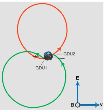
elec-tron orbits are distorted into cycloids. Their shape depends on whether the beam is injected with a component parallel or anti-parallel to the drift velocity. To be able to recognize both types of orbits simultaneously, EDI uses two guns and two detectors. Figure 1 shows examples of these two orbits in the plane perpendicular to B, which we refer to as the B⊥-plane.
For each gun, only one orbit-solution exists that connects it to the detector on the opposite side of the spacecraft. Know-ing the positions of the guns and the firKnow-ing directions that cause the beams to hit their detectors uniquely determines
GDU2
GDU1
E
B
v
Fig. 1. EDI principle of operation. For any combination of mag-netic field B and drift velocity Vd(assumed here to be induced by
an electric field E), only a single electron-trajectory exists that con-nects each gun with the detector on the opposite side of the space-craft. The two trajectories have different path lengths and thus dif-ferent times-of-flight. Note that for clarity the electron orbits are drawn for a very high drift velocity, Vd=1000 km s−1and an
un-realistically large magnetic field, B = 12 µT, implying an equally unrealistically large electric field of 12 V m−1, but a reasonable drift step of d = 3 m. For realistic magnetic fields, the gyro radius is much larger, e.g. 1065 m for a 100 nT field.
the drift velocity. This is the basis of the triangulation tech-nique, where one directly determines the “drift-step” vector d, which is the displacement of the electrons after a gyro time Tg:
d = VdTg (1)
The location in the B⊥-plane, from which electrons reach the
detector after one gyration, can be viewed as the “target” for the electron beams, as discussed in Quinn et al. (2001, this issue).
Note that for time-stationary conditions one gun-detector pair would suffice, because the satellite spin would rotate the gun into all positions sequentially. This is exactly what was done with the Electron Beam Experiment on Geos-2 (Melzner et al., 1978), which served as the proof-of-principle for the electron-drift technique In addition to being limited to spin-period resolution, the Geos instrument had a further limitation in that it could be operated only for small (< 18◦) angles between the ambient magnetic field and the spacecraft spin axis. EDI, with its fully steerable beams, can follow the target continuously regardless of magnetic field orientation.
As is evident from Fig. 1, the two orbits differ in their length, and thus in the electron travel times. The electrons
-40 -30 -20 -10 0 10 20 30 40 nT SC1, 24 Nov. 2000 1213:05-FGMx FGMy FGMz -40 -30 -20 -10 0 10 20 30 40 0 0.5 1 1.5 2 2.5 3 3.5 4 nT seconds Bx By Bz
Fig. 2. Synthesis of the FGM and STAFF magnetometer data that EDI receives on-board over the Inter-Experiment Link (IEL). The top panel shows the raw FGM data, received at 16 samples/s, which appears as a stair-case because it is sampled here every 4 ms. The bottom panel shows the combined (and rotated) data, which illus-trates the success of the synthesis method explained in the text. The plot uses the spacecraft convention with X along the spin axis. The sinusoidal variation in the Y - and Z-components is due to the space-craft spin. The plot was made from data stored in EDI’s scratch-RAM and dumped with the special BM3 telemetry mode that Clus-ter provides.
emitted with their velocity directed with a component paral-lel to Vd, i.e. away from the target, have a time of flight that
is shorter than Tg, while the electrons emitted towards the
target have a time of flight that is longer than Tg:
T1,2=Tg(1 ± Vd/Ve) , (2)
where Ve is the electron velocity. From Eq. (2) it follows
immediately that the difference between the two times-of-flight provides a measure of the drift velocity, Vd:
1T = T1−T2=2(Vd/Ve)Tg =2(d/Ve) , (3)
while their sum is twice the gyro time:
T1+T2=2 Tg. (4)
Noting that Tg =2π me/eB, this means that the
time-of-flight measurements allow B to be determined as well. Drift velocities encountered on a Cluster orbit typically range from a few km s−1 to less than 1000 km s−1, while the velocity of 1 keV electrons is 18 728 km s−1. Accord-ing to Eq. (3), this implies that 1T is only a small fraction of Tg, i.e. the drift introduces only a small variation in the
G. Paschmann et al.: EDI First Results 1275
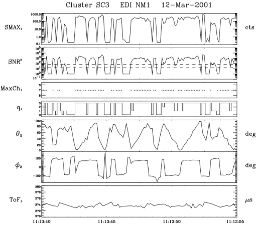
Fig. 3. EDI raw-data from Gun 2 and Detector 1 on SC 3 for a 15-second period on 12 March 2001, when the magnetic field strength was 100 nT. The top panel shows SMAX1, the maximum counts recorded (in 2 ms) in any of the 15 correlators in the Detector; the next panel
shows the square of the signal-to-noise ratio, SNR2, computed from the counts in the matched and unmatched correlators; the horizontal dashed lines in this panel indicate the thresholds for SNR2used by the on-board software to identify the beam (angle-track); the third panel shows MaxCh1, the correlator channel that received the maximum counts; when MaxCh1 = 7, time-track has been achieved; q1(fourth
panel) is a quality-status indicator explained in the text; the next two panels show 22and 82, the elevation and azimuth angles of the Gun 2 firing directions; ToF1(last panel) is the time-of-flight of the electrons from Gun 2 to Detector 1.
difference visible, Fig. 1 is drawn for unrealistically large magnetic and electric fields. The idea to use the difference in electron times-of-flight for drift velocity or electric field measurements is due to Tsuruda et al. (1985) and was first applied by the “boomerang” instrument on Geotail (Tsuruda et al., 1998). That instrument was, however, limited to one measurement per spin, and could not accommodate all mag-netic field orientations. EDI is the first instrument to combine the continuous triangulation and time-of-flight techniques, and, as already mentioned, can be operated for arbitrary mag-netic field orientations. EDI was first flown on the Equator-S mission and valuable information concerning operations and on-board software was gained, although limited by the short duration of the mission.
The triangulation and time-of-flight techniques comple-ment each other ideally. While triangulation naturally be-comes increasingly inaccurate if the target moves further and further away, the time-of-flight technique becomes more ac-curate because, according to Eq. (3), 1T increases with in-creasing drift steps, and thus becomes easier to measure. A first comparison of the two techniques on Equator-S was re-ported by Paschmann et al. (1999).
The electric field and gradients in the magnetic field both contribute to the drift velocity:
Vd =VE+V∇B, (5)
where, with W as the electron energy, the two drift velocities are defined as:
VE =(E × B)/B2, V∇B =(W/e)(B × ∇B)/B3.(6)
To separate VE and V∇B, two electron energies are
em-ployed. For W2=2W1one gets:
VE =2V1−V2, V∇B(W1) =V2−V1, (7) where V1and V2refer to the (total) drift velocities measured at W1and W2, respectively.
So far we have tacitly assumed that the beam electrons are detected after a single gyration. Electrons that have gy-rated N times will have a drift step and 1T that are N times larger. As we will see, electrons having gyrated several times (“multirunners”) are indeed observed. We will refer to N as the multirunner order.
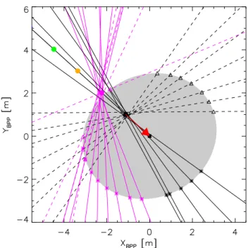
Fig. 4. Example of the triangulation analysis. The figure shows the spacecraft, the guns and the beam firing directions, all projected into the B⊥-plane, for a 4 s interval on 5 March 2001 (see Fig. 12).
Gun 1 and Gun 2 locations are indicated by asterisks and triangles, respectively, the beams emanating from these guns are shown as dashed and solid lines, respectively. The solid circles are placed at integer multiples of the drift step from the center of the space-craft, and are obtained from the best fit to all the beams in this in-terval. The (red) vector from the solid black circle to the center of the spacecraft is the drift step. The correct identification of the magenta-colored beams as double runners obviously has a profound effect on the drift step, identified by the black circle, which is the target for the single runners (black beams). No higher-order runners are present in this case. The drift step is 1.5 m in this case.
3 Implementation
3.1 Gun-detector characteristics
EDI consists of two gun-detector units (GDUs) and a con-troller unit. The GDUs are mounted on opposite sides of the spacecraft and have oppositely directed fields of view. The guns are capable of firing in any direction within more than a hemisphere (0–96◦polar angle) to accommodate arbitrary magnetic and electric field directions. Similarly, the detec-tors can detect beams coming from any selectable direction within more than a hemisphere (0–100◦polar angle).
Beams have an angular width of approximately 1◦at small polar emission angles, increasing to 4-by-1◦at large polar an-gles. Electron energies can be switched between 0.5 keV and 1.0 keV. Separate calibration tables for the two energies are used to convert beam firing directions into the corresponding deflection voltages.
The flux-density of the returning electrons is proportional to IbB3/E (except when the drift step is small). To
ac-commodate the large variations in B and E along the
Clus-ter orbit, the beam currents, Ib, can be changed over more
than two orders of magnitude (from 1 nA to several hundred nA). Beam currents are initialized based on the ambient mag-netic field strength and then varied automatically based on the tracking success.
Similarly, by using different combinations of high-voltages for the detector optics, a large variety of effective aperture areas, A, and geometric factors, G, can be realized. Aand G determine the sensitivity to beam and background electrons, respectively. By choosing the right combination of G and A, adequate signal and signal-to-noise-ratio (SNR) levels can be maintained over a wide range of field strengths and background electron fluxes. Tables of the optics voltages that achieve specific combinations of G and A are referred to as “Optics States”. The automatic Optics-State navigation is based on measured flux levels and magnetic field strength.
3.2 Time-of-flight measurements
In order to measure the electron times-of-flight, as well as to distinguish beam electrons from the background of ambient ectrons, the electron beams are amplitude-modulated with a pseudo-noise (PN) code. Nakamura et al. (1989) were the first to use a PN-code for (ion) drift measurements.
The EDI time-of-flight system has been described in ear-lier publications (Vaith et al., 1998; Paschmann et al., 1998, 1999). Briefly, a set of 15 correlators analyzes the phas-ing of the detector counts relative to the beam code. Be-fore beam acquisition has been achieved, all correlators will show the same counts (to within Poisson statistics) from the ambient electron background. Once the beam is acquired (“angle-track”), the correlator whose delay matches the elec-tron flight-time will have the maximum number of counts. A delay-lock-loop continuously shifts the code-phases of the correlators to keep the maximum centred in a specific chan-nel (“time-track”). By keeping track of the net change in code-phase, one obtains a measure of the changes in time-of-flight.
Commensurate with the number of correlators, EDI em-ploys primarily a 15-chip code. This way the signal is recorded in one of the correlators regardless of the actual time-of-flight. But because the accuracy is related to the chip-length, Tchip, the code-duration is kept short, much
shorter than Tg. The electron time-of-flight is therefore equal
to an integer number of code-lengths plus a fraction, of which only the fraction is measured by the correlators directly. However, by choosing a code-length equal to Tg/5 or Tg/10,
where Tgis estimated from the on-board FGM data, the
num-ber of complete wrap-arounds of the code can be recovered unambiguously. To track small time-of-flight variations, the code is shifted with a resolution of typically Tchip/32.
Sim-ulations of the correlator performance indicate that the ac-curacy of individual time-of-flight measurements is about Tchip/8. To account for the large variations in Tg along the
Cluster orbit, the code-length can be varied between approxi-mately 15 µs and 2 ms. A problem with the short code is that it does not discriminate against multi-runners. Regardless of
G. Paschmann et al.: EDI First Results 1277
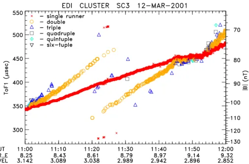
Fig. 5. Example of measured times-of-flight for Detector 1. The order of the multi-runners, identified by different symbols, has been determined by the method explained in the text. The scale on the right shows the magnetic field strength computed from the times-of-flight.
how many times the electrons have gyrated before hitting the detector, the signal will appear in one of the 15 correlators. We therefore have introduced a second, much longer code. It has 127 chips, and its length can exceed 4 Tg. By placing the
15 correlators at a time-delay near Tg, only single-runners
are detected (unless runners of order 5 or higher are present as well). As the increased chip-length implies lower accu-racy in time-of-flight measurements, the long code is only used in strong (> 100 nT) fields where multi-runners most frequently occur.
3.3 Beam acquisition and tracking
To find the beam directions that will hit the detector, EDI sweeps each beam in the plane perpendicular to B at a fixed angular rate (typically 0.2◦/ms) until a signal has been ac-quired by the detector. Once signal has been acac-quired, the beams are swept back and forth to stay on target. Beam detection is not determined from the changes in the count-rates directly, but from the square of the beam counts divided by the background counts from ambient electrons, i.e. from the square of the instantaneous signal-to-noise-ratio, SN R2. This quantity is computed from the counts recorded simulta-neously in the matched and unmatched correlator channels. If it exceeds a threshold, this is taken as evidence that the beam is returning to the detector. The thresholds for SN R2 are chosen dependent on background fluxes, and vary be-tween 35 and 200. These values have been selected after extended experimentation during commissioning, and rep-resent a compromise between getting false hits (induced by strong variations in background electron fluxes) and missing true beam hits. The basic software loop that controls EDI op-erations is executed every 4 ms. As the times when the beams hit their detectors are neither synchronized with the telemetry
nor equidistant, EDI does not have a fixed time-resolution.
3.4 On-board magnetic field data handling
EDI searches for the drift-step target in the plane perpen-dicular to B, and therefore needs information on the lo-cal instantaneous field as frequently as possible. Flux-gate magnetometer data are available on board over the inter-experiment-link (IEL) with the FGM instrument (Balogh et al., 1997). These data must first be time-tagged, because FGM sampling is not synchronized to the spacecraft clock, and then corrected for calibration angles, sensitivities, and offsets, and finally rotated by 6.5◦ to the spacecraft body axes. As the FGM data are available over the IEL only 16 times per second, the EDI controller constructs the field at higher frequencies using the analog signals from the three axes of the search-coil data provided by the STAFF instru-ment also over the IEL (Cornilleau-Wehrlin et al., 1997). To first order, the search coil signal is integrated and added pe-riodically to the FGM values, after rotations that account for the different coordinate systems of the two magnetometers. However, the frequency response of STAFF, as seen in Fig. 4 of Cornilleau-Wehrlin et al. (1997), differs from a pure dif-ferentiator in two respects. First, there is a high frequency roll-off above 40 Hz. EDI accepts this frequency basically as the limit at which it can track B. Second, there is a low-frequency cut-off that is inherent in the coil-pickup response. This reduces the signal primarily at the spacecraft spin fre-quency and is compensated by adding the properly phase-adjusted component at that frequency. Figure 2 shows the reconstructed signal for a time interval of about one spin pe-riod. The success of the reconstruction can be measured by the extent to which the discontinuities seen at the FGM up-date rate have been reduced.
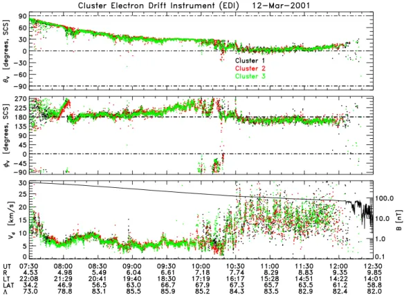
Fig. 6. EDI spin-resolution data from three spacecraft for the outbound pass on 12 March 2001, 07:30–12:30 UT. The top two panels show the elevation and azimuth angles of the drift velocity, 2vand 8v, in SCS coordinates. Because the flow is towards 180◦much of the time,
the scale for the azimuth is shown from −90◦to 270◦. The third panel shows the magnitude of the drift velocity, and, as a black line, the magnetic field magnitude measured by FGM on SC 1 for reference. The spacecraft position (in GSE) and invariant latitude, given along the bottom, are for SC 1. The data are plotted on the same scale for the three spacecraft and are placed at spin-center times, which are not identical because the spins of the Cluster spacecraft are not synchronized. As the green symbols (for SC 3) are plotted last, they are the only ones visible in regions of close agreement.
An accuracy of better than 0.5◦ in the direction of B is required because the width of the beam is about 1◦. Natu-rally, this poses stringent requirements on the calibration of the magnetometer data, as reconstructed by EDI from both the FGM and STAFF information, as described above. Er-rors of order 1 nT are of no concern to EDI if the total field is sufficiently large. However, for fields of 50 nT or less, beam-pointing errors can become larger than the beam width, causing loss of track if the error moves the beam off of the B⊥-plane. The EDI controller must maintain this accuracy
throughout four operational ranges of the FGM data, and this requires constant updates of the four calibration matrices, and four sets of offsets for each axis. As an overall con-straint on these numbers, the magnitude of the field is deter-mined by time-of-flight information whenever there are beam hits. As a starting point, the spin-axis offset is adjusted to be consistent with this magnitude. Furthermore, the plane per-pendicular to B is determined by the continual series of gun vectors that are successful. But as the beam-width is about one degree, and the tracking algorithm is able to keep the gun pointing only to within about 0.5 degrees of perpendicular to the varying B field, this information must be compiled statis-tically and used to correct the supplied calibration matrices
for accuracy in the EDI coordinate system. This process is iterated by ground processing, and then uplinked to the con-troller, to improve the success rate of beam hits.
3.5 Operations
The complex nature of the EDI operations and data process-ing has meant a long learnprocess-ing curve before the many con-trol parameters, beam-recognition algorithms, and magne-tometer calibrations had been adjusted sufficiently well that the instrument began to operate successfully under a wide range of ambient conditions. More than 15 patches to the onboard software have been uploaded so far. Still, when the magnetic field gets really low, and/or the background electron fluxes get high, tracking becomes difficult. Low B magnitudes require high beam currents to overcome the beam divergence along large gyro orbits, and to get suffi-cient signal-to-background ratio. But large beam currents, in conjunction with the beam-modulation and -coding lead to interference with the electric wave measurements by the WHISPER instrument (D´ecr´eau et al., 1997). Moreover, the smaller B gets, the higher the requirement for very precise on-board magnetometer calibrations. As mentioned in the previous section, improvements in these calibrations are
on-G. Paschmann et al.: EDI First Results 1279
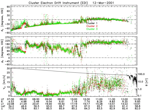
Fig. 7. The same data as in Fig. 6, except that the drift directions are now in GSE and the spacecraft motion has been corrected for.
going. Last but not least, rapid time-variations in magnetic and/or electric fields, as well as large fluxes of background fluxes can also cause loss of track.
4 Analysis 4.1 Data
EDI sends back the gun firing directions, detector count rates, measured times-of-flight, correlator settings, and some signal-quality information once every telemetry record, i.e. every 128 ms or 16 ms in nominal (NM) and burst (BM) telemetry, respectively. Additional auxiliary information (beam currents, optics states, control-loop parameter set-tings) is transmitted once every telemetry format (5.2 s). As EDI operates asynchronously, time-tags are added to every data record.
Figure 3 shows a 15-second period on 12 March 2001 that illustrates the character and quality of the raw EDI data when the magnetic field is fairly high, 100 nT in this case, and the flux of background electrons is very low. The spacecraft was transmitting in nominal (NM) mode, which means that an EDI data record is available once every 128 ms. In this ex-ample, which shows the data from Gun 2 and Detector 1 on SC 3, beam tracking was successful a large fraction of the time, as evidenced by the high detector counts in the top panel, but more significantly by the high (squared) signal-to-noise ratio (SNR) in the second panel, which is computed
from the contrast between matched and unmatched correlator channels. Levels of this quantity in excess of the threshold indicated by the lower dashed line mark the times when the beam has been acquired (angle-track). If the signal is kept in correlator number 7 (third panel), this indicates that time-track has been achieved as well. The occasional low signal-and SNR-levels indicate that the target has not been acquired, and only the ambient background electrons are detected. The 22and 82panels illustrate the rapid changes in gun firing directions that are being executed to track the moving target. Subsequent data processing is determined by the quality-status indicator q1 (fourth panel) that is transmitted in telemetry: q = 0 indicates that no beam-signal was acquired within the last 128 ms (16 ms in BM telemetry); q = 1 indi-cates angle-track, q = 2 indiindi-cates angle as well as time-track, q =3 in addition requires that the beam returns with an even higher SNR (upper dashed line in the second panel). The q = 0 data are useful because they provide the count rates from ambient electrons, as discussed in Quinn et al. (2001, this issue). The q = 1 data (angle-track only) have been ig-nored for the present analysis. In line with this selection, the times-of-flight in the bottom panel are shown only for those measurements that achieved time-track.
4.2 Analysis methods
From the information reported in telemetry, the beam direc-tions and gun posidirec-tions in spacecraft-sun (SCS) coordinates are computed, based on the Sun Reference Pulse (SRP). Our
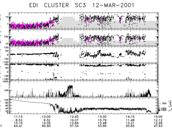
Fig. 8. Drift velocities on 12 March determined from the time-of-flight technique. The top panel shows the difference in the times-of-flight of the two beams, from which the magnitude of the drift velocity (second panel) is directly determined. There are two types of symbols in the top two panels (magenta-coloured circles and black crosses), which refer to the two different techniques to derive the 1ToFs, as explained in the text. Points in the grey area, which is based on Tchip/8 as the error of the individual measurements, and on the number of points within each 3-spin interval, are not significant. The next two panels show the drift direction. The fifth panel shows the counts (per 2 ms) received from ambient electron fluxes at 1 keV and 90◦pitch-angle, measured by EDI at the times when the beam was not detected. The bottom panel shows the spin-averaged magnetic field strength from FGM for reference. The scale on the right of that panel shows the electron gyro time computed from B.
standard analysis is then to select all beams within a certain time-interval, typically one spacecraft spin (4 s) and to per-form an automated determination of the drift step. For higher time resolution analysis, shorter intervals can be chosen (see Quinn et al., 2001, this issue).
4.2.1 Triangulation analysis
We have developed an analysis procedure that determines the drift step by searching for the target-point that minimizes an appropriate “cost-function”. For each grid-point in the B⊥plane, the cost-function is constructed by adding up the
(squared) angle-deviations of all beams in a chosen time in-terval from the direction to that grid-point. The present soft-ware allows selection of 1, 1/2 or 1/4 spin period as the anal-ysis interval. Each beam contribution to the cost-function is normalized by the (squared) error in the firing directions, which is a function of beam pointing direction and varies between 1◦ and 4◦. The grid-point with the smallest value of the cost-function is taken as the target. If a beam has been identified as a multi-runner of order N by the time-of-flight analysis (see Sect. 4.2.2), it is associated with a grid-point at N times the radial distance. When identification of
the order from the time-of-flight analysis is ambiguous, there is an alternate method where beams whose firing direction is closer to the direction towards the grid-point at N times the radial distance are counted as runners of order N . To speed up the search, the procedure uses a coarse grid to identify a restricted range in which the final search is performed with a much finer grid. The present software approximates the electron trajectories by circles whose radius is based on the magnetic field strength. An example of the drift step deter-mination using this method is shown in Fig. 4. The figure shows gun locations and firing directions for a 4 s (i.e. one spin) interval during which beams happened to be aimed at the single- and double-runner targets. Note that the construc-tion of the drift step from the firing direcconstruc-tions of the beams is for a virtual detector location at the center of the spacecraft. Thus the spacecraft is drawn at twice its actual dimensions, as explained in Quinn et al. (2001, this issue). The red vec-tor from the solid black circle to the center of the spacecraft is the drift step, determined, in the way described above, as the best fit to all the beams in the chosen interval. The figure emphasizes the importance of the correct identification of the multi-runners, in this case double-runners only. The example
G. Paschmann et al.: EDI First Results 1281
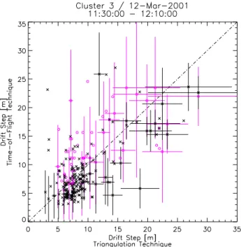
Fig. 9. Scatter plot of the drift speeds derived by the time-of-flight analysis (vertical axis) against those from the triangulation analysis (horizontal axis), for the interval 11:30 through 12:10 on 12 March 2001, on SC 3. The two types of symbols refer to the dif-ferent time-of-flight analysis methods, as in Fig. 8. Error bars are only shown for a fraction of the points so as not to clutter the figure.
is for a less than perfect focus to illustrate the power of the statistical approach of this analysis technique. An example of a much tighter focus is given in Quinn et al. (2001, this issue), Fig. 2. The analysis fails if the drift step and/or the magnetic field significantly vary within the chosen time interval. We can identify such cases by the variance in the magnetic field, by the quality of the fit (as measured by its reduced χ2), and by the angle or magnitude errors in the computed drift step. If those quantities exceed certain limits, no output is gener-ated. For the present paper, we have excluded data where the errors in drift step magnitude were larger than 30%, or the reduced χ2was larger than 20.
4.2.2 Time-of-flight analysis
The time-of-flight analysis serves three purposes. First and foremost, it is used to determine the drift velocity when the drift step becomes too large for the triangulation analysis. Second, it helps to identify multi-runners and thus can sup-port the triangulation analysis, and third, it is equivalent to a measurement of B. Deduction of the drift step (and the drift velocity) from analysis of the difference in the times-of-flight of the two beams (Eq. 3) is, in principle, straightforward.
If the drift step is large enough such that the firing direc-tions become nearly parallel, then one can easily group all the beams in the analysis interval (e.g. the spin period) into two oppositely directed sets. The set with the larger times-of-flight then must contain the beams directed towards the target, the other set those directed away from the target. This
assignment settles the drift direction, and the drift magnitude is then computed from the magnitude of the difference in the times-of-flight.
This simple scheme requires that conditions are stable over the analysis interval. If this is not the case, one should only use nearly simultaneous towards- and away-beam pairs for the analysis. But as we do not always have simultaneous hits from the two guns, we often have to resort to a method where we take the instantaneous difference between each measured time-of-flight and the gyro-time, Tg, computed from the
high-resolution magnetic field data from FGM. According to Eq. 2, the times-of-flight of the towards- and away-beams are symmetric around Tg, so that, in principle, either would
be sufficient to compute the magnitude of the drift. But be-cause the times-of-flight differ from Tgby a percent at most,
this scheme would work only if Tg were known precisely.
In practice, the Tgcomputed from the actual magnetic field
measurements, Tg,est, will not be properly centered, and we
therefore cannot apply this scheme directly. Instead, we aver-age the differences between any measured time-of-flight and the corresponding Tg,estseparately for the two sets of beams.
This way any fixed magnitude offset in Tg,estwill cancel out.
The set with the larger average is identified with the towards-beams, the other with the away-towards-beams, as above. The dif-ference between the two averages is then the quantity to use for 1T in Eq. 3. The identification of multirunners from the times-of-flight is illustrated in Fig. 5, which shows an exam-ple of the measured times-of-flight for Detector 1 for a one-hour interval on 12 March. The red x’s are the hits identified as single-runners. The other traces are from multi-runners, as identified in the legend. As described earlier, the PN-code is much shorter than the gyro time. In this particular case Tgvaries between 350 and 480 µs, while the code length
re-mains fixed at 114.4 µs. The electrons having gyrated twice have therefore an apparent increment in time-of-flight of Tg
modulo 114.4 µs relative to the single-runners. The same in-crement applies to each higher multiple. Inin-crements that are larger than half the code-length lead to apparent multirunner times-of-flight that are actually smaller, as seen in Fig. 5. Applying this simple rule one can then identify the multi-runner order N . Note that the slope of the multi-multi-runner traces is N times that of the single runners. Naturally, this method fails when Tgis itself a multiple of the code-length. In the
ex-ample at hand this condition occurs where the multi-runner traces intersect, near the beginning and end of the interval shown. As mentioned earlier, a by product of the EDI time-of-flight measurements is that they provide a precise determi-nation of the magnetic field magnitude. Data such as shown in Fig. 5 have been provided routinely to the FGM team to validate the spin-axis offsets in the FGM calibrations.
5 Results
In the following we present spin-resolution EDI data for three outbound passes when the apogee was located near local noon. During these orbits, EDI was not operated for
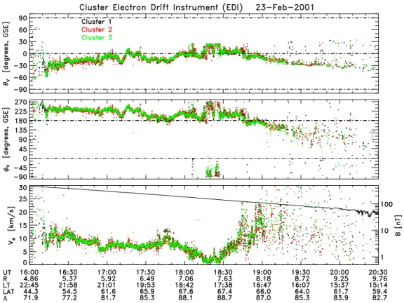
approxi-Fig. 10. Outbound pass on 23 February 2001, in the same format as approxi-Fig. 7, i.e. with the spacecraft velocity corrected for.
Fig. 11. Comparison of the drift velocities measured at 0.5 and 1.0 keV for the pass on 23 February, 16:30–19:00 UT. The plot shows the two components of the drift in the B⊥-plane, plus the magnitude. The magnitude of B is shown superimposed in the bottom panel.
G. Paschmann et al.: EDI First Results 1283
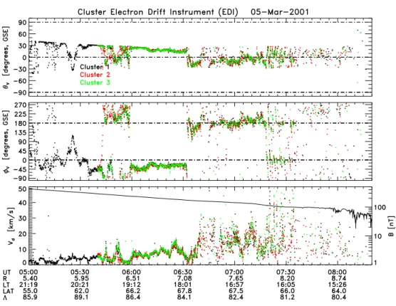
Fig. 12. Outbound pass on 5 March 2001 in the same format as Fig. 7. Note that until 05:40 only SC 1 data are available.
mately a 2-hour period centered on perigee. In addition, EDI was not operated on SC 4 during these orbits because of some intermittent overcurrent condition.
The EDI data are presented either as drift velocities or as electric fields, and in one of three coordinate systems. One is the spacecraft-sun (SCS) system, the second is the geocen-tric solar ecliptic (GSE) system, and the third is the B⊥-plane
system. The SCS system has its Z-axis along the spacecraft spin axis (directed nearly along the −ZGSE axis), and its X-axis directed sunward and is thus the system in which most Cluster instruments acquire their measurements. The GSE system has the advantage that it is an inertial system that al-lows to judge the drift direction in absolute terms. To be con-sistent with this inertial nature, we correct for the spacecraft velocity when showing data in GSE. The B⊥-plane (BPP)
system, on the other hand, is a natural system for EDI be-cause it emphasizes the fact that the measurements are two-dimensional in nature. It has the disadvantage that its axes change direction as B changes. The BPP-system has its X-axis directed towards the sun (more precisely X is in the plane containing B and the sun) and its Z-axis such that it has a positive ZGSEcomponent.
5.1 Outbound pass on 12 March 2001
Figure 6 shows the drift velocities, measured on space-crafts 1, 2 and 3, for the outbound pass on 12 March 2001 from 07:30 to 12:30 UT, obtained with the triangulation method (Sect. 4.2.1). The data start at 4.5 RE at 34◦
GSE-latitude, 73◦ invariant latitude, and 22 hours local time, i.e.
on magnetic field lines connected to the high-latitude edge of the nightside auroral oval. The orbit then crosses the north-ern polar cap and exits the magnetosphere at about 59◦ lati-tude at 12:10 UT, as determined from the sudden drop in B shown in the third panel. The drift velocities are presented in the SCS system and not corrected for spacecraft veloc-ity, to emphasize what is observed in the spacecraft system. The figure shows that there is very good overall agreement between the measurements on the three spacecraft, particu-larly regarding the drift directions. A proper interpretation of the drift velocities requires the data to be put into an iner-tial frame. Figure 7 therefore shows the same data, but now in GSE coordinates and corrected for the spacecraft motion. This correction means adding to the measured drift veloc-ity the perpendicular component of the spacecraft velocveloc-ity, because the motion of the spacecraft through the plasma im-plies a drift in the opposite sense. While the transition from SCS to GSE is simply a rotation, effectively flipping the signs of both angles, the correction for the spacecraft velocity has a dramatic effect, both in direction and magnitude. This is because in large parts of the pass the spacecraft velocity is of similar magnitude as the drift velocity, and furthermore both velocities are directed nearly opposite to each other some of the time. This means that the magnitude of the drift velocity can become very small after the correction, and its direction not only can become quite different, but also less well de-fined. This explains why the directions in Fig. 7 are much more variable much of the time than in Fig. 6. Note that the
Fig. 13. Drift velocity magnitude and phase in the gyro plane, for 07:15 to 07:30 on 5 March, demonstrating full 360◦rotations of the drift velocity vector.
triangular feature in the flow azimuth near 08:00 in Fig. 6 has now become a similarly looking feature in the drift magni-tude. As the drift velocity is, by definition, constrained to the B⊥-plane, its possible directions are restricted by the
mag-netic field orientation. This explains the sometimes clipped appearance of the angle-traces in this and the following fig-ures.
Figure 7 shows that after exiting the auroral flux tubes with their fairly high but variable convection velocities, the drift velocity stays low (< 5 km s−1) until 10:00 UT, with direc-tions ranging from anti-sunward to almost sunward. The dips in drift speed near 09:00 correspond to electric fields as low as 0.1 mV m−1, which highlights the sensitivity of the EDI measurements. Near 10:00, the convection speed suddenly becomes larger (10 − 20 km s−1) and highly variable, with equally variable directions, but the direction soon (at 10:30) settles on a stable, essentially anti-sunward direction (8v
near 180◦, 2vnear 0◦). There are only a few measurements
after 12:00 UT, i.e. when approaching the magnetopause, and their validity is questionable because of increasing time variations within the analysis interval.
Figure 8 shows the measurements for the same day from 11:00 UT up to the bow shock, which is crossed at 14:48 UT. In this case the drifts were determined from the 1ToFs, the difference in the measured times-of-flight of the two beams, shown in the top panel. There are two types of points (in this and the second panel). The open magenta-coloured circles were directly computed from the times-of-flight of
the two beams for those cases when they hit their detectors nearly simultaneously, within ±15 ms in this case. Those 1ToFs were then averaged over a three-spin interval that slides along one spin at a time. There are only few such points after 13:00 UT, because the number of hits was get-ting much smaller there and so did the likelihood of having near-simultaneous ones. The black crosses are also 3-spin averages, but were obtained by the other method described in Section 4.2.2, where the gyro-times estimated from the FGM data serve as intermediate reference. The agreement between the two sets of points is quite good.
The second panel shows the drift speeds computed from the 1ToFs according to Eq. 3, the third and fourth panels the drift directions. The drift directions are derived from the beam pointing directions and the time-of-flight analysis that involves the magnetic field as reference, thus the crosses. Only those directions are shown for which the drift magni-tude is significant, i.e. outside the grey area. In spite of this restriction, there are a few points left whose direction is op-posite to those of the others. These represent cases where the inferred 1ToFs apparently had the wrong sign.
Until about 12:00, the time-of-flight differences are of or-der 1 µs, compared to a code-chip length of 7.6 µs, and there-fore are just barely detectable. This explains the fairly large scatter in the derived drift speeds, whose magnitude is about 20 km s−1on average. Note that at this time the HIA sensor of the CIS instrument measures a bulk velocity component perpendicular to B of 20 km s−1, in good agreement with the
G. Paschmann et al.: EDI First Results 1285
EDI measurements (B. Klecker, private communication). The drift direction is well defined and stable, almost pre-cisely anti-sunward. At 12:05 the drift speed picks up and the direction becomes variable, until tracking stops at 12:20 because the magnetic field magnitude drops to 5 nT, indicat-ing the crossindicat-ing of the magnetopause. Such field strengths are prohibitively low for the EDI technique because of the B3 dependence of the flux that returns to the detector (see Sect. 3.1).
In the magnetosheath proper, i.e. after 13:00 UT, the 1ToFs rise to 10 µs on average, if one discounts the points in the grey area, corresponding to about 100 km s−1, and the convection is essentially anti-sunward, in good agreement with the perpendicular component of the bulk velocity mea-sured by HIA. But as the chip-length has risen to 30 µs, the accuracy is not much better than before 12:00. Furthermore, the magnetic field is now highly variable, and this introduces extra scatter.
Comparing the measured 1ToFs with the gyro times shown by the scale to the right of the bottom panel, it is apparent that the times-of-flight deviate by only 1% or less from the gyro times, which highlights the measurement problem. We are still working on optimizing the time-of-flight measurement accuracy, by reducing the chip-length, while at the same time maintaining adequate tracking ca-pability and avoiding the ambiguities inherent in the use of short code-lengths, discussed in Sect. 3.2.
Figure 8 also illustrates another aspect that affects EDI op-eration. The next to last panel shows the counts from am-bient electron fluxes at 1 keV energy and 90◦ pitch-angle, measured by EDI at the times when the beams are not de-tected (identified by the quality status q = 0). High fluxes are observed just outside the magnetopause and near the bow shock, in agreement with measurements by the PEACE in-strument (A. Fazakerley, private communication). To detect the beams in the presence of such high ambient fluxes would require very high beam currents. In spite of these limita-tions, Fig. 8 demonstrates that EDI is able to continuously track across the magnetosheath in magnetic fields that are as low as 30 nT and as variable as is typical for the magne-tosheath. EDI stops tracking at 14:40 UT, i.e. shortly be-fore the bow shock crossing, presumably because beam cur-rents were limited to about 100 nA at the time, and the fluxes of background electrons became high. Between 11:30 and 12:10 on this pass, the triangulation and time-of-flight anal-ysis methods have both provided results. In Fig. 9 we have plotted the drift steps obtained by the two methods against each other. Most of the points come from times before 12:00 where the drift steps are less than 10 m, and thus difficult for the time-of-flight technique to resolve. Nevertheless, the fig-ure shows that within the admittedly often large errors, there is reasonable agreement between the two techniques.
5.2 Outbound pass on 23 February 2001
Figure 10 shows an overview of the outbound pass on 23 February 2001 from 16:00 to 20:30 UT. At the beginning the
-4
-2
0
2
4
6
E
jin mV/m
-6
-4
-2
0
2
4
6
E
iin mV/m
Fig. 14. Hodogram of the electric field measured on SC 3 for the event from Fig. 13, illustrating the elliptical polarization of the os-cillations.
spacecraft are at 4.9 RE, 44◦GSE-latitude and 72◦invariant
latitude on auroral field lines, proceed across the northern po-lar cap and exit the magnetosphere near 20:20 UT, at 9.7 RE
and 60◦latitude in the afternoon sector. The orbit is similar to that for the 12 March pass, and so are many of the observed features, notably the variable drifts on auroral field lines, and the predominance of anti-sunward convection at typically 5-10 km s−1. Near 18:20 the magnitude of the drift velocity (after correction for the spacecraft velocity) becomes very low, less than 1 km s−1, corresponding to electric fields of only 0.1 mV m−1. The drift speed then picks up on average, but is highly variable. On approach to the magnetopause , i.e. after 19:20, there are occasional flips in drift direction by 180◦, from anti-sunward to sunward, which are not real and are probably due to variations occurring on spin-period time-scales. During part of this orbit, EDI on SC 2 was operated such that the electron energy was switched between 0.5 and 1.0 keV every second. Figure 11 shows that the drift veloc-ities measured at the two energies agree to within less than 0.5 km s−1most of the time, implying that the ∇B drift (see Eq. 7) was essentially zero, and the drift velocities measured at the two energies thus both represent the true E × B drift. More precisely, if one considers 0.5 km s−1to be the upper limit for the difference in drift velocities in this example, then according to Eq. 6, with B = 200 nT, one gets 10 000 km as the lower limit for the gradient scale length in the magnetic field at this time. If the gradient scale length had been larger, the drift velocities at the two energies would have become significantly different. The capability to separate the E × B and ∇B drifts is a unique feature of EDI and can be used to determine local magnetic field gradients if the induced drift
00:00 00:10 00:20 00:30 00:40 00:50 01:00 01:10 01:20 01:30 01:40 01:50 02:00 −15 −10 −5 0 5 10 E (mV/m)
Common Axis Comparison CL3
edi efw 00:00 00:10 00:20 00:30 00:40 00:50 01:00 01:10 01:20 01:30 01:40 01:50 02:00 −6 −4 −2 0 2 4 6 HR:MN of 7 Feb 2001 E (mV/m)
EDI Spin−Axis Electric Component
Fig. 15. Comparison of EDI and EFW electric fields. The top panel shows the component of E along the common axis defined in the text. The bottom panel shows the spin axis component measured by EDI.
is strong enough to compete with the electric field drift. So far we have not yet obtained measurements in regions where one expects the ∇B drift to contribute measurably to the total drift.
5.3 Outbound pass on 5 March 2001
An interesting event has been observed during the outbound pass on 5 March 2001. Figure 12 shows the drift velocities starting at 05:00 UT, when the spacecraft are near 5.4 RE
at 55◦latitude (86◦invariant latitude) and then proceed over the polar cap to the magnetopause, which is crossed after 08:00 UT. Until 06:30, drift speeds slowly increase from less than 1 to 10 km s−1, with highly variable directions, but over-all good agreement between the spacecraft. The low speeds just before 06:00 and after 06:30 correspond to electric fields of 0.1 mV m−1. There is a period (until about 07:15) when the drift velocities become highly variable in magnitude, but are predominantly anti-sunward. Starting at 07:18, large-amplitude oscillations are observed in direction and magni-tude, with periods near 1 to 1.5 min. Focusing on the interval 07:15 to 07:30 UT, and presenting the data as magnitude and phase of the drift velocity in the B⊥-plane, Fig. 13 shows
that the drift vector performs many full 360◦rotations dur-ing the event. The agreement between the three spacecraft
is remarkable, and there is no discernible time-displacement either, implying a structure that is homogeneous over a scale that exceeds the spacecraft separations, which range from 425 to 840 km. The hodogram of the equivalent electric field shown in Fig. 14 shows a very elliptical, left-handed polar-ization of the oscillations. The hodogram appears offset from the origin because of some net background drift velocity.
5.4 Comparison with EFW
As already stated in Sect. 1, the EDI and EFW instruments complement each other in that both directly or indirectly measure the electric field, but are subject to different kinds of limitations. It is therefore of great importance that the measurements are first compared under conditions when both should return valid electric field measurements. Figure 15 shows such a comparison on SC 3 on 7 February 2001. As EFW measures the field in the spin-plane, while the EDI measurements are in the B⊥-plane, the figure (top panel)
compares the electric fields along the common axis defined by the intersection of the two planes. The bottom panel shows the spin-axis component of the electric field that is measured by EDI but not by EFW, and that can often be a significant part of the total field. As the figure shows, the measurements along the common axis agree remarkably well
G. Paschmann et al.: EDI First Results 1287
in this case, for which that axis is almost transverse to the earth-sun line. We are presently studying some occasions, when the common axis is more nearly aligned with the earth-sun line, or when there are rapid excursions of the plasma density to very low values, where the agreement is usually not so good. The large electric fields observed in this case, which when mapped into the ionosphere are of the order of 100 mV m−1, correspond to the onset of a substorm on this date, as seen by EFW and EDI on spacecrafts 1, 2 and 3. This will be the subject of a later publication.
6 Summary
In this paper we have presented three polar passes that demonstrate that EDI is able to make precise drift velocity measurements under a wide range of conditions, which in-clude the low and variable magnetic and electric fields in the magnetosheath . Drift velocities as low as 1 km s−1are observed, corresponding to electric fields of 0.1 mV m−1. An outstanding feature in these observations is the quasi-periodic electric field rotationsobserved on 5 March 2001 over the polar cap on the dayside at 81◦invariant latitude. A key advantage of the EDI technique is that the beam probes the ambient electric field at a distance of some kilometers from the spacecraft, and therefore essentially outside the lat-ter’s influence. Furthermore, the analysis is essentially ge-ometric in nature and thus the accuracy can be quite high. And last but not least, EDI always measures the entire drift velocity, and thus the total transverse electric field, includ-ing any component along the spacecraft spin axis, while the double-probe instrument on Cluster (EFW) measures only in the spin-plane. On the other hand, EDI beam tracking will be disrupted in very low magnetic fields, large fluxes of ambi-ent electrons, and by very rapid changes in magnetic and/or electric fields. Thus EDI and EFW complement each other nicely. Comparisons with EFW are turning out to be very promising, as the remarkable agreement in the example pre-sented in this paper demonstrates. Comparisons with the per-pendicular component of the plasma bulk velocity measured by the CIS instrument have also started.
A unique feature of EDI is its capability to separate the E × B and ∇B drifts that we have demonstrated with one example in this paper (where the ∇B drift happened to be essentially zero). This capability could be used to determine magnetic field gradients over the distance of the electron gyro radius, thus complementing the technique to infer the gradi-ents over a much larger scale from the magnetic field mea-surements on the four spacecraft.
Acknowledgement. The authors would like to thank the many peo-ple who have made the EDI experiment possible through 15 years of development, testing, and operations: B. Austin, B. Briggs, J. Chan, M. Chutter, R. Frenzel, W. G¨obel, J. Googins, D. Hallmark, W. Isaac, G. King, S. Longworth, K. Lynch, R. Maheu, F. Melzner, J. Needell, U. Pagel, P. Parigger, D. Simpson, W. St¨oberl, J. St¨ocker, K. Strickler, and C. Young. We owe great thanks to the payload team at Dornier, in particular Roland Nord, and to the entire project
team at ESTEC. We acknowledge the excellent operations support by the project scientists at ESTEC, Philippe Escoubet and Michael Fehringer, and by the team at ESOC, in particular Sandro Matussi and Michael Schmidt. EDI could not be operated without the accu-rate on-board magnetometer data from FGM and STAFF, and we are grateful to Andre Balogh and Nicole Cornilleau-Wehrlin and their teams for the cooperative support they have provided. We thank Forrest Mozer and the EFW team for their efforts on the EDI-EFW comparisons. Joshua Semeter gave advice concerning the analysis technique. We dedicate this paper to the memory of Norbert Sck-opke, who contributed so much to the success and spirit of Cluster and EDI, but did not live to see the result. This work was supported by DLR through grants FKZ: 50OC89043 and FKZ: 50OC9705, and by NASA through grants NAS5-30744 and NAG5-9960.
The Editor in Chief thanks D. Fontaine and F. Lefeuvre for their help in evaluating this paper.
References
Balogh, A., Dunlop, M. W., Cowley, S. W. H., Southwood, D. J., Thomlinson, J. G., Glassmeier, K. H., Musmann, G., L¨uhr, H., Buchert,S., Acu˜na, M. H., Fairfield, D. H., Slavin, J. A., Riedler, W., Schwingenschuh, K., and Kivelson, M. G.: The Cluster Mag-netic Field Investigation, Space Sci. Rev., 79, 65–191, 1997. Cornilleau-Wehrlin, N., Chauveau, P., Louis, S., Meyer, A., Nappa,
J. M., Perraut, S., Rezeau, L., Robert, P., Roux, A., De Villedary, C., De Conchy, Y., Friel, L., Harvey, C. C., Hubert, D., Lacombe, C., Manning, R., Wouters, F., Lefeuvre, F., Parrot, M., Pincon, J. L., Poirier, B., Kofmann, W., and Louarn, Ph.: The Cluster Spatio-Temporal Analysis of Field Fluctuations (STAFF) Exper-iment, Space Sci. Rev., 79, 107–136, 1997.
D´ecr´eau, P. M. E., Fergeau, P., Krasnosel’skhikh, V., L´eveque, M., Martin, Ph., Randriamboarison, O., Sen´e, F. X., Trotignon, J. G., Canu, P., and M¨ogensen, P. B.: WHISPER, a resonance sounder and wave analyser: performances and perspectives for the Clus-ter mission, Space Sci. Rev., 79, 157–193, 1997.
Gustafsson, G., Bostr¨om, R., Holback, B., Holmgrn, G., Lund-gren, A., Mozer, F. S., Pankow, D., Harvey, P., Berg. P., Ulrich, R., Pedersen, A., Schmidt, R., Butler, A., Franssen, A. W. C., Klinge, D., F¨althammar, C.-G., Lindqvist, P.-A., Christenson, S., Holtet, J., Lybekk, B., Sten, T. A., Tanskanen, P., Lappalainen, K., and Wygant, J.: The electric field and wave experiment for the Cluster mission, Space Sci. Rev., 79, 137–156, 1997. Melzner, F., Metzner, G., and Antrack, D.: The Geos electron beam
experiment, Space Sci. Rev., 4, 45, 1978.
Nakamura, M., Hayakawa, H., and Tsuruda, K.: Electric field mea-surement in the ionosphere using the time-of-flight technique, J. Geophys. Res., 94, 5283–5291, 1989.
Paschmann, G., Melzner, F., Frenzel, R., Vaith, H., Parigger, P., Pagel, U., Bauer, O. H., Haerendel, G., Baumjohann, W., Sck-opke, N., Torbert, R. B., Briggs, B., Chan, J., Lynch, K., Morey, K., Quinn, J. M., Simpson, D., Young, C., McIlwain, C. E., Fil-lius, W., Kerr, S. S., Maheu, R., and Whipple, E. C.: The Electron Drift Instrument for Cluster, Space Sci. Rev., 79, 233–269, 1997. Paschmann, G., McIlwain, C. E., Quinn, J. M., Torbert, R. B., and Whipple, E. C.: in: The electron drift technique for measuring electric and magnetic fields, (Eds) Pfaff, R. F., Borovsky, J. E. and Young, D. T., Measurement Techniques in Space Plasmas: Fields, 29–38, Geophysical Monograph 103, AGU, Washington, D. C., 1998.
Paschmann, G., Sckopke, N., Vaith, H., Quinn, J. M., Bauer, O. H., Baumjohann, W., Fillius, W., Haerendel, G., Kerr, S. S., Klet-zing, C. A., Lynch, K., McIlwain, C. E., Torbert, R. B., and Whipple, E. C.: EDI electron time-of-flight measurements on Equator-S, Ann. Geophysicae, 17, 1513–1520, 1999.
Quinn, J. M., Paschmann, G., Sckopke, N., Jordanova, V. K., Vaith, H., Bauer, O. H., Baumjohann, W., Fillius, W., Haerendel, G., Kerr, S. S., Kletzing, C. A., Lynch, K., McIlwain, C. E., Torbert, R. B., and Whipple, E. C.: EDI convection measurements at 5– 6 REin the post-midnight region, Ann. Geophysicae, 17, 1503– 1512, 1999.
Quinn, J. M., Paschmann, G., Torbert, R. B., Vaith, H., McIlwain, C. E., Haerendel, G., Bauer, O. H., Bauer, T., Baumjohann, W., Fillius, W., F¨orster, M., Frey, S., Georgescu, E., Kerr, S. S., Klet-zing, C. A., Matsui, H., Puhl-Quinn, P., and Whipple, E. C.: Cluster EDI convection measurements across the high-latitude plasmasheet boundary at midnight, Ann. Geophysicae, 19, this
issue, 2001.
Tsuruda, K., Hayakawa, H., and Nakamura, M.: in: Science Objec-tives of the Geotail Mission, (Ed) Nishida, A., 234, ISAS, Tokyo, 1985.
Tsuruda, K., Hayakawa, H., and Nakamura, M.: Electric field mea-surements in the magnetosphere by the electron beam boomerang technique, in: Measurement Techniques in Space Plasmas: Fields, (Eds) Pfaff, R. F., Borovsky, J. E., and Young, D. T., 39–45, Geophysical Monograph 103, AGU, Washington, D. C. , 1998.
Vaith, H., Frenzel, R., Paschmann, G., and Melzner, F.: Electron gyro time measurement technique for determining electric and magnetic fields, in: Measurement Techniques in Space Plasmas: Fields, (Eds) Pfaff, R. F., Borovsky, J. E., and Young, D. T., 47–52, Geophysical Monograph 103, AGU, Washington, D. C., 1998.