Effect of circumferential groove casing treatment parameters on axial compressor flow range

Effect of Circumferential Groove Casing Treatment

Parameters on Axial Compressor Flow Range

by

Brian K. Hanley

B.S. Mechanical Engineering, California Institute of Technology, 2006

Submitted to the Department of Aeronautics and Astronautics in partial

fulfillment of the requirements for the degree of

ARCHNE8

Master of Science in Aeronautics and Astronautics

at the

MASSACHUSETTS INSTITUTE OF TECHNOLOGY

_{JUN 2 3 2010}

June 2010

LIBRARIES

C Massachusetts Institute of Technology 2010. All rights reserved.

Autho

Department of Aeronautics and Astronautics

-

May

21,

2010

Certified by:

Choon S. Tan

Senior Research Engineer

Thesis Supervisor

Certified by:

Edward M. Greitzer

H. N. Slater Professor of Aeronautics and Astronautics

Thesis Supervisor

Accepted by:

Eytan H. Modiano

Associate Professor o Aeronautics and Astronautics

Chair, Committee on Graduate Students

Effect of Circumferential Groove Casing Treatment Parameters on

Axial Compressor Flow Range

by

Brian K. Hanley

Submitted to the Department of Aeronautics and Astronautics on May 21, 2010 in partial fulfillment of the

requirements for the degree of

Master of Science in Aeronautics and Astronautics

Abstract

The impact on compressor flow range of circumferential casing grooves of varying groove depth, groove axial location, and groove axial extent is assessed against that of a smooth casing wall using computational experiments. The computed results show that maximum range improvement is obtained for a groove depth of approximately a tip clearance and of an axial width of approximately 0.175 axial chord (approximately the near stall tip clearance vortex core size for the smoothwall compressor examined). It was found that for a groove of specified depth and axial width there are two axial locations, one at approximately 0.15 axial chord and one at approximately 0.6 axial chord from the rotor blade leading edge, to position the groove for maximum flow range improvement; this result is in accord with recent experimental observations.

In addition, a method of extracting body forces is used to show that the force is finite at the blade tip and non-vanishing in the tip clearance.

Thesis Supervisor: Choon S. Tan Title: Senior Research Engineer

Thesis Supervisor: Edward M. Greitzer

Acknowledgements

I would like to thank Professor Greitzer and Dr. Tan for all of the assistance they have provided during this project. I would also like to express my appreciation for the advice and insight of Dr. Sean Nolan, which was considerably useful in my

understanding of the project.

Additionally, David Car, Tomoki Kawakubo, and Jon Kerner all provided invaluable advice that helped me make sure I was running my calculations correctly. I would also like to thank Jeff Defoe, who supplied immeasurable technical assistance both for general systems use in the lab and for pointers on getting my computations to run the way I needed them to.

I would also like to thank GTL for providing me with the computational tools I used to complete the research for this project.

Table of Contents

1 Introduction and Background

1.1 Body Force Representation of Compressor Blade-row

1.2 Casing Treatment 1.3 Contributions

1.4 Organization of Thesis 2 Technical Approach

2.1 Assessment of Body Force Representation of Compressor Rotor with Tip Clearance

2.2 Assessment of Circumferential Groove Casing Treatment on Compressor Operating Range

2.2.1 Mesh Generation for Casing Grooves with Varying Depth, Axial Location, and Axial Extent

2.2.2 Compressor Rotor Pressure Rise Characteristic

3 Compressor Rotor Blade Body Force Distribution in the Endwall Flow

Region

3.1 Pressure Distribution on the Rotor Blade Surface

3.2 Body Force Distribution in the Rotor Blade Region

3.3 Body Force Calculation in the Tip Gap

3.4 Summary

4 Effect of Casing Groove Depth on Compressor Stall Margin 4.1 Sizing and Placement of Casing Groove

4.2 Stall Margin Improvement

14 14 15 17 18 19 19 22 22 25 27 27 33 36 39 40 40 41

4.3 Effect of Variation in Depth of Casing Grooves on Endwall Streamwise 44 Momentum

4.4 Effect of Variation in Depth of Casing Grooves on Tip Clearance 49 Vortex Location

4.5 Dependence of Results on Mesh Resolution 53

4.6 Summary 55

5 _{Effect of Casing Groove Axial Location on Compressor Stall Margin 56}

5.1 Sizing and Placement of Casing Groove 56

5.2 Stall Margin Improvement 56

5.3 Effect of Variation in Axial Location of Casing Grooves on Endwall 59 Streamwise Momentum

5.4 Effect of Variation in Axial Location of Casing Grooves on Tip 62

Clearance Vortex Location

5.5 Summary ₆₃

6 Effect of Casing Groove Axial Extent on Compressor Stall Margin 64

6.1 Sizing and Placement of Casing Groove 64

6.2 Stall Margin Improvement 64

6.3 Effect of Variation in Axial Extent of Casing Grooves on Endwall 66

Streamwise Momentum

6.4 Effect of Variation in Axial Extent of Casing Grooves on Tip Clearance 69

Vortex Location

6.5 Summary ₇₀

7.1 Summary and Conclusions 71

7.2 Future Work 72

A Calculation of Body Force Distribution 73

List of Figures

1-1 Sketch of generic circumferential casing grooves 15

2-1 Meshed domain used for computing flow for body force extraction 20

2-2 A representative computed speedline for rotor used in assessing body 21 force representation

2-3 Meshed domain for circumferential casing groove 0.15 chord deep 23

2-4 Meshed domain with a circumferential casing groove sized and located 24 by the blade tip

2-5 Speedline for a circumferential casing groove 0.15 chord deep 25

3-1 Static pressure distribution at 0.8 span 28

3-2A Static pressure distribution at 0.88 span 29

3-2B Static pressure distribution at 0.9 span 29

3-2C Static pressure distribution at 0.92 span 30

3-2D Static pressure distribution at 0.94 span 30

3-2E Static pressure distribution at 0.96 span 31

3-2F Static pressure distribution at 0.98 span 31

3-2G Static pressure distribution at 0.99 span 32

3-2H Static pressure distribution at 0.999 span 32

3-3A Normalized axial body force in rotor blade region 34

3-3B Normalized tangential body force in rotor blade region 34 3-4A Spanwise distribution of normalized axial body force per unit span 35

3-5A Color plot of normalized axial body force in the blade region on the 37

upper 20% of the span and in the tip clearance

3-5B Color plot of normalized tangential body force in the blade region on 37

the upper 20% of the span and in the tip clearance

3-6A Spanwise distribution of normalized axial body force per unit span on 38

the upper 20% of the span and in the tip clearance gap

3-6B Spanwise distribution of normalized tangential body force per unit span 38

on the upper 20% of the span and in the tip clearance gap

4-1 Example casing groove geometry 41

4-2 Speedlines for 0.15 chord deep groove and smoothwall 42 4-3 Variation in stall margin improvement with depth of casing groove of 44

fixed axial location and axial extent, compared to Nolan [5]

4-4 Radial transport of streamwise momentum at the blade tip with 45 variations in groove depth

4-5 Radial transport of streamwise momentum into the groove from the 47 endwall region with variations in groove depth

4-6 Total radial transport of streamwise momentum out of the endwall 48 region with variations in groove depth

4-7A Comparison of tip clearance vortex location for smoothwall and for 49 groove with a depth of 0.01 chord

4-7B Comparison of tip clearance vortex location for smoothwall and for 50

4-7C Comparison of tip clearance vortex location for smoothwall and for 50

groove with a depth of 0.04 chord

4-7D Comparison of tip clearance vortex location for smoothwall and for 51 groove with a depth of 0.075 chord

4-7E Comparison of tip clearance vortex location for smoothwall and for 51 groove with a depth of 0.12 chord

4-7F Comparison of tip clearance vortex location for smoothwall and for 52

groove with a depth of 0.15 chord

4-8 Comparison of tip clearance vortex location for smoothwall and 54 different levels of mesh refinement

5-1 Variation in stall margin improvement with axial location of casing 57

groove of fixed depth and axial extent

5-2 Stall margin for cases of varied groove axial location and groove depth 58

as measured by Houghton and Day [6]

5-3 Radial transport of streamwise momentum at the blade tip with 59 variations in groove axial location

5-4 Radial transport of streamwise momentum into the groove from the 60

endwall region with variations in groove axial location

5-5 Total radial transport of streamwise momentum out of the endwall 61

region with variations in groove axial location

6-1 Variation in stall margin improvement with axial extent of casing 65

6-2 Radial transport of streamwise momentum at the blade tip with 66

variations in groove axial extent

6-3 Radial transport of streamwise momentum into the groove from the 67

endwall region with variations in groove axial extent

6-4 Total radial transport of streamwise momentum out of the endwall 68

region with variations in groove axial extent

List of Tables

3-1 Area of static pressure distributions for constant span 33

4-1 Tip clearance vortex location for various casing groove depths 52 4-2 Examination of mesh resolution with respect to stall margin 53

improvement

4-3 Examination of mesh resolution with respect to radial transport of 54

streamwise momentum at the blade tip

5-1 Tip clearance vortex location for various casing groove axial locations 62

Nomenclature

Aaxi,= axial area of computational cell wall

Aradial = radial area of computational cell wall

fx = axial blade force

fo

F, = extracted tangential body force

F, = extracted radial body force

Forcelade = body force on the blade

Leompressor = characteristic length of the compressor

P = static pressure

P,= total pressure

P = reference pressure

r, = radius of blade tip

rh = radius of hub s = blade pitch u. = friction velocity u = axial velocity U0 = tangential velocity ur = radial velocity u= streamwise velocity

U = blade tip speed

Uwheel =midspan blade speed

y' =non-dimensional distance from the wall (

)

Volumecell = computational cell volume

A= metal blockage - r(0₂ - 1), where subscripts 1 and 2 denote one rotor blade and

S

nearest adjacent rotor blade in the same stage

p = density

-r = tip clearance

v = kinematic viscosity

D= total-to-static pressure coefficient

Chapter 1 Introduction and Background

Axial compressor instability is a major limiting factor in the design and use of gas turbine engines. Axial compressor instabilities can occur as stall and surge (Hill and Peterson, [1]). It is of engineering interest to have means of predicting axial compressor

instability and to have design methodologies that can delay the onset of axial compressor instabilities. A method of predicting axial compressor instability through examination of body forces in the axial compressor rotor blade region is currently being developed [2, 3, 4]. The use of casing treatment is a design methodology that can be used to delay the onset of axial compressor instabilities. Circumferential casing grooves provide a design methodology that can be assessed using steady-state calculations.

1.1 Body Force Representation of Compressor Blade-row

The first objective of this thesis is to assess the body force at the tip of an axial compressor and in the tip clearance gap.

Previous research (e.g. Kiwada [2], Reichstein [3], and Kerner [4]) has examined the use of a blade-row-by-blade-row body force representation of an axial compressor in a computational model as a means for assessing compressor instability. Kiwada

developed a method for extracting body forces for representing compressor blade-row from a three-dimensional flow field computed using a computational fluid dynamics (CFD) solver. While Kiwada, Reichstein, and Kerner have examined the general trends

in body force representation of the blade-row with compressor operating points, they have not specifically focused on what constitutes an adequate body force representation that reflects the effects of tip clearance flow. This is of import as it is known that compressor tip clearance has a significant impact on compressor instability onset. An objective of this thesis is to assess the variation of body force representation of a compressor rotor in the rotor tip gap.

1.2 Casing Treatment

The second objective of this thesis is to assess quantitatively the variation in stall margin improvement with groove depth, groove axial location, and groove axial extent.

FIG. 1-1 Sketch of generic circumferential casing grooves

- Casing treatment is one method used to extend axial compressor operable flow

range. Typically, casing treatment comprises one or more slots or grooves in the section of the casing above the tip of the blade. In this thesis, the effects of sizing and location of

a single circumferential casing groove is assessed on compressor performance (operable range and pressure rise).

The effect of variation of depth and axial location of single circumferential groove casing treatment on the flow range of an axial compressor was examined by Nolan [5] and by Houghton and Day [6]. Nolan found that shallow grooves increase the flow range of the compressor and that the increase with groove depth asymptotically approaches a value corresponding to a groove depth on the order of one tip clearance. However the initial high rate of increase in stall margin with depth is such that it calls for further investigation. Further, Nolan showed that for a circumferential groove positioned near the tip clearance vortex core, significant improvement in compressor flow range is obtained over that for the associated smoothwall axial compressor.

Houghton and Day [6] performed a series of experiments to assess the effect of varying the axial location of a single circumferential groove on the flow range of an axial compressor. Their experimental measurements for a casing treatment groove located at varying axial locations showed two maxima in stall margin improvement over a

smoothwall compressor, one for a groove located at 0.1 axial chord downstream of the leading edge of the rotor blade and one for a groove located at 0.5 axial chord

downstream of the leading edge of the rotor blade. They also carried out experiments to assess the effect of casing groove depth on stall margin improvement; their measurements show that that a shallower groove leads to a reduced improvement in stall margin for all axial locations.

As a method for understanding the mechanism by which circumferential casing grooves improve the flow range of an axial compressor, Shabbir and Adamczyk [7] examined the relation between the radial transport of axial momentum in the tip clearance region to the shear and normal pressures on the casing and casing treatment. Shabbir and Adamczyk examined cases with four and five circumferential casing grooves and

analyzed the effectiveness of the four and five groove cases with respect to the changes in momentum and pressure. They found that the mechanism for improvement was related to the radial transport of axial momentum.

1.3 Contributions

The key findings in this thesis are as follows:

1) A method of extracting body forces is use to show body force of a rotor blade

is finite at blade tip and non-vanishing in the tip clearance gap.

2) The estimated operable flow range increases with groove depth approaching an eventual value corresponding to that for a groove depth of one tip

clearance; the rate of increase in the estimated flow range with groove depth is less than that reported in reference [5].

3) There are two maxima in the estimated improvement over the smooth casing

compressor: one with the groove located at 0.15 axial chord and the other at 0.6 axial chord downstream of the rotor leading edge. This is a first-of-a-kind

The computed results are in accord with the recent experimental measurements by Houghton and Day [6].

4) The improvement in estimated compressor operable flow range is positive for grooves of axial extent less than 0.4 axial chord; for groove axial extent larger than 0.4 axial chord, the estimated useful flow range decreases. The

implication is that for groove axial extent larger than 0.4 axial chord, the compressor corresponds to that of a smoothwall compressor with increased tip clearance.

1.4 Organization of Thesis

This thesis is organized as follows. In chapter 2, the technical approach used in the computation of the results in the subsequent chapters is described. Chapter 3 describes the body force representation of an axial compressor and demonstrates that in the body force representation of a rotor blade row, the body force is finite at the blade tip and is non-vanishing in the tip clearance gap. Chapter 4 describes the effect of variation of circumferential casing groove depth on estimated flow range. Chapter 5 describes the effect of variation of circumferential casing groove axial location on estimated flow range. Chapter 6 describes the effect of variation of circumferential casing groove axial extent on the estimated flow range. Finally, the findings and conclusions are presented in chapter 7; suggestions for future research on circumferential casing groove are also presented in chapter 7.

Chapter 2 Technical Approach

This chapter outlines the methods used to calculate the flow fields for assessing body force distribution in the rotor blade tip region and for determining the effect of

circumferential casing groove geometry variations on compressor flow range.

2.1 Assessment of Body Force Representation of Compressor Rotor with Tip Clearance

For determining the body force distribution that represents the action of axial compressor blade with tip gap on the flow, a Reynolds average Navier-Stokes

computational fluid dynamics (CFD) solver has been used. The compressor rotor chosen for assessing the tip clearance effect on compressor rotor representation by body force was a representative low Mach number rotor with a 0.03 span tip clearance. The solver used is the commercial CFD package FLUENT.

FIG. 2-1 shows the meshing of the flow domain using GAMBIT. It comprised

two sections, a first section for the tip clearance and a second section for all flow outside of the tip clearance. Due to constraints imposed by the blade geometry, the tip clearance section required the use of an unstructured mesh. The second section used a structured mesh where cell density increases near the walled boundaries of the flow domain to resolve boundary layer flows. Specifically, cell density increases in the radial direction near the hub and casing boundaries, in the pitchwise direction near the pressure side and

suction side of the blade, and in the axial direction near the leading edge and trailing edge of the blade. The increased cell density near the boundary regions allowed for acceptable y+ values as required by the turbulence modeling, which used the realizable k-epsilon

model* [8,9].

I

Tip

FIG. 2-1 Meshed domain used for computing flow for body force extraction

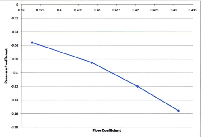
The steady-state pressure rise characteristics have been obtained by implementing calculations of three-dimensional flow at operating points from design to "numerical" stall. The operating point was selected by setting the exit static pressure and inlet stagnation pressure. Swirl was specified at the inlet boundary to simulate an inlet guide vanes. A radial equilibrium condition was applied at the exit boundary to set the exit static pressure profile. A representative pressure rise characteristic is given in FIG. 2-2.

* _{The use of the realizable k-epsilon model was suggested by Kawakubo to achieve a more accurate loss}

level for the axial compressor used.

The operating point corresponding to "numerical" stall is the operating point beyond which the mass flow continuously decreases for the specified exit pressure and a steady-state solution is unattainable. Assessment of the body force representation of the

compressor rotor is done using the computed operating point nearest to the compressor design point.

FIG. 2-2 A representative computed speedline for rotor used in assessing body force representation 0..19 0395 0-4 0405 OA OA15 OA2 0425 043 0.435 -0.02 -0.04 -0.06 -01 0. -0.12 -0.14 -0.16 -018 ewC.efficimt

2.2 Assessment of Circumferential Groove Casing Treatment on Compressor

Operating Range

Groove depth, groove axial location, and groove axial extent were varied to enable the determination of the parametric trend on the operable range and change in performance. Circumferential casing grooves are assessed solving the standard k-epsilon model for the E3 rotor B, with a 0.03 chord tip clearance.

2.2.1 Mesh Generation for Casing Grooves with Varying Depth, Axial Location, and Axial Extent

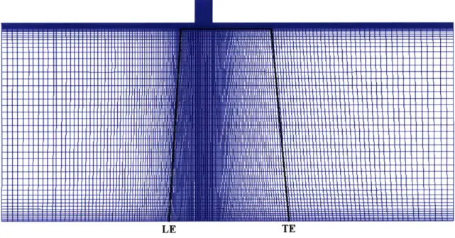
The flow domain for cases of casing grooves with varying depth was meshed in three sections using the commercial mesh generation package Pointwise/GridGen: a tip clearance section, a casing groove section, and a section for the main flow. All three sections use a structured mesh with cell density increasing near the solid walled boundaries of the mesh. Cell density increases in the radial direction near the hub and casing boundaries, in the pitchwise direction near the pressure side and suction side of the blade, and in the axial direction near the leading edge and trailing edge of the blade as well as the leading edge and trailing edge of the casing groove. The increased cell

density near the boundary regions allowed for acceptable y+ values (30 to 300) as required by the turbulence modeling. FIG. 2-3 shows a representative meshing of this flow domain, including a 0.15 chord deep casing groove.

LE TE

FIG. 2-3 Meshed domain for circumferential casing groove 0.15 chord deep

Casing groove depth was varied to create different geometries by removing cells from the top of the groove section mesh. This procedure facilitated the determination of the change in the steady state flow field as a result of the different casing groove depths. Further the compressor flow path with a smooth casing wall can readily be generated by removing the groove section mesh entirely.

A higher resolution mesh for the compressor rotor flow path was also generated to

evaluate the effect of mesh size on the computed flow. This refined mesh was created to have twice the cell density in the axial dimension, radial dimension, and pitchwise dimension of the baseline mesh.

A third mesh was generated for varying casing groove axial location and axial

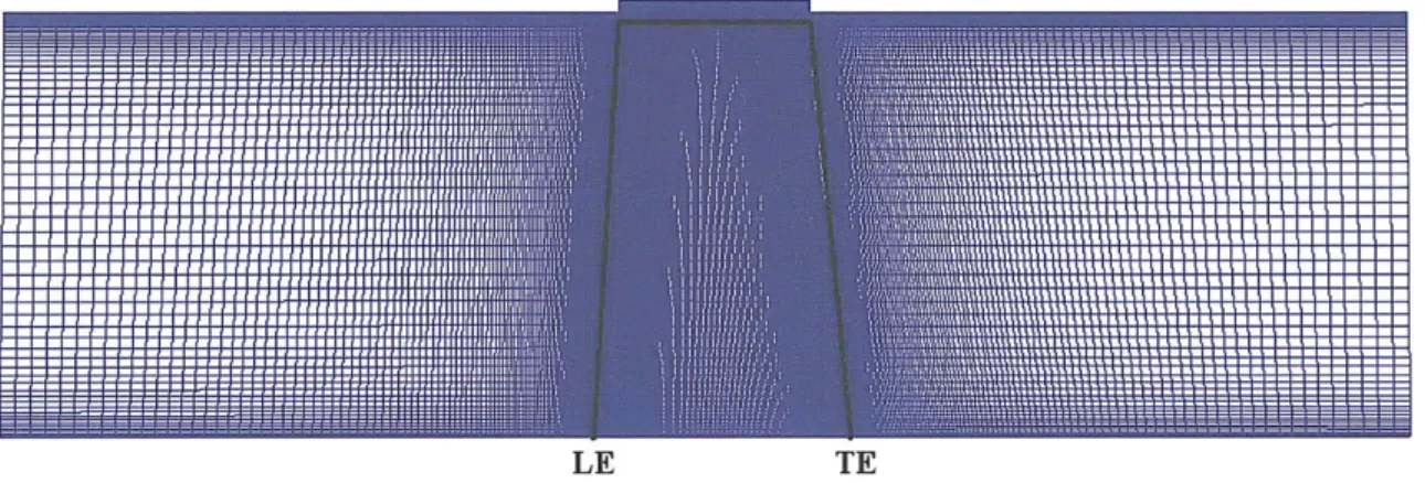
meshed in three sections. All three sections use a structured mesh with cell density increasing near the walled boundaries of the mesh. In the case of this third mesh, the groove is defined at a constant depth, has an axial location where the groove leading edge is inline with the leading edge of the blade tip, and has axial extent matching the axial extent of the blade tip. FIG. 2-4 shows a meshing of the flow domain as described above for the third mesh.

LE TE

FIG. 2-4 Meshed domain with a circumferential casing groove sized and located by the blade tip

The mesh for a casing groove with a different axial location or a different axial extent can readily be obtained by the selective removal of cells from the groove section mesh. For example, for a groove with specified axial extent and axial location, the corresponding mesh was generated by removing the cells upstream of the leading edge and downstream of the trailing edge of the groove to meet the specification. Likewise, the corresponding mesh for a smooth casing wall can be obtained by simply removing the groove section mesh entirely.

2.2.2 Compressor Rotor Pressure Rise Characteristic

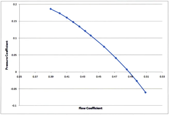
As described in section 2.1, the compressor characteristic has been obtained by implementing steady-state calculation of three-dimensional flow at several operating points from design to numerical stall. A representative computed performance

characteristic is given in FIG. 2-5.

now coaft

FIG. 2-5 Speedline for a circumferential casing groove 0.15 chord deep

An estimate of tall margin improvement can be obtained by comparing the numerical stall coefficient of a smoothwall compressor to the numerical stall of a compressor with a circumferential casing groove. As in equation 2.1, the stall margin

015 0.1 0.05 0 0 -0.05 0.37 0.39 0.41 0A3 0.45 0A7 4 0.51 0.53 ... ... .

improvement represents the flow range extension of the compressor with a circumferential groove casing treatment over a smoothwall compressor.

Stall Margin Improvement = groove,stall - smooth,stall (2.1) smooth,stall

Chapter 3 Compressor Rotor Blade Body Force Distribution in the

Endwall Flow Region

In this chapter, the computed flow field in an axial compressor rotor is used to assess the body force representation of the rotor blade in the endwall flow region.

Examination of pressure distribution on the rotor blade as well as body force distribution in the rotor blade region shows that the computed body force is finite in the endwall region.

3.1 Pressure Distribution on the Rotor Blade Surface

An indicator of blade force on the rotor blade of a compressor is the static pressure distribution on the suction side and pressure side of the rotor blade; the

integrated pressure difference across the blade provides a measure of the magnitude of the pressure force. An assessment of the pressure forces on the blade may provide a trend indicating the magnitude of the body force on the blade as the tip gap is approached.

0.6 0.4 0.2 S0-C) : -0.2 00.4 -05 -0.6- -0.8-0 0.1 0.2 0.3 0.4 0.5 0.6 0.7 0.8 0.9 1 Axial Position, LE (x = 0), TE (x = 1)

FIG. 3-1 Static pressure distribution at 0.8 span

The static pressure distribution across the blade at 0.8 span is shown in FIG. 3-1. The pressure distribution shown in FIG. 3-1 is expressed in terms of a pressure

coefficient defined in equation 3.1.

Static Pressure Coefficient = ref (3.1)

Static pressure distributions at various spanwise locations approaching the blade tip are shown in FIG. 3-2A to FIG. 3-2H. At 0.999 span, there is still a pressure

difference between the pressure side and the suction side of the blade, indicating a finite force on the blade close to the tip.

U 0.4 -0.2 0 CD :3-0.2 - -0.40.6 -0.8 --a 0.1 0.2 0.3 0.4 0.5 0.6 0.7 0.8 0.9 Axial Position, LE (x =0), TE (x = 1)

FIG. 3-2A Static pressure distribution at 0.88 span

0.G 0.4-0.2 -S0 -i-0.2 -- .- 0.4--05 -0.6- -0.8--1 ' 0 0.1 0.2 0.3 0.4 0.5 0.6 0.7 0.8 0.9 Axial Position, LE (x 0). TE (x = 1)

0.6 0.4 -0.2 0 -0 S-0.2--0 -0. --1 0 0.1 0.2 0.3 0.4 0.5 0.6 0.7 0.8 0.9 Axial Position, LE (x = 0), TE (x = 1)

FIG. 3-2C Static pressure distribution at 0.92 span

0.4 0.2 0--0.2 a S-0.4-- -0.6--0.8 ---1 1 1 1 1 1 1 1 1 1 0 0.1 0.2 0.3 0.4 0.5 0.6 0.7 0.8 0.9 Axial Position, LE (x 0), TE (x = 1)

0.4 - 0.2- 00.2 --0.4 EO -0.6 -0.8 U 0.1 0.2 0.3 0.4 0.5 0.6 0.7 0.8 0.9 1 Axial Position, LE (x =0), TE (x = 1)

FIG. 3-2E Static pressure distribution at 0.96 span

0.G 0.4 4E 0.2 -0 0.4 -Axial Position, LE (x = 0), TE (x = 1)

0 C-)

-0.2

0 0.1 0.2 0.3 0.4 0.5 0.6 0.7 0.8 0.9 1 Axial Position, LE (x = 0), TE (x = 1)

FIG. 3-2G Static pressure distribution at 0.99 span 0.6 -0.4 -0.6 -0.8-0 0.1 0.2 0.3 0.4 0.6 0.6 0.7 0.8 0.9 1 Axial Position, LE (x = 0), TE (x = 1)

FIG. 3-2H Static pressure distribution at 0.999 span

The change in the blade force can be defined in terms of the integrated pressure side and suction side pressure distributions. Table 3-1 gives the area bounded by the pressure side and suction side pressure distributions at spanwise locations corresponding to those from FIG. 3-1 and 3-2A to 3-2H.

Table 3-1 Area of static pressure distributions for constant span

Spanwise Location Area/Blade Force

0.8 Span 0.2150 0.88 Span 0.2269 0.9 Span 0.2330 0.92 Span 0.2434 0.94 Span 0.2591 0.96 Span 0.2853 0.98 Span 0.3143 0.99 Span 0.3166 0.999 Span 0.1288

As shown in Table 3-1, the area bounded by the pressure side and suction side distributions increases when traversing up the span from 0.8 span to 0.98 span. The area at 0.99 span is slightly higher than the area at 0.98 span. The area at 0.999 span is lower than the area for the other spans shown, but still substantial, specifically 60% of the value of the area at 0.8 span and 40% of the value of the area at 0.99 span. This implies there is a non-zero pressure force at the blade tip.

3.2 Body Force Distribution in the Rotor Blade Region

The body force distribution in the blade region can be calculated from steady state, three-dimensional flow using the procedure described in Appendix A. The calculated body force distribution is shown in FIG. 3-3A and 3-3B. The procedure from Appendix A generates blade force per unit mass which is then normalized to be non-dimensional by

1 U2

2 wheel to yield the normalized axial force shown in FIG. 3-3A and the normalized Lcompressor

tangential force shown in FIG. 3-3B. It is difficult to infer a useful trend in the body force near the tip from FIG. 3-3A and 3-3B except that it is non-vanishing in the tip

clearance region. However it would be useful to assess the spanwise variation of axially integrated body force from the leading edge to the trailing edge, particularly in the tip gap.

0.9 0.8 S.7 0S.6~E 07 0.5 -c 0.4 0.3 0.2 0.1 0 0.2 0.4 0.6 0.8

Axial Position (span lengths)

3. 3-3A Normalized axial body force in rotor bl

0.9 0.8 a-0.7 co 0.6 0.5 a 0.4 0.3 0.2 0.1 0 0.2 0.4 0.6 0.8

Axial Position (span lengths)

3-3B Normalized tangential body force in rotor

0 10 10 20 ade region 10 10 20 -30 blade region FI FIG.

C

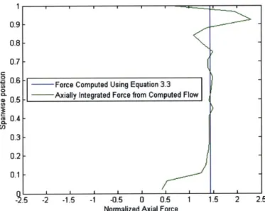
0.6 - - _{Force Computed Using Equation 3.3}

0.5 - Axially Integrated Force from Computed Flow

CL_0.4 En 0.3- 0.2- 0.1-5 -2 -1.5 -1 -0.5 0 0.5 1 15 2 2.5 Normalized Axial Force

FIG. 3-4A Spanwise distribution of normalized axial body force per unit span 1

0.9-0.8

--- Force Computed Using Equation 3.4 0.7 - Axially Integrated Force from Computed Flow 0.6 0.5 0.4 0.3 -0.2 0.1 2- 0 2 4 6 8 10

Normalized Tangential Force

FIG. 3-4B Spanwise distribution of normalized tangential body force per unit span

Spanwise distributions of axially integrated body force from the leading edge to the trailing edge are shown in FIG. 3-4A and 3-4B. FIG. 3-4A and 3-4B also show the axial and tangential body forces calculated from using equations 3.3 and 3.4 respectively (Dixon [10]). In equations 3.3 and 3.4, subscripts of 1 and 2 denote the flow variable at the rotor inlet and rotor exit respectively.

f,

f

=

psu2

u,

₂

(3.3)

Ux Ux/

In the hub region, both the axial and tangential forces are relatively small. By 0.1 span, both the axial and tangential forces are approximately equal to the forces computed using equation 3.2 and 3.3. The axial force in the tip region varies in magnitude from approximately 0.8 span to the blade tip where the value is non-zero, indicating that the axial body force can be non-vanishing beyond the tip of the blade. Likewise, the

tangential force varies in magnitude from approximately 0.8 span to the blade tip with a finite value indicating that the tangential body force can be non-zero beyond the tip of the blade as well.

3.3 Body Force Calculation in the Tip Gap

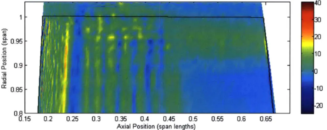
The procedure used in chapter 3.2 to calculate body force distribution in the blade region can be adapted to calculate body forces in the tip gap. Looking at the tip region specifically in FIG. 3-5A and 3-5B, there are regions of non-vanishing body forces in the tip clearance gap.

0 .O0.95 A: 10 CL 0.9 0.85 10 20 0.8 0.15 0.2 0.25 0.3 0.35 0.4 0.45 0.5 0.55 0.6 0.65 Axial Position (span lengths)

FIG. 3-5A Color plot of normalized axial body force in the blade region on the upper 20% of the span and in the tip clearance gap

0 (OFo.9 10 o~0.9 cc -10 E 0.85 20 15 0.2 0.25 0.3 0.35 0.4 0.45 0.5 0.55 0.6 0.65

Axial Position (span lengths)

FIG. 3-5B Color plot of normalized tangential body force in the blade region on the upper 20% of the span and in the tip clearance gap

The spanwise variation of axially integrated body forces in the tip region is shown in FIG. 3-6A and 3-6B. In the tip region, axial force decreases from the tip to the casing. The tangential force also decreases from the tip to the casing and is greater than zero.

Apart from the oscillation in the tip clearance region which is the result of errors in interpolation when using the body force extraction procedure*, the trend in FIG. 3-6A and 3-6B shows non-zero forces in the tip clearance.

-2 -1.5 -1 -0.5 0 0.5 Normalized Axial Force

1 1.5 2 2.5

FIG. 3-6A Spanwise distribution of normalized axial body force per unit span on the upper 20% of the span and in the tip clearance gap

-2 0 2 4 6 8 10

Normalized Tangential Force

FIG. 3-6B Spanwise distribution of normalized tangential body force per unit span on the upper 20% of the span and in the tip clearance gap

* This is a consequence of using Kiwada's extraction method with a CFD package other than Denton's

TBLOCK solver [2].

0.951

0.85

3.4 Summary

Examination of the static pressure distribution on the blade and the body force acting on the blade indicates that body force acting at the tip of the blade is non-zero. Additionally, the trend in both the static pressure distribution and the body force

Chapter 4 Effect of Casing Groove Depth on Compressor Stall Margin

In this chapter the effect of circumferential casing groove depth on compressor stall margin is assessed. The effect of circumferential casing grooves on the radial transport of streamwise momentum and the location of the tip clearance vortex core is also determined.

4.1 Sizing and Placement of Casing Groove

An assessment of the effect of casing groove depth on stall margin was carried out. The selection of axial location and axial extent for the groove was based on guidelines provided by Nolan [5]; Nolan used the estimated tip clearance vortex core size and

position to size the casing groove axial extent and to select the axial location of a single casing groove for the E3 rotor. The leading edge of the casing groove is located at 0.2 axial chord downstream from the leading edge of the blade and the casing groove has an axial extent of 0.175 axial chord. Nolan investigated the effect of varying the depth of a single casing groove at this location from 0.0015 to 0.03 chord. The mesh created in accordance with the description in section 2.2.1 is used to calculate the flow for groove depths up to 0.15 chord. This configuration is shown in FIG. 4-1. The results are assessed against those of a corresponding smoothwall configuration as presented in the next section.

Side View

Flow Direction

Top View

Giroove

FIG. 4-1 Example casing groove geometry

4.2 Stall Margin Improvement

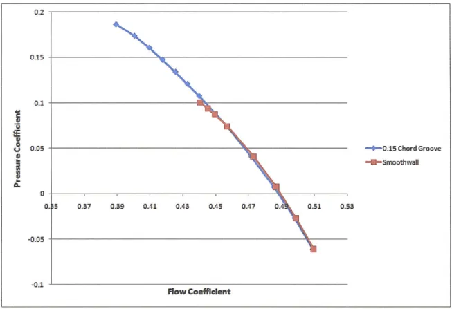
All the grooved cases showed increases in both flow range and peak pressure rise

over the smooth wall case. FIG. 4-2 shows the increases of flow range and pressure rise of a 0.15 chord deep groove compared to the smooth wall case.

0.15 .1 0.05 -- 0.15 Chord Groove 6 --WSmoothwall 3 t. 0 0. 5 0.37 0.39 0.41 0.43 0.45 0.47 0.4 0.51 0.53 -0.05 -0.1 Flow Coefficient

FIG. 4-2 Speedlines for 0.15 chord deep groove and smoothwall

The pressure coefficient used is total-to-static pressure rise as expressed in

equation 4.1. The flow coefficient is mass-averaged axial velocity at the inlet normalized by the rotor blade tip speed as expressed in equation 4.2.

Pressure Coefficient T = P2 1 (4.1)

uu

Flow Coefficient (D = Ux (4.2)

The improvement in flow range over the smooth wall case can be expressed in terms of stall margin improvement. Stall margin improvement is calculated as in equation 2.1. FIG. 4-3 shows the effect of different casing groove depths on the stall margin improvement as computed for this thesis and by Nolan [5]. The computed results

for this thesis show stall margin improvement increases to a maximum (approximately 12% change in stalling flow coefficient compared to the smoothwall case) for a groove with a depth of 0.04 chord. Stall margin improvement then dips slightly between groove

depths of 0.04 chord depth and 0.15 chord depth, with a low at 0.12 chord depth. The initial rate of increase in stall margin improvement of Nolan's results [5] shows that by a depth of 0.003 chord there is an improvement in stall margin of approximately 10%. The computed results of this thesis show a much more gradual increase in stall margin

improvement (stall margin improvement of 10% is reached for a groove depth between 0.02 chord and 0.04 chord).

FIG. 4-3 Variation in stall margin improvement with depth of casing groove of fixed axial location and axial extent, compared to Nolan [5]

4.3 Effect of Variation in Depth of Casing Grooves on Endwall Streamwise Momentum

Nolan [5] argued that reduction of radial transport of streamwise momentum out of the endwall region would lead to an improvement of stall margin and peak pressure rise relative to that for a smoothwall case. Nolan hypothesized that a circumferential

casing groove positively affected the radial transport of streamwise momentum and was a major contributing factor to the mechanism by which circumferential casing grooves

improve stall margin. The normalized radial transport of streamwise momentum can be computed using expression 4.3 [5] where the integration in the numerator extends over a single blade passage from the leading edge to the trailing edge of the blade on a radial

0.18 0.16 0.14 0.12 0.1 0.06 0.04 0.02 0 0.08 -4-Computed Resufts -- Nolan's Results [51 0.12 0.14 0.16 0.02 0.04 0.06 0.08 0.1 r..e .Ighe/chard ....... ... ... .... I I ... ... --- - - - - . . .. .... .. I . . .. ..........0 0 0 ................ ........ = -VAa " 1b L

-surface at the blade tip. The computed values for various groove depths are shown in FIG. 4-4. The negative quantities of normalized radial transport of streamwise

momentum in FIG. 4-4 represent loss of streamwise momentum from the endwall region. Values of normalized radial transport greater than the baseline smoothwall case represent

an expected benefit to the flow field of the compressor.

JUrUsdA tp * (', ~''.) _(4.3) Forcebi,.e e 0 I 4i 0.02 0.04 0.06 0.08 0.1 0-12 0.14 0.16 -0.1 E -0.2 E 0 -0.3 -0.4 -4-Grooved rotor -U-SoothmWal Basline 0-C -0--0.7 -0.8

FIG. 4-4 Radial transport of streamwise momentum at the blade tip with variations in groove depth

The results in FIG. 4-4 show that the beneficial radial transport of streamwise momentum at the tip is only marginally greater for a groove depth of 0.02 chord

compared to the smoothwall case. For all other depths, the radial transport of streamwise momentum at the tip is less than that for the smoothwall case. This seems to indicate that the mechanism for improvement for circumferential casing grooves may not necessarily be associated with a reduction in radial transport of streamwise momentum out of the tip location.

Evaluation of the radial transport of streamwise momentum from the endwall region into the groove may provide further insight, as streamwise momentum could

transfer from the groove to the endwall flow to counter the loss at the tip location. FIG.

4-5 shows the radial transport of streamwise momentum from the endwall region to the

groove for varying groove depths as calculated using expression 4.4 where the limits of integration in the numerator are defined by the radial surface of the groove entrance. Positive normalized transport of streamwise momentum in FIG. 4-5 represents transport

of streamwise momentum from the endwall region into the groove; such a transfer of momentum constitutes a loss of streamwise momentum from the endwall region.

0.035 0.03 E

I

FIG. 4-5 Radial transport of streamwise momentum into the groove from the endwall region with variations in groove depth

JJ

uUrdA

groove __r,-r_

Forceblade

(4.4)

In FIG. 4-5, the trend initially looks similar to the change in stall margin with groove depth in FIG. 4-3. However, the direction of radial transport is into the groove, which increases the streamwise momentum flux lost from the endwall region. FIG. 4-6 shows the total radial transport of streamwise momentum out of the endwall region defined in equation 4.5. Beneficial total radial transport of streamwise momentum out of the endwall region is expected to be represented by values of total radial transport of

streamwise momentum greater than the smoothwall baseline total radial transport of streamwise momentum. 0 0.02 0.04 0.06 0.08 0.1 0.12 0.14 0.16 -0.2 E U* -0.3 E E -J -0.4 -0-Grooved rotor 0

A-.5 -- Smoothwall Baseline

0 I.

M

-0.7

Groove Depth/Chord

FIG. 4-6 Total radial transport of streamwise momentum out of the endwall region with variations in groove depth

JJPUrUsdA JJPUrUsdA

Total Radial Transport = *ip - * (r - rh groove *rt - h (4.5)

Forceblade r Forceblade T

FIG. 4-6 shows the total radial transport as slightly lower (0.004) for a 0.01 chord

deep casing groove than when compared to the smoothwall case. The total radial

transport out of the endwall region then asymptotically decreases until a groove depth of 0.075 chord. This appears to suggest that the mechanism by which circumferential

casing grooves improve stall margin and pressure rise may not be linked to a reduction in the radial transport of streamwise momentum out of the endwall region as hypothesized by Nolan [5].

4.4 Effect of Variation in Depth of Casing Grooves on Tip Clearance Vortex Location

Nolan [5] also hypothesized that the tip clearance vortex shifted downstream as a result of the presence of a circumferential casing groove. A simplified method of

viewing the location of the tip clearance is to use the pitchwise averaged radial velocity at the blade tip [5]. FIG. 4-7A through 4-7F show comparisons between the radial velocity

distribution of the smoothwall case and cases with various groove depths.

Smoothwall

0.06 - -0.01 Chord Deep Groove

0 Smoothwall Tip Clearance Vortex Location

0.04 - 0 0.01 Chord Deep Groove Tip Clearance Vortex Location 0.02 - 0> 0.02 CE0.04 --0.06 --0.08 --0.1 1II 0 0.1 0.2 0.3 0.4 0.5 0.6 0.7 0.8 0.9 1 Axial Location, LE (x = 0). TE (x = 1)

FIG. 4-7A Comparison of tip clearance vortex location for smoothwall and for groove with a depth of 0.01 chord

0.06 Smoothwall

0.02 Chord Deep Groove

0 Smoothwall Tip Clearance Vortex Location

0.04 _{0 0.02 Chord Deep Groove Tip Clearance Vortex Location} 0.02 0 0--0 > -0.02 -0.04 -0.06 -0.08 0 0.1 0.2 0.3 0.4 0.5 0.6 0.7 0.8 0.9 -Axial Location, LE (x = 0), TE (x = 1)

FIG. 4-7B Comparison of tip clearance vortex location for smoothwall and for groove with a depth of 0.02 chord

Smoothwall

0.06 - - _{0.04 Chord Deep Groove}

o Smoothwall Tip Clearance Vortex Location

0.04- 0 0.04 Chord Deep Groove Tip Clearance Vortex Location 0.02 0-> -0.02 -0.04 -0.06- -0.08--0.1 0 0.1 0.2 0.3 0.4 0.6 0.6 0.7 0.8 0.9 Axial Location, LE (x = 0), TE (x = 1)

FIG. 4-7C Comparison of tip clearance vortex location for smoothwall and for groove with a depth of 0.04 chord

Smoothwall

0.075 Chord Deep Groove

o Smoothwall Tip Clearance Vortex Location

0 0.075 Chord Deep Groove Tip Clearance Vortex Location

-0.1 0.2 0.3 0.4 0.5 0.6 0.7 Axial Location, LE (x = 0), TE (x = 1)

0.8 0.9 1

FIG. 4-7D Comparison of tip clearance vortex location for smoothwall with a depth of 0.075 chord

and for groove

0.06 0.04 0.02 0 > -0.04 -0.06 -0.08 -0.1 0 Smoothwall

0.12 Chord Deep Groove

o Smoothwall Tip Clearance Vortex Location

0 0.12 Chord Deep Groove Tip Clearance Vortex Location

0.1 0.2 0.3 0.4 0.5 0.6 0.7 0.8 Axial Location, LE (x = 0), TE (x = 1)

0.9 1

FIG. 4-7E Comparison of tip clearance vortex location for smoothwall and for groove with a depth of 0.12 chord

0.06 0.04 0.02 -0.02 -0.04 -0.06 -0.08. -0.1 -0 I I I I I I I I I --

I j I a I I I a I

0.06 - Smoothwall

0.15 Chord Deep Groove

0 Smoothwall Tip Clearance Vortex Location

0.04 0 _{0.15 Chord Deep Groove Tip Clearance Vortex Location} 0.02 - 0-> -0.02 c' -0.04 --0.06 --0.08 -0 0.1 0.2 0.3 0.4 0.5 0.6 0.7 0.8 0.9 1 Axial Location, LE (x = 0), TE (x = 1)

FIG. 4-7F Comparison of tip clearance vortex location for smoothwall and for groove with a depth of 0.15 chord

Examining the radial velocity distributions in FIG. 4-7A to 4-7F show that for each casing groove depth the tip clearance vortex center shifted downstream compared to the smoothwall case. Table 4-1 gives the estimated location of tip clearance vortex locations for various groove depths. As the depth of a casing groove increases, the estimated tip clearance vortex location shifts downstream; however the quantity by which the tip clearance vortex shifts downstream does not correlate to the change in stall margin.

Table 4-1 Tip clearance vortex location for various casing groove depths

Depth of groove Location of vortex in fraction of axial chord

Smoothwall 0.41 0.01 chord deep 0.455 0.02 chord deep 0.465 0.04 chord deep 0.475 0.075 chord deep 0.485 0.12 chord deep 0.495 0.15 chord deep 0.495

4.5 Dependence of Results on Mesh Resolution

As mentioned in section 2.2.1, two meshes were used to evaluate the effect of circumferential casing grooves of varying depth. The meshes were compared for a casing groove depth of 0.02 chord. Table 4-2 shows the stall margin improvement calculated for the standard mesh as discussed in section 4.1 and 4.2 and the stall margin improvement calculated for the refined mesh.

Table 4-2 Examination of mesh resolution with respect to stall margin improvement Stall Margin Improvement

Standard Mesh .0901

Refined Mesh .1067

Difference .0166

The difference in stall margin improvement as a result of mesh refinement

is .0166. This value is smaller than the effect of variation of groove depth as discussed in this chapter and smaller than the effect of groove axial location and axial extent as

discussed in chapters 5 and 6 respectively. For further examination of the difference between the standard grid and the refined grid, pitchwise average radial velocity at the blade tip for the smoothwall case, the standard and refined grid cases is shown in FIG.

- Smoothwall

- _{0.12 Chord Deep Groove, Standard Mesh} 0.12 Chord Deep Groove, Refined Mesh 0.06 0 Smoothwall Tip Clearance Vortex Location

0 0.12 Chord Deep Groove Tip Clearance Vortex Location, Standard Mesh 0.04 _{0.12 Chord Deep Groove Tip Clearance}

Vortex Location, Refined Mesh 0.02 - 0-> -0.02 S-0.04 -0.06 --0.08 --0.1 1 1 0 0.1 0.2 0.3 0.4 0.5 0.6 0.7 0.8 0.9 1 Axial Location, LE (x = 0), TE (x = 1)

FIG. 4-8 Comparison of tip clearance vortex location for smoothwall and different levels of mesh refinement

The pitchwise averaged velocity is similar for both the standard and refined mesh. In both cases, the vortex core is shifted downstream by approximately 0.07 axial chord. There are two main differences. The radial velocity from 0.3 to 0.45 axial chord is higher for the refined case and the radial velocity from 0.6 to 0.9 axial chord is higher for the refined case. These results suggest that the radial transport of streamwise momentum at the blade tip may be less for the refined mesh than for the standard mesh. The values of radial transport of streamwise momentum at the blade tip for the standard mesh and the refined mesh are detailed in table 4-3.

Table 4-3 Examination of mesh resolution with respect to radial transport of streamwise momentum at the blade tip

Case Radial Transport

Standard Mesh -0.709

Refined Mesh -0.661

While the refined mesh shows increased stall margin improvement, the change is approximately 2%, small compared to the improvement due to the presence of the groove (4% to 12%). The radial velocity is similar for the two cases. The results suggest that the additional computational resources/time required to compute solutions for the refined mesh is not required.

4.6 Summary

The circumferential groove with a groove depth of 0.04 chord depth yielded the maximum improvement in stall margin. This groove depth is approximately one tip clearance in size. The rate of increase in stall margin improvement with groove depth from zero (smoothwall) to 0.04 chord is less than that reported by Nolan [5].

The results also indicate that a link between stall margin improvement and the change in radial transport of streamwise momentum out of the endwall region (or the change in tip clearance vortex location) cannot be established.

Chapter

5

Effect of Casing Groove Axial Location on Compressor Stall

Margin

5.1 Sizing and Placement of Casing Groove

Examination of the effect of axial location of a casing groove on stall margin was performed for a fixed groove depth and axial extent. The groove depth was taken to be the optimal depth of 0.04 chord as determined in chapter 4. The axial extent of the groove is 0.175 axial chord (see chapter 4). The axial locations of casing grooves are given in terms of the axial distance between the leading edge of the blade and the leading edge of the groove in units of axial chord. The results presented in this chapter include casing groves whose axial location varied from 0.05 to 0.75 axial chord.

5.2 Stall Margin Improvement

All of the locations for casing grooves showed improvement in stall margin over

the smoothwall case. Additionally, all grooves except for the groove located at 0.05 axial chord showed increase in peak pressure rise.

FIG. 5-1 shows the effect on the stall margin improvement defined in equation 2.1

for different casing groove axial locations. The stall margin improvement increases from an axial location of 0.05 axial chord to a maximum at an axial location of 0.15 axial chord. From an axial location of 0.15 to an axial location of 0.5 axial chord, the stall

margin improvement decreases. However the stall margin improvement for grooves located from 0.575 axial chord to 0.625 axial chord is higher than for grooves located

from 0.5 axial chord to 0.55 axial chord and for grooves located from 0.65 axial chord to 0.75 axial chord. These findings are in qualitative accord with the measurements

performed by Houghton and Day [6] as elaborated further in the following.

FIG. 5-1 Variation in stall margin improvement with axial location of casing groove of fixed depth and axial extent

Houghton and Day implemented a series of experiments to assess the effect of varying the axial location of a casing groove. They found two local maxima of stall margin improvement. Specifically, Houghton and Day found maxima for a groove with a

leading edge 0.1 axial chord downstream of the leading edge of the blade and for a

0.12 0.1 ~0.0s E 0.06 . * 004 0.02 0 0.6 0.7 0.8 0.1 0.2 0.3 0.4 0.5

roove AWiIL.etaon/Aia Ichod

... : - - --- --- --- - - - -- - --- -- - . -, ... . .. . ...

groove with a leading edge 0.5 axial chord downstream of the leading edge of the blade. The two maxima they found gave similar stall margin improvement.

FIG. 5-1 also shows two maxima, one for a groove located at 0.15 axial chord and

one for a groove at 0.6 axial chord. Unlike Houghton and Day, the stall margin

improvement of the downstream groove was much lower than the upstream groove. This may possibly be explained by the difference in the groove depth used for measurement as well as the different compressor design. Houghton and Day used two different groove depths to measure stall margin improvement, both of which are much larger (at least 3 times larger) than the grooves from which the results in FIG. 5-1 were obtained. FIG. 5-2 shows the effect of groove depth and axial location on stall margin improvement

measured by Hougton and Day in their experimental rig. The implication in FIG. 5-2 is that the shallower groove leads to a decrease in the local maxima of stall margin

improvement.

rj4-Old Deep Groove (----)

*- NeShallow Grooe -) Groove Width

de Meridional View (To Scale)

Stall Margin

W,

0--- ---....

Ilu1)1'ovelellt

M]Vaximui

- Shallow Groove Gives Negligible

Efficiency

2Efficiency

Iproveniet.

0 10 20 30 40 50 60 70 80 90 100

Groove Leading Edge Location: Percent Rotor Axial Chord

FIG. 5-2 Stall margin improvement for cases of varied groove axial location and groove depth as measured by Houghton and Day [6]

5.3 Effect of Variation in Axial Location of Casing Grooves on Endwall Streamwise

Momentum

Following on from section 4.3, FIG. 5-3 shows the radial transport of streamwise momentum at the tip location for varying groove axial locations.

4 0.1 0.2 0.3 0.4 0.5 0.6 0.7 0.8

--- Grooved rotor -U-Smoothwall Baseline

Groove AiaI LocatIon/Adl chod

FIG. 5-3 Radial transport of streamwise momentum at the blade tip with variations in groove axial location

From FIG. 5-3, one can infer that the radial transport at the tip location shows a decrease in streamwise momentum leaving the endwall for a grooved casing at the tip location for all axial location except that at 0.05 and 0.75 axial chord. The axial location resulting in the greatest stall margin improvement is at 0.15 axial chord and the radial

transport at 0.15 axial chord is a local minimum, while the maximum decrease of

streamwise momentum leaving the endwall region at the tip location is for a groove at 0.5 axial chord which is a local minimum for stall margin improvement.

0.07 006 E 4: C E 0.05 0 0.04 0.03 C a 0.02 M 0.01 0 01 0.1 0.2 0.3 0.4 0.5 0-6 0.-7 0.3

Groove Axial Location/Axial Chord

FIG. 5-4 Radial transport of streamwise momentum into the groove from the endwall region with variations in varied groove axial location

FIG. 5-4 shows the radial transport of streamwise momentum from the endwall

region into the groove for varying groove axial locations. For all groove axial locations, FIG. 5-4 shows the flux of streamwise momentum out of the endwall region and into the

casing grooves. FIG. 5-5 shows the total radial transport of streamwise momentum out of the endwall region.

0 I I I 01 02 0.3 OA 05 0.6 0.7 0. -0.1 E 5 -0.2 E 0

-03

1

FIG. 5-5 Total radial transport of streamwise momentum out of the endwall region with variations in groove axial location

FIG. 5-5 shows the total radial transport of streamwise momentum out of the

endwall region is less than that for the smoothwall case for grooves located at 0.05, 0.15, and 0.2 axial chord and grooves located at 0.65 axial chord or further downstream. As in

FIG. 5-3, the groove located at an axial location of 0.5 axial chord shows the minimum

reduction of streamwise momentum from the endwall region.

The examination of the radial transport of streamwise momentum out of the endwall region shown in FIG. 5-3, 5-4, and 5-5 suggests that the mechanism by which circumferential casing grooves improve stall margin and peak pressure rise is not linked to reduction in the radial transport of streamwise momentum out of the endwall region.

5.4 Effect of Variation in Axial Location of Casing Grooves on Tip Clearance

Vortex Location

In section 4.4, an investigation of the tip clearance vortex suggested that the presence of the casing groove moved the tip clearance vortex downstream. Tip clearance vortex location is estimated using the method in section 4.4. Tip clearance vortex

location is shown in table 5-1 for the smoothwall case and several casing grooves at various axial locations.

Table 5-1 Tip clearance vortex location for various casing groove axial locations Groove Axial Location Location of vortex in fraction of axial chord

Smoothwall 0.41 0.1 axial chord 0.365 0.15 axial chord 0.41 0.2 axial chord 0.47 0.25 axial chord 0.505 0.3 axial chord 0.57

The results in table 5-1 indicate that a groove located at 0.1 axial chord moves the estimated tip clearance vortex center upstream of the smoothwall tip clearance vortex location and grooves located from 0.2 to 0.3 axial chord shift the estimated tip clearance vortex downstream. Tthe groove location resulting in the largest improvement in stall margin, 0.15 axial chord, shows no change in estimated tip clearance vortex location

from the smoothwall case. For grooves located from 0.2 to 0.3 axial chord, the further downstream a groove is located, the more the estimated tip clearance vortex shifts downstream. The shift in tip clearance vortex as a result of casing grooves thus appears