A difference based approach to the
semiparametric partial linear model
The MIT Faculty has made this article openly available.
Please share
how this access benefits you. Your story matters.
Citation
Wang, Lie, Lawrence D. Brown, and T. Tony Cai. “A difference based
approach to the semiparametric partial linear model.” Electronic
Journal of Statistics 5, no. 0 (2011): 619-641.
As Published
http://dx.doi.org/10.1214/11-ejs621
Publisher
Institute of Mathematical Statistics
Version
Author's final manuscript
Citable link
http://hdl.handle.net/1721.1/81282
Terms of Use
Creative Commons Attribution-Noncommercial-Share Alike 3.0
ISSN: 1549-5787 arXiv: math.PR/0000000
A Difference Based Approach to the
Semiparametric Partial Linear Model
Lie Wang∗,
Department of Mathematics, Massachusetts Institute of Technology, e-mail: [email protected]
Lawrence D. Brown† and T. Tony Cai‡
Department of Statistics, The Wharton School, University of Pennsylvania, e-mail: [email protected]; [email protected]
Abstract: A commonly used semiparametric partial linear model is
con-sidered. We propose analyzing this model using a difference based approach. The procedure estimates the linear component based on the differences of the observations and then estimates the nonparametric component by ei-ther a kernel or a wavelet thresholding method using the residuals of the linear fit. It is shown that both the estimator of the linear component and the estimator of the nonparametric component asymptotically perform as well as if the other component were known. The estimator of the linear com-ponent is asymptotically efficient and the estimator of the nonparametric component is asymptotically rate optimal. A test for linear combinations of the regression coefficients of the linear component is also developed. Both the estimation and the testing procedures are easily implementable. Nu-merical performance of the procedure is studied using both simulated and real data. In particular, we demonstrate our method in an analysis of an attitude data set as well as a data set from the Framingham Heart Study.
AMS 2000 subject classifications: Primary 60K35, 60K35; secondary
60K35.
Keywords and phrases: Asymptotic efficiency, difference-based method,
kernel method, wavelet thresholding method, partial linear model, semi-parametric model.
∗Supported in part by NSF Grant DMS-1005539. †Supported in part by NSF Grant DMS-0707033. ‡Supported in part by NSF FRG Grant DMS-0854973.
1. Introduction
Semiparametric models have received considerable attention in statistics and econometrics. In these models, some of the relations are believed to be of certain parametric form while others are not easily parameterized. In this paper, we consider the following semiparametric partial linear model
Yi= a + Xi′β + f (Ui) + ϵi, i = 1, ..., n, (1)
where Xi ∈ IRp, Ui ∈ IR, β is an unknown vector of parameters, a is the
unknown intercept term, f (·) is an unknown function and ϵi’s are independent
and identically distributed random noise with mean 0 and variance σ2 and are
independent of (Xi′, Ui).
Literature Review
The semiparametric partial linear model has been extensively studied and sev-eral approaches have been developed to construct the estimators. A penalized least-squares method was used in for example [36, 14, 9]. A kernel smoothing approach was introduced in [32]. A partial residual method was proposed for example in [10]. And a profile likelihood approach was used in [31] and [6]. The test of significance of partial linear model was discussed in [16, 25, 39]. Moreover, the estimation of the nonparametric component is discussed in [7, 33, 18, 20]. The issue of achieving the information bound in this and other non- and semi-parametric models has been examined by [28] and extensively discussed in [1].
In this article, a difference based estimation method is considered. The esti-mation procedure is optimal in the sense that the estimator of the linear com-ponent is asymptotically efficient, see for example [29], and the estimator of the nonparametric component is asymptotically minimax rate optimal. [27] intro-duced a first-order differencing estimator in a nonparametric regression model for estimating the variance of the random errors. [19, 26] extended the idea to higher-order differences for efficient estimation of the variance in such a setting. [22] used differencing for testing between a parametric model and a nonpara-metric alternative.
In particular, [38, 39] introduced the differencing method to semiparametric regression with the focus on estimating the linear component. By using higher-order differences [38, 39] showed that the bias induced from the presence of the nonparametric component can be essentially eliminated. He constructed an estimator of the linear component and showed it to be asymptotically efficient under the condition that the nonparametric function f is fixed (for all n) and has a bounded first derivative. See also [15, 23].
Main Results
In this paper, instead of focusing on the linear component as in [38, 39], we treat estimation of both the linear and the nonparametric components. We extend the
results in[38, 39] to general smoothness classes for the nonparametric component and the condition on nonparametric component is weakened. In addition, our results hold uniformly over such classes and so enable traditional asymptotic minimax conclusions. They also show what minimal smoothness assumptions are needed. Moreover, we consider the hypotheses testing problem of the lin-ear coefficients and an F statistics is constructed. We show that asymptotic power of the F test is the same as if the nonparametric component is known. We also consider adaptive estimation of the nonparametric function f using wavelet thresholding. It is interesting to note that although the differences are correlated the correlation should be ignored and the linear regression coefficient vector β should be estimated by the ordinary least squares estimator instead of a generalized least squares estimator which takes into account the correlations among the differences. If the correlation structure is incorporated in the esti-mation, the resulting generalized least squares estimator will not be optimal (in most cases, even not consistent).
Estimation Procedure
The procedure begins by taking differences of the ordered observations (ordered
according to the values of Ui). Let dt, t = 1, 2,· · · , m+1 be an order m difference
sequence that satisfies ∑tdt = 0 and
∑ td 2 t = 1. For i = 1, 2,· · · , n − m, let Di = m+1∑ t=1
dtYi+m+1−t. Then Di can be seen as the mth order difference of Yi.
The goal of this step is to eliminate the effect of the nonparametric component f . Now the problem reduces to the standard multiple linear regression prob-lem. We then estimate the linear regression coefficients β by the ordinary least squares estimator based on the differences. Both the intercept a and unknown function f can be estimated based on the residual of the linear fit under certain identifiability assumptions.
We estimate the nonparametric function f by both kernel and wavelet thresh-olding methods. The results show that under certain conditions both the linear and nonparametric components are estimated as well as if the other component were known. We also derive a test for linear combinations of the regression coef-ficients of the linear component. The test is fully specified and the test statistic is shown to asymptotically have the usual F distribution under the null hypoth-esis.
Both the estimation and the testing procedures are easily implementable. Numerical performance of the estimation procedure is studied using both sim-ulated and real data. The simulation results are consistent with the theoretical findings.
The paper is organized as follows. Section 2 considers the simpler case where
Xi does not depend on Uito illustrate the whole procedure. In Section 3 treats
the general case where Ui are possibly correlated with the Xi and the main
results are given. The testing problem is considered in Section 4. A simulation study is carried out in Section 5 to study the numerical performance of the
procedure. Real data applications are also discussed. The proofs are contained in Section 6.
2. Independent Case
In this section, we consider a simple version of the semiparametric partial linear
model (1) where Xi does not depend on Ui. In section 3 we will consider the
setting where Xi may depend on Ui. We shall always assume that Xi are
ran-dom vectors. For the nonparametric component Ui, either Ui = i/n or Ui are
i.i.d. random variables on [0, 1] and independent of Xi. In the second case, we
also assume the density function of Ui is bounded away from 0. Assumptions
on the function f are needed to make the model identifiable. Here we assume
∫1
0 f (u)du = 0 for the case where Ui = i/n; and assume E(f (Ui)) = 0 for the
case where Ui are random variables.
Let Xi= (Xi1, Xi2,· · · .Xip)′be p−dimensional independent random vectors
with a non-singular covariance matrix ΣX. Define the Lipschitz ball Λα(M ) in
the usual way:
Λα(M ) = {g : for all 0 ≤ x, y ≤ 1, k = 0, ..., ⌊α⌋ − 1,
|g(k)(x)| ≤ M, and |g(⌊α⌋)(x)− g(⌊α⌋)(y)| ≤ M |x − y|α′}
where⌊α⌋ is the largest integer less than α and α′= α−⌊α⌋. Suppose f ∈ Λα(M )
for some α > 0. Then the partial linear model (1) can be written as
Yi = a + Xi′β + f (Ui) + ϵi = a + Xi1β1+ Xi2β2+· · · + Xipβp+ f (Ui) + ϵ(2)i.
Here we assume the error terms ϵi, i = 1, 2,· · · , n, are i.i.d. random variables
with finite variance σ2. The goal is to estimate the coefficient vector β, the
intercept a, and the unknown function f . This will be done through a difference based estimation.
Suppose a difference sequence d1, d2,· · · , dm+1satisfies
m+1∑ i=1 di= 0 and m+1∑ i=1 d2 i =
1. Such a sequence is called an mth order difference sequence. Moreover, for
k = 1, 2,· · · , m let ck =
∑m+1−k
i=1 didi+k. Suppose
∑m
k=1c
2
k= O(m−1) as m→ ∞. (3)
One example of a sequence that satisfies these conditions is
d1= √ m m + 1, d2= d3=· · · = dm+1=− √ 1 m(m + 1). (4)
Remark 1 The asymptotic results in the theorems to follow require that the
order m→ ∞ and that (3) be satisfied. However, even the simple choice of m = 2
seems to yield quite satisfactory performance as attested by the simulations in Section 5.
Remark 2 The asymptotic results like those in Theorem 1-5 are valid when X
depends on n (say X = X(n)) under the condition that the multivariate sample CDF of (X(n), U ) converges to that which would occur as a limit in the setting of (3). We omit the details.
Remark 3 The case where Uiis multi-dimensional is much more involved than
the one dimensional case since it is not easy to take difference. To use the difference based method in a high dimensional space, we need to carefully define
the difference sequence{dt}, see for example [4] and the references therein about
the difference in high dimensional space. In this article, we only consider the one dimensional case.
We now consider the difference based estimator of β. Let Di=
m+1∑ t=1 dtYi+m+1−t, for i = 1, 2,· · · , n − m − 1. Then Di= Zi′β + δi+ wi, i = 1, 2,· · · , n − m − 1, (5) where Zi = m+1∑ t=1 dtXi+m+1−t, δi= m+1∑ t=1 dtf (Ui+m+1−t), and wi= m+1∑ t=1 dtϵi+m+1−t.
Written in matrix form, (5) becomes
D = Zβ + δ + w
where D = (D1, D2,· · · , Dn−m−1)′, w = (w1, w2,· · · , wn−m−1)′ and Z is a
matrix whose ith row is given by Zi′. Let Ψ denote the (n− m − 1) × (n − m − 1)
covariance matrix of w given by
Ψi,j= 1 for i = j c|i−j| for 1≤ |i − j| ≤ m 0 otherwise . (6)
In (5), δi are the errors related to the nonparametric component f in (1) and
wi are the random errors which are correlated, and have the covariance matrix
Ψ = (Ψi,j) given by (6). For estimating the linear regression coefficient vector
β, we use
b
β = (Z′Z)−1Z′D. (7)
Although not entirely intuitive, it is important in this step to ignore the
corre-lation among the wi and use the ordinary least squares estimate. If instead a
generalized least squares estimator is used, i.e. (Z′Ψ−1Z)−1Z′Ψ−1D, which
in-corporates the correlation structure, the optimality results in Theorem 1 below and Theorem 5 in the next section will not generally be valid.
Theorem 1 Suppose α > 0, m → ∞, m/n → 0, and that condition (3) is
satisfied. Then the estimator bβ given in (7) is asymptotically efficient, i.e.
√
Remark 4 Using the generalized least squares method ( (Z′Ψ−1Z)−1Z′Ψ−1D) on the differences is similar to applying the ordinary least squares regression of Y on X in the original model (1). This would cause significant bias due to the presence of f . See Section 5 for numerical comparison.
Remark 5 Our proof shows that √n( ˆβ− β) ∼ N(0, σ2(1 + 2∑mk=1c2k)Σ−1X ). This means condition (3) is necessary for this procedure to be asymptotically
optimal. The factor (1 + 2∑mk=1c2k) describes the inefficiency that results from
choice of a particular m and corresponding {c1, ..., cm}. It can perhaps best
be recorded on a scale of relative values for the resulting standard deviations:
rel.SD = (1 + 2∑mk=1c2
k)−1/2. See Table 1 for a few such values for {ck} as in
(4) and for the optimal {ck} of [19]. Note that even modest values of m yield
quite high relative standard deviations.
m 1 2 4 8 16
{ck} from (4) .816 .885 .933 .963 .980
Optimal{ck} .816 .894 .943 .970 .985
Table 1
Values of relative standard deviation for various m and{ck}.
Remark 6 A similar result has been derived in [38, 39] under stronger
condi-tions, where α≥ 1.
A natural estimator of the intercept a is ˆa = n1∑ni=1(Yi− Xi′β). Since a =ˆ
1 n ∑n i=1(Yi− Xi′β)− 1 n ∑n
i=1f (Ui), it follows that ˆa− a =
1 n ∑n i=1Xi′(β− ˆβ) + 1 n ∑n i=1f (Ui).
It can be seen that when Ui= ni, 1n
∑n
i=1f (Ui) = O(n−α). So when α > 1/2
this term is negligible as compared with 1
n
∑n
i=1Xi′(β− ˆβ). Therefore when
α > 1/2 the asymptotic property of ˆa is purely driven by∑ni=1Xi′(β− ˆβ). Since
ˆ
β is an efficient estimator of β, ˆa is also an efficient estimator of a. We thus have
the following result.
Theorem 2 When Ui= i/n and α > 1/2, ˆa is an efficient estimator of a, i.e.
√
n(ˆa− a)−→ N(0, σL 2).
Remark 7 For the case where α≤ 1/2 and the Ui are i.i.d. random variables,
it can be seen from the previous discussion that ˆa is asymptotically normal, but
the asymptotic variance may depend on f and the distribution of Ui.
Once we have the estimator ˆβ and ˆa, they can be plugged back into the
orig-inal model (1) to remove the effect of the linear component. For i = 1, 2,· · · , n,
the residuals of the linear fit are
ri= Yi− ˆa − Xi′β = f (Ub i) + a− ˆa + Xi′(β− bβ) + ϵi.
The nonparametric component f can then be estimated by the Gasser-Mueller
estimator based on ri. Let k(x) be a kernel function satisfying
∫
1 and has ⌊α⌋ vanishing moments. Take h = n−1/(1+2α) and let Ki,h(u) = 1 h ∫(Ui+Ui+1)/2 (Ui+Ui−1)/2k( u
h)du for i = 1, 2,· · · , n. The estimator bf is then given by
b f (u) = n ∑ i=1 Ki,h(u)ri = n ∑ i=1
Ki,h(u)(Yi− ˆa − Xi′β).b (8)
Theorem 3 For each α > 0, the estimator bf given in (8) satisfies
sup f∈Λα(M ) E [∫ ( bf (x)− f(x))2dx ] ≤ Cn−2α/(1+2α)
for some constant C > 0. Moreover, for any x0∈ (0, 1),
sup f∈Λα(M ) E [ ( bf (x0)− f(x0))2 ] ≤ Cn−2α/(1+2α).
Theorem 3 is a standard results. It shows that the estimator ˆf given in (8)
attains the optimal rate of convergence over the Lipschitz ball Λα(M ) under
both the global and local losses for the semiparametric problem.
The kernel estimator constructed above enjoys desirable optimal rate prop-erties. However, it relies on the assumption that the smoothness parameter α is given which is unrealistic in practice. It is thus important to construct estima-tors that automatically adapt to the smoothness of the unknown function f . We shall now introduce a wavelet thresholding procedure for adaptive estimation of the nonparametric component f .
Wavelet Thresholding Method
We work with an orthonormal wavelet basis generated by dilation and transla-tion of a compactly supported mother wavelet ψ and a father wavelet ϕ with ∫
ϕ = 1. A wavelet ψ is called r-regular if ψ has r vanishing moments and r continuous derivatives.
For simplicity in exposition, in the present paper we use periodized wavelet
bases on [0, 1]. Let ϕpj,k(x) =∑∞l=−∞ϕj,k(x− l), ψ
p
j,k(x) =
∑∞
l=−∞ψj,k(x− l),
for t ∈ [0, 1]. where ϕj,k(x) = 2j/2ϕ(2jx− k) and ψj,k(x) = 2j/2ψ(2jx− k).
The collection {ϕpj
0,k, k = 1, . . . , 2
j0; ψp
j,k, j ≥ j0 ≥ 0, k = 1, ..., 2j} is then
an orthonormal basis of L2[0, 1], provided the primary resolution level j0 is
large enough to ensure that the support of the scaling functions and wavelets
at level j0is not the whole of [0, 1]. The superscript “p” will be suppressed from
the notation for convenience. An orthonormal wavelet basis has an associated orthogonal Discrete Wavelet Transform (DWT) which transforms sampled data into the wavelet coefficients. See [12, 34] for further details.
Wavelet thresholding methods have been well developed for nonparametric function estimation. One of the best known wavelet thresholding procedures is Donoho-Johnstone’s VisuShrink ([13]). We shall now develop a wavelet thresh-olding procedure for the nonparametric component f in the semiparametric model similar to the VisuShrink for nonparametric regression.
Estimation of Nonparametric Component
For simplicity, here we suppose n = 2J for some integer J . The procedure begins
by applying the discrete wavelet transformation to the residuals of the linear
fit, r = (r1, r2,· · · , rn). Let v = n−
1
2W · r be the empirical wavelet coefficients,
where W is the discrete wavelet transformation matrix. Then v can be written as
v = (˜vj0,1,· · · , ˜vj0,2j0, vj0,1,· · · , vj0,2j0,· · · , vJ−1,1,· · · , vJ−1,2J−1)
′ (9)
where evj0,k are the gross structure terms at the lowest resolution level, and
vj,k (j = j0,· · · , J − 1, k = 1, · · · , 2j) are empirical wavelet coefficients at level
j which represent fine structure at scale 2j. For convenience, we use (j, k) to
denote the number 2j+k. Then the empirical wavelet coefficients can be written
as ˜ vj0,k= ξj0,k+ ˜τj0,k+ n− 1 2z˜j 0,k and vj,k= θj,k+ τj,k+ n− 1 2zj,k.
where ξj0,k and θj,kare the wavelet coefficients of f , τj,k and ˜τj0,k denote
com-bination of approximation error and the transformed linear residuals n−12W ·
(X(β− ˆβ) + a), and zj,k and ˜zj0,kare the transformed noise, i.e. W· ϵ. Our goal
now is to estimate the wavelet coefficients ξj0,k and θj,k.
For any y and t≥ 0, define the soft threshold function ηt(y) = sgn(y)(|y| −
t)+. Let J1 be the largest integer satisfying 2J1 ≤ J−32J, then the θ
j,k are estimated by ˆ θj,k= { ηλ(vj,k) if j0≤ j ≤ J1 0 otherwise (10) where λ = σ √ 2 log n
n . The coefficients of the father wavelets ϕj0,k at the lowest
resolution level are estimated by the corresponding empirical coefficients, ˆξj0,k=
˜
vj0,k. Write the estimated wavelet coefficients as
ˆ
v = ( ˆξj0,1,· · · , ˆξj0,2j0, ˆθj0,1,· · · , ˆθj0,2j0,· · · , ˆθJ−1,1,· · · , ˆθJ−1,2J−1)
′.
The estimate of f at the equally spaced sample points Ui is then obtained
by applying the inverse discrete wavelet transform (IDWT) to the denoised
wavelet coefficients. That is,{f(ni) : i = 1,· · · , n} is estimated by bf ={[f (ni) :
i = 1,· · · , n} with bf = n12W−1· ˆv. The estimate of the whole function f is given
by b f (t) = 2j0 ∑ k=1 ˆ ξj0,kϕj0,k(t) + J∑−1 j=j0 2j ∑ k=1 ˆ θj,kψj,k(t).
We have the following theorem.
Theorem 4 Suppose the wavelet is r-regular and the moment generating
wavelet thresholding estimator ˆf defined in (4) satisfies sup f∈Λα(M ) E [∫ ( bf (x)− f(x))2dx ] ≤ C ( n log n )−2α/(1+2α)
for some constant C > 0. Moreover, for any x0∈ (0, 1),
sup f∈Λα(M ) E [ ( bf (x0)− f(x0))2 ] ≤ C ( n log n )−2α/(1+2α) .
Remark 8 Similar result for estimating the nonparametric component using
wavelet thresholding method has been derived in [18]. In [18] the linear com-ponent and nonparametric comcom-ponent were estimated simultaneously but the estimation of the linear coefficients did not achieve the asymptotic efficiency.
Comparing the results in Theorem 4 with the minimax rate given in (3), the
estimator ˆV is adaptive to within a logarithmic factor of the minimax risk under
both the global and local losses. Furthermore, it is not difficult to show that the extra logarithmic factor is necessary under the local loss. See, for example [2].
3. Dependence case
We now turn to the random design version of the partial linear model (1) where
both Xi and Ui are assumed to be random and need not be independent of
each other. Note that asymptotical efficiency in this setting has been discussed,
for example, in [29]. Again let Xi be p dimensional random vectors. Let Ui be
random variables on [0, 1] and suppose that (Xi′, Ui), i = 1, ..., n, are independent
with an unknown joint density function g(x, u). Assume the ϵiare independent of
(Xi′, Ui). Let h(U ) = E(X|U) and S(U) = E(X′X|U). Suppose f(u) ∈ Λα(Mf),
and h(u)∈ Λγ(M
h) for some α > 0 and γ > 0. (When X is a vector, we assume
each coordinate of h(u) satisfies this Lipschitz property.) Similar to the previous
case, to make the model identifiable, assume E(f (Ui)) = 0. Moreover, suppose
the marginal density of U is bounded away from 0, i.e. there exists a constant
c > 0 such that∫g(x, u)dx≥ c for any u ∈ [0, 1].
Suppose U(1) ≤ U(2) ≤ · · · ≤ U(n) are the order statistics of the Ui’s and
X(i)and Y(i)are the corresponding X and Y . Note that X(i)’s are not the order
statistics of Xi’s, but the X associated with U(i). Similar to the independent
case, we take the m-th order differences Di=
m+1∑ t=1 dtYi+m+1−t= Zi′β + δi+ wi, where Zi = m+1∑ t=1 dtX(i+t−1), δi = m+1∑ t=1 dtf (U(i+t−1)), and wi = m+1∑ t=1 dtϵ(i+t−1).
Again we estimate the linear regression coefficient vector β by ˆ
Theorem 5 When α + γ > 1/2 and S(u) > 0 for every u, the estimator bβ is asymptotically efficient, i.e.
√
n( bβ− β)−→ N(0, σL 2Σ−1∗ ),
where Σ∗= E[(X1− E(X1|U1))(X1− E(X1|U1))′].
Remark 9 We can see from this theorem that we do not always need α > 1/2
to ensure the asymptotic efficiency. We only need one of the two functions f (u)
and h(U ) = E(X|U) to have minimal smoothness. Theorem 1 can be considered
to be a special case where γ is infinity.
Remark 10 [38] obtained similar results for the partial linear model (1) under
the conditions that both f and h have bounded first derivatives and hence satisfy the conditions with α = 1 and γ = 1. In this case the condition α + γ > 1/2 of Theorem 5 is obviously satisfied.
When α > 1/2 we can use the same procedure as in the previous section
to efficiently estimate the intercept a. i.e. ˆa = 1
n
∑n
i=1(Yi − Xi′β). Also, theˆ
asymptotic variance of ˆa depends on the joint distribution of X and U .
Once we have an estimate of β, we can then use the same procedure to estimate f (u) as in the fixed design case. Similarly, the estimator also attains
the optimal rate of convergence over the Lipschitz ball Λα(M ) under both the
global and local losses.
The proof of Theorem 5 is given in Section 6. The following lemma is one of the main technical tools. It is useful in the development of the test given in Section 4.
Lemma 1 Under the assumptions of Theorem 5, we have that as n goes to
infinity, Z′Z n D −→ Σ∗, Z ′ΨZ n D −→ (1 − m ∑ k=1 c2k)Σ∗, and Z ′δδ′Z n = Op(n −2α) + O p(n1−2α−2γ) where δ = (δ1, δ2,· · · , δn−m) is given by δi= m+1∑ t=1 dtf (U(i+t−1)).
4. Testing the Linear Component
In this section, we consider the problem of testing the null hypothesis that the linear regression coefficients satisfy certain linear constraints. That is, we wish to test
H0: Cβ = 0 against H1: Cβ̸= 0,
where C is an r× p matrix with rank(C) = r. A special case is testing the
hypothesis H0: βi1 =· · · = βir = 0. In this section, we shall assume the errors
4.1. Fixed Design or Independent Case
We divide the testing problem into two cases. We first consider the case where
Ui= i/n (fixed design) or the Ui’s are random but independent of the Xi’s. From
the previous sections, we know that asymptotically in this case the estimator ˆβ of
the linear regression coefficient vector β satisfies√n( ˆβ−β) ∼ N(0, σ2Σ−1X ). This
means asymptotically √n(C ˆβ− Cβ) ∼ N(0, σ2CΣ−1
X C′). So our test statistic
will be based on σn2βˆ′C′(CΣ−1X C′)−1C ˆβ. Both the covariance matrix ΣX and
the error variance σ2 are unknown in general and thus need to be estimated.
It follows from Lemma 1 that Z′Z/n −→ Σa.s. X in this case. If σ2 is given, the
test statistic 1
σ2βˆ′C′(C(Z′Z)−1C′)−1C ˆβ has a limiting χ
2 distribution with r
degrees of freedom.
To estimate the error variance σ2, set H = I − Z(Z′Z)−1Z′. We shall use
ˆ
σ2 = ∥HD∥22
n−m−p to estimate σ
2. Note that ∥HD∥2
2 = w′Hw + 2w′Hδ + δ′Hδ.
Suppose α > 1/2. Then it is easy to see that δ′Hδ −→ 0 as n → ∞. Sincea.s.
w′Hδ|δ ∼ N(0, 2σ2δ′Hδ), we know that w′Hδ−→ 0 . Here we also assume thata.s.
the first term of the difference sequence satisfies that 1− d2
1 = O(m−1) (the
sequence given in (4) satisfies this condition). It can be shown that σ−2w′Hw
is approximately distributed as chi-squared with n− m − p degrees of freedom.
Theorem 6 Suppose α > 1/2 and 1− d2
1= O(m−1). For testing H0: Cβ = 0
against H1 : Cβ ̸= 0, where C is an r × p matrix with rank(C) = r, the test
statistic F = ˆ β′C′(C(Z′Z)−1C′)−1C ˆβ/r ˆ σ2
asymptotically follows the F (r, n−m−p) distribution under the null hypothesis.
Moreover, the asymptotic power of this test (at local alternatives) is the same as the usual F test when f is not present in the model (1).
Hence an approximate level α test of H0 : Cβ = 0 against H1 : Cβ ̸= 0 is
to reject the null hypothesis H0 when the test statistic F ≥ Fr,n−m−p;α where
Fr,n−m−p;α is the α quantile of the F (r, n− m − p) distribution.
Remark 11 [39] considered the testing problem. A χ2 statistic was derived
under the condition that σ2is known.
4.2. General Random Design Case
We now turn to the test problem in the general random design case where Uiare
random and correlated with Xi. Again suppose that (Xi′, Ui), i = 1, ..., n, are
independent with an unknown joint density function g(x, u). We will show that the same F test also works in this case. Notice that in this case, asymptotically
√
where Σ∗= E[(X1− E(X1|U1))(X1− E(X1|U1))′]. Lemma 1 shows that Z′Z/n
converges to Σ∗. Based on this observation and the discussion given in Section
4.1, we have the following theorem.
Theorem 7 Suppose α > 1/2 and 1− d2
1= O(m−1). For testing H0: Cβ = 0
against H1 : Cβ ̸= 0, where C is an r × p matrix with rank(C) = r, the test
statistic F = ˆ β′C′(C(Z′Z)−1C′)−1C ˆβ/r ˆ σ2
asymptotically follows the F (r, n−m−p) distribution under the null hypothesis.
5. Numerical Study
The difference based procedure for estimating the linear coefficients and the unknown function introduced in the previous sections is easily implementable. In this section we investigate the numerical performance of the estimator using both simulations and analysis of real data.
5.1. Simulation
We first study the effect of the unknown function f on the estimation accuracy of the linear component and then investigate the effect of the order of the difference
sequence. In the first simulation study, we take n = 500, Ui
iid
∼ Uniform(0, 1), a = 0 and consider the following four different functions,
f1(x) = 3− 30x for 0≤ x ≤ 0.1 20x− 1 for 0.1≤ x ≤ 0.25 4 + (1− 4x)18/19 for 0.25 < x≤ 0.725 2.2 + 10(x− 0.725) for 0.725 < x≤ 0.89 3.85− 85(x − 0.89)/11 for 0.89 < x≤ 1 f2(x) = 1 + 4(e−550(x−0.2) 2 + e−200(x−0.8)2 + e−950(x−0.8)2) and f3(x) = ∑ hj(1 +| x−xj wj |) −4, where (xj) = (0.10, 0.13, 0.15, 0.23, 0.25, 0.40, 0.44, 0.65, 0.76, 0.78, 0.81), (hj) = (4, 5, 3, 4, 5, 4.2, 2.1, 4.3, 3.1, 5.1, 4.2), (wj) = (0.005, 0.005, 0.006, 0.01, 0.01, 0.03, 0.01, 0.01, 0.005, 0.008, 0.005).
And f4(x) =√x(1− x) sin(x+0.052.1π ). The test functions f3and f4are the Bumps
and Doppler functions given in [13]. When we do simulation, we will normalize these functions to make them have unit variance. We also consider the case
where f ≡ 0 for comparison. The errors ϵi are generated from the standard
normal distribution. For Xi and β, we consider two cases: Case (1). p = 1,
Xi∼ N(4Ui, 1), β = 1; Case (2). p = 3, Xi∼ N((Ui, 2Ui, 4Ui2), I3), β = (2, 2, 4)′
We first examine the effect of the unknown function f on the estimation of the linear component. In this part, the difference sequence in equation (4) with
m = 2 is used. The mean squared errors (MSEs) of the estimator ˆβ is calculated
over 200 simulation runs. We also consider the case where the presence of f is completely ignored and we directly run least squares regression of Y on X in model (1). The results are summarized in Table 2. The numbers insides the parentheses are the MSEs of the estimate when the nonparametric component is ignored. By comparing the MSEs in each row, it can be easily seen that we can estimate the linear coefficients nearly as well as if f were known. On the other hand, if f is simply ignored and β is estimated by applying the least squares regression of Y on X directly, the estimator is highly inaccurate. The mean squared errors are between 2 to over 600 times as large as those of the corresponding estimators based on the differences.
f≡ 0 f1 (ignored) f2(ignored) f3(ignored) f4 (ignored)
Case (1) 0.0028 0.0028 (1.970) 0.0028 (0.054) 0.0034 (0.013) 0.0033 (0.011) Case (2) 0.0027 0.0023 (0.705) 0.0023 (0.025) 0.0037 (0.009) 0.0032 (0.007)
Table 2
The MSEs of estimate ˆβ over 200 replications with sample size n = 500. The numbers insides the parentheses are the MSEs of the estimate when the nonparametric component is
ignored.
For estimating the nonparametric function f , we use a kernel method with the Parzen’s kernel. The bandwidth was selected by cross validation, see for example [21, 30]. For comparison, we also carried out the simulation in the case where β = 0. The mean squared error of the estimated f is summarized in Table 3. It can be seen that the MSEs in each column are close to each other and hence
the performance of our estimator ˆf does not depend sensitively on the structure
of X and β. f≡ 0 f1 f2 f3 f4 β = 0 0.02778 0.09201 0.22323 0.76808 0.35976 Case (1) 0.03199 0.10286 0.25008 0.78666 0.35950 Case (2) 0.02940 0.09765 0.25199 0.80667 0.37725 Table 3
The MSEs of the estimate ˆf over 200 replications with sample size n = 500.
We now consider the effect of the order of the difference sequence m on the estimation accuracy. In this study, different combinations of the function f and the Cases (1) and (2) yield basically the same results. As an illustration of this, we focus on Case (2) and f = f2. We compare four different values of m: 2, 4, 8, 16. The difference sequence in equation (4) was used in each case. We summarize
in Table 4 the mean and standard deviation of the estimate ˆβ and the average
MSE of the estimate ˆf . By comparing the means and standard deviations in
each row we can see that the performance of the estimator does not depend significantly on m.
m = 2 m = 4 m = 8 m = 16 Mean(sd) of ˆβ1 2.003(0.056) 2.007(0.053) 1.996(0.049) 1.996(0.051) Mean(sd) of ˆβ2 2.001(0.051) 2.002(0.051) 2.0006(0.048) 1.999(0.050) Mean(sd) of ˆβ3 4.001(0.055) 4.002(0.050) 3.999(0.045) 3.989(0.049) MSE of ˆf 0.2540 0.2378 0.2400 0.2483 Table 4
The mean and standard deviation of the estimate ˆβ and the average MSEs of the estimate ˆf over 200 replications with sample size n = 500.
Next, we consider the test of linear coefficient. In this study, we focus on case
(2) with two different sets of linear coefficients. One of them is β = (2, 2, 4)′, the
other one is β = (0, 0, 4)′. The hypothesis that will be tested is H0: β1= β2= 0.
The total number of rejects (at level 0.05) over 200 runs and the mean value of F statistics are summarized in Table 5. We also compare the F statistics with
its nominal distribution for the case β = (0, 0, 4)′ and f = f2. The empirical
cumulative distribution function and the quantile-quantile plot are plotted in figure 1. It can be seen that the F statistics fit the distribution very well and F test performs as if the nonparametric component is known.
f≡ 0 f1 f2 f3 f4
β = (0, 0, 4)′ 12 (1.1608) 13 (1.2680) 14 (1.2284) 18 (1.1414) 14 (1.2317) β = (2, 2, 4)′ 200 (4021.3) 200 (3973.8) 200 (3891.0) 200 (2874.8) 200 (3714.5)
Table 5
The total number of rejects of F test over 200 replications with sample size n = 500 at level 0.05. The numbers insides the parentheses are the mean value of F statistics.
0 1 2 3 4 5 6 0 1 2 3 4 5 6 Q−Q plot F distribution quantiles Empir ical quantiles 0 2 4 6 0.0 0.2 0.4 0.6 0.8 1.0 Empirical CDF x Fn(x)
Fig 1.QQ-plot and the plot of empirical cdf of the F statistics. On the right plot, the
5.2. Application to Attitude Data
We now apply our estimation and testing procedures to the analysis of the at-titude data. This data set was first analyzed in [8] using multiple linear regres-sion and variable selection. This data set was from a study of the performance of supervisors and was collected from a survey of the clerical employees of a large financial organization. This survey was designed to measure the overall performance of a supervisor, as well as questions that related to specific charac-teristic of the supervisor. The numbers give the percent proportion of favorable responses to seven questions in each department. Seven variables, Y (over all
rating of the job being done by supervisor), X1 (raises based on performance),
X2 (handle employee complaints), X3 (does not allow special privileges), X4
(opportunity to learn new things), X5 (rate of advancing to better job), and U
(too critical to poor performances) are considered here. The goal is to
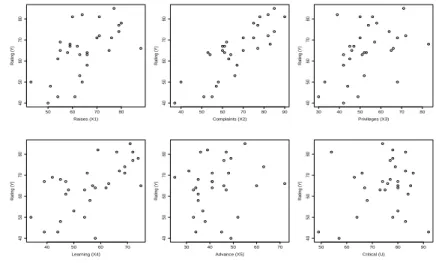
under-stand the effect of variables (X1, ..., X5 and U ) on Rating (Y ). Figure 2 plots
each independent variable against the response Y . We can see that the effect of U on Y is not linear, while the effect of other variables are roughly linear. So we employ the following model,
Y = a + β1X1+ β2X2+ β3X3+ β4X4+ β5X5+ f (U ) + ϵ. (12)
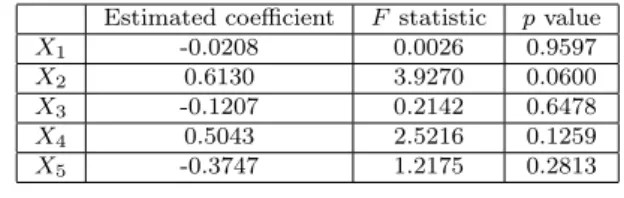
Using the estimation procedure discussed in Section 3 with m = 2, the linear
50 60 70 80 40 50 60 70 80 Raises (X1) Rating (Y) 40 50 60 70 80 90 40 50 60 70 80 Complaints (X2) Rating (Y) 30 40 50 60 70 80 40 50 60 70 80 Privileges (X3) Rating (Y) 40 50 60 70 40 50 60 70 80 Learning (X4) Rating (Y) 30 40 50 60 70 40 50 60 70 80 Advance (X5) Rating (Y) 50 60 70 80 90 40 50 60 70 80 Critical (U) Rating (Y)
Fig 2.Plot s of the individual explanatory variables against the response variable.
component in the model (12) is estimated as 18.1127− 0.0208X1+ 0.6130X2−
0.1207X3+ 0.5043X4− 0.3747X5. The F statistic and the p value for testing
each coefficient Hi0 : βi = 0 against Hi1 : βi ̸= 0 are given in Table 6. The
Estimated coefficient F statistic p value X1 -0.0208 0.0026 0.9597 X2 0.6130 3.9270 0.0600 X3 -0.1207 0.2142 0.6478 X4 0.5043 2.5216 0.1259 X5 -0.3747 1.2175 0.2813 Table 6
The estimated coefficients of the linear component and the significance tests.
We thus perform the simultaneous F test to test the hypothesis H0 : β1 =
β3 = β5 = 0 against H1 : at least one of them is nonzero. The value of the F
statistic is 2.1577 and the p value is 0.1206. In comparison, the value of the F
statistic for the global hypothesis H0 : β1 =· · · = β5 = 0 is 18.4038 and the p
value is less than 0.0001. The results show that we fail to reject the hypothesis
H0: β1= β3= β5= 0. We can thus refine the linear component by using only
Learning (X2) and Complaints (X4) as independent variables. In this case, the
estimated linear component is 16.3467 + 0.6725X2+ 0.2068X4. The F value for
this model is 34.3635 and p value is less than 0.0001.
50 60 70 80 90 −20 −10 0 10 20 Critical rating 50 60 70 80 90 −20 −10 0 10 20 Critical Nonpar ametr ic par t of r
ating from full model
50 60 70 80 90 −20 −10 0 10 20 Critical Nonpar ametr ic par t of r
ating from submodel
Fig 3.Kernel estimates of the nonparametric component f . The points are the residuals
of respective linear fits.
We can then estimate the nonparametric component of the effect of Critical (U ). For this, we run kernel estimation using the residuals of the linear fits as we did in Section 5.1. Figure 3 shows the nonparametric fits. The left panel plots the estimate of f under the model (12) but we ignore the linear component, the middle panel plots the estimate of f under the model (12) with all linear
variables and the right panel plots ˆf with the variables X2and X4in the linear
part. We can see that the plot on the left panel is quite different from the other two. And the two plots on middle and right are similar since including a small number of additional non-significant variables does not have a large effect on the
estimates of the remaining parts of the model. Moreover, we test the significance
of the nonparametric function, i.e. H0: f (u) = a + bu for some constants a, b. We
follow the test procedure described in [17]. The p-value of the likelihood ratio test is 0.043, which shows the nonparametric function is significant. Actually, we have significant result with p-value 0.0259 when we fit a quadratic function to the nonparametric component.
Note that in [8], the standard multiple linear regression was used to model the relationship between the response and the explanatory variables. The linear model failed to detect the relation of the variable U and Y , and it concluded that variable U did not have significant effect on Y .
6. Proofs
We shall prove Theorems 1, 3, 4, ,5 and 6. The proof of Theorem 7 is similar to that of Theorem 3 and Theorem 6, respectively. We will first prove some technical lemmas.
6.1. Technical Lemmas
Lemma 2 Under the assumptions of Theorem 1,
√
n(Z′Z)−1Z′w−→ N(0, (1 + O(mL −1))σ2Σ−1X ).
Proof. The asymptotic normality of √n(Z′Z)−1Z′w follows from the
Cen-tral Limit Theorem and the fact that ∑mk=1c2
k = O(m−1). It is known that
E(√n(Z′Z)−1Z′w) = 0 and V ar((Z′Z)−1Z′w|Z) = (Z′Z)−1Z′ΨZ(Z′Z)−1.
Note that with m = o(n), son1(Z′Z)−→ E[(a.s.
m+1∑ t=1 dtXi+m+1−t)( m+1∑ t=1 dtXi+m+1′ −t)] =
ΣX. Also with m = o(n), for any k = 1, 2,· · · , m,
1 n ∑n−m−1−k i=1 ( ∑m+1 t=1 dtXi+m+1−t)( ∑m+1 t=1 dtX ′ i+k+m+1−t) a.s. −→ ckΣX.
This implies nV ar((Z′Z)−1Z′w|Z) −→ σa.s. 2Σ−1X ΣX(1 + 2
m ∑ k=1 c2k)Σ−1X = (1 + O(1 m))σ 2Σ−1 X . So √ n(Z′Z)−1Z′w−→ N(0, (1 + O(L 1 m))σ 2Σ−1 X ).
Lemma 3 Under the assumptions of Theorem 1,
nE[((Z′Z)−1Z′δ)((Z′Z)−1Z′δ)′]= O( (m n )2(α∧1) ) (ΣX)−1 Proof.
Note that E(∑ni=1−m−1(∑m+1t=1 dtXi+m+1′ −t)δi) = 0, so E{(Z′Z)−1Z′δ} = 0.
Now E [ ( n−m−1∑ i=1 Ziδi)( n−m−1∑ i=1 Zi′δi) ] = ( n−m−1∑ i=1 δi2− ck n−m−2∑ j=1 δj m ∑ l=1 δj+m)ΣX.
When m = o(n), since f∈ Λα(M ),|δ i| < M(mn)(α∧1). So ∑n−m−1 i=1 δ 2 i − 1 m ∑n−m−2 j=1 δj ∑m l=1δj+m = O(n1−2(α∧1)m2(α∧1)).
Also we know that 1nZ′Z −→ Σa.s. X, therefore, as n→ ∞,
nV ar((Z′Z)−1Z′δ) = nO(n 1−2(α∧1)m2(α∧1)) n2 (ΣX) −1= O((m n )2(α∧1) ) (ΣX)−1.
The following lemma bounds the difference between the DWT of a sampled function and the true wavelet coefficients. See, for example, [3].
Lemma 4 Let ξJ,k=⟨f, ϕJ,k⟩ and n = 2J. Then for some constant C > 0,
sup V∈Λβ(M ) n ∑ k=1 (ξJ,k− n− 1 2V (k n)) 2≤ Cn−(2α∧1).
The following lemma is from [5].
Lemma 5 Let y = θ + Z, where θ is an unknown parameter and Z is a random
variable with EZ = 0. Then
E(η(y, λ)− θ)2≤ θ2∧ (4λ2) + 2E(Z2I(|Z| > λ)).
Lemma 6 Under the assumptions of Theorem 5, V ar(n1∑ni=1−1X(i)X(i+1)′ )→ 0
as n→ ∞. Here the variance and the limitation are both entry-wise.
Proof. First we have
V ar(1 n n−1 ∑ i=1 X(i)X(i+1)′ ) = 1 n2 n−1 ∑ i=1
V ar(X(i)X(i+1)′ ) +
2
n2
n∑−2
i=1
Cov(X(i)X(i+1)′ , X(i+1)X(i+2)′ )
+2
n2
∑
i+1<j
Cov(X(i)X(i+1)′ , X(j)X(j+1)′ ).
Here the covariance of two matrix means the covariance of corresponding entries.
Let ηi= h(U(i+1))−h(U(i)) and Hi= h′(U(i))h(U(i)) for i = 1, 2,· · · , n−1. Note
that when γ > 0, ηi= O(n−γ). Then for i+1 < j, Cov(X(i)X(i+1)′ , X(j)X(j+1)′ ) =
Cov(Hi, Hj) + O(n−γ). Hence,
2
n2
∑
i+1<j
Cov(X(i)X(i+1)′ , X(j)X(j+1)′ ) = V ar(
1 n n ∑ i=1 Hi) + O(n−γ).
Also, it is easy to see that 1
n2
∑n−1
i=1 V ar(X(i)X(i+1)′ ) = O(
1 n) and 2 n2 n∑−2 i=1
Cov(X(i)X(i+1)′ , X(i+1)X(i+2)′ ) = O(
1
n).
Putting these together, the lemma is proved.
Remark 12 By the same calculation, we actually can prove that for any fixed
integer k > 0, V ar(1n∑ni=1−kX(i)X(i+k)′ ) goes to zero as n goes to infinity.
6.2. Proof of Lemma 1.
It follows from Lemma 6 and the fact m = o(n) that lim n→∞V ar( Z′Z n ) = limn→∞V ar( Z′ΨZ n ) = limn→∞V ar( Z′δδ′Z n ) = 0.
So we only need to check the limit of the expectation. First note that
E(ZiZi′) =
m+1∑
t=1
d2tE(V ar(X(i+t−1)|U))+[
m+1∑ t=1 dth(U(i+t−1))]′[ m+1∑ t=1 dth(U(i+t−1))], E(ZiZi+j′ ) = m+1∑−j t=1
dt+jdtE(V ar(X(i+j+t−1)|U))+[
m+1∑ t=1 dth(U(i+t−1))]′[ m+1∑ t=1 dth(U(i+j+t−1))]. This implies lim n→∞E( Z′Z n ) = limn→∞ 1 n n−m−1∑ i=1 E(ZiZi′) = limn→∞ 1 n n ∑ i=1
E[V ar(Xi|U)] = Σ∗.
Here we use the fact that, since h(U ) has γ > 0 derivatives. Similarly, limn→∞n1E(Z′ΨZ) =
(1− Σc2
k)Σ∗. Finally for the third equation, let dhi =
∑m+1 t=1 dth(U(i+t)) 1 nE(Z ′δδ′Z) = 1 n n ∑ i=1
E[V ar(X(i)′ |U)(∑
t d2tδi2−t+ m+1∑ t=1 m+1∑ k=1 dtdt+kδi−tδi+k−t)] +1 n[ n ∑ i=1 δiE(dhi)]′[ n ∑ i=1 δiE(dhi)] Since ∑td2tδ2i−t+ ∑m+1 t=1 ∑m+1
k=1 dtdt+kδi−tδi+k−t is of order n−2α for any i,
the first part of the above expression is of order n−2α. And δiE(dhi) is of order
n−α−γfor any i, so the second part of the above expression is of order n1−2α−2γ.
This implies 1
nE(Z
′δδ′Z) = O(n−2α) + O(n1−2α−2γ
6.3. Proofs of Theorems
Theorem 1 now follows from Lemmas 2 and 3. Note that√n( bβ−β) =√n(Z′Z)−1Z′(w+
δ). Lemma 3 implies√n(Z′Z)−1Z′δ−→ 0. This together with Lemma 2 yieldP
Theorem 1.
For Theorem 3 ,we shall only prove the convergence rate under the pointwise squared error loss, the rate of convergence under the global mean integrated squared error risk can be derived using a similar line of argument.
Let ˆf1(u) = ∑ni=1Ki,h(u)(f (Ui) + ϵi) and ˆf2(u) =
∑n
i=1Ki,h(u)Xi(β −
ˆ
β) + ˆa− a, then ˆf (u) = ˆf1(u) + ˆf2(u). In ˆf1 there is no linear component.
From the standard nonparametric regression results we know that for any x0,
supf∈Λα(M )E
[
( ˆf1(x0)− f(x0))2] ≤ Cn−2α/(1+2α) for some constant C > 0.
Note that∑ni=1K2
i,h(u) = O( 1 nh) = O(n−2α/(1+2α)). So E( ˆf2(x0)2) = E [ ( n ∑ i=1 Ki,hXi(β− ˆβ))2 ] ≤ n ∑ i=1
Ki,h2 E(Xi(β− ˆβ))2= O(n−2α/(1+2α))
Hence the Theorem is proved.
For Theorem 4, note that the maximum approximation error is of order n−(2α∧1) and is negligible relative to the minimax risk in Theorem 4. Now we shall only prove the upper bound for the integrated squared error. The case of local pointwise error is similar. Note that
E [∫ ( bf (x)− f(x))2dx ] = E∑ k ( ˆξj0,k−ξj0,k) 2+E J1 ∑ j=j0 ∑ k (ˆθj,k−θj,k)2+ ∑ j>J1 ∑ k θ2j,k. (13)
Note that for θj,k=⟨f, ψj,k⟩, there exists a constant C > 0 such that for all
j≥ j0, 1≤ k ≤ 2j
sup
f∈Λα(M )|θ
j,k| ≤ C2−j(α+1/2). (14)
See [12]. Hence supf∈Λα(M )
∑ j>J1 ∑ kθ 2 j,k≤ C2−J12α= o(n−2α/(1+α)).
This means the third term in equation (13) is negligible. So we just need
to focus on the first two terms. We know that E( ˆξj0,k− ξj0,k)
2 ≤ 2E(˜τ2 j0,k) + 2 nE(˜z 2 j0,k) and E(ˆθj,k− θj,k) 2 ≤ 2E(τ2 j,k) + 2E(ηλ(θj,k + n−1/2zj,k)− θj,k)2.
Putting them together, we have E[ ∫ ( bf (x)− f(x))2dx] = 2E∑ j,k (ηλ(θj,k+ n−1/2zj,k)− θj,k)2+ 2 nE ∑ k (˜z2j0,k) +2E(∥X( ˆβ − β) + (ˆa − a) · 1n∥22).
where 1n denotes the n dimensional column vector of 1. From Theorem 1 and
Theorem 5, we know that E(∥X( ˆβ − β)∥2
2) =n1E(XΣ−1X′) = O(
1
n) and E(ˆa−
a)2 = O(n−1∧ n−2α). This means the third term is negligible relative to the
minimax rate. Also we know that there are only a fixed number of terms in the sum of the second term, so this term is also negligible. From now on, we just need to focus on the first term.
From lemma 5, E∑j,k(ηλ(θj,k + n−1/2zj,k)− θj,k)2 ≤ ∑ θ2 j,k ∧ (4λ2) + ∑2 nE(z 2
j,kI(|zj,k| ≥ n1/2λ)) , S1+ S2. By the same argument as the proof
of Theorem 1 in [5], we can show that S2is negligible as compared to results of
the Theorem 4.
For S1, it can be seen that when j ≥
J−log2J 2α+1 , equation (14) yields θ 2 j,k∧ (4λ2) ≤ θ2 j,k ≤ C2−j(1+2α) and when j ≤ J−log2J 2α+1 , θ 2 j,k ∧ (4λ2) ≤ 4λ2 ≤
Clog nn for some constant C > 0. This means S1 ≤ ∑j≤J−log2 J
2α+1 C2j(log n n ) + ∑ j>J−log2 J2α+1 C2−2jα≤ C( log n n )
2α/(1+2α). Hence the Theorem is proved.
Now we will prove Theorem 5. With Lemmas 1 and 2, the proof of
The-orem 5 is now straightforward. Note that √n( ˆβ − β) = √n(Z′Z)−1Z′w +
√
n(Z′Z)−1Z′δ. It follows from the same argument as in the proof of Lemma 2
that √n(Z′Z)−1Z′w ∼ N(0, n(Z′Z)−1Z′ΦZ(Z′Z)−1). The first two equalities
of Lemma 1 yields lim
n→∞n(Z
′Z)−1Z′ΦZ(Z′Z)−1) ={Σ ∗}−1
and the third equality of Lemma 1 shows that, when α+γ > 1/2,√n(Z′Z)−1Z′δ
is small and negligible. Theorem 5 now follows.
Next we will prove Theorem 6. Let L be a (n− m) × n matrix given by
Li,j=
{
dj−i+1 for 0≤ j − i ≤ m
0 otherwise . (15)
Moreover, let J be another (n− m) × n matrix given by Ji,i = 1 for i =
1, 2,· · · , n − m and 0 otherwise. Then w = Lϵ = Jϵ + (L − J)ϵ = w1+ w2
where w1 = J ϵ and w2 = (L− J)ϵ. We can see that w1 ∼ N(0, σ2In−m) and
w2∼ N(0, σ2(L− J)(L − J)′). Note that d21= 1− O(m−1), hence each entry of
the covariance matrix of w2 is of order m−1. So w2 goes to 0 in probability as
n goes to infinity and is negligible as compared to w1.
We know that ˆβ = β+(Z′Z)−1Z′w = β+(Z′Z)−1Z′w1+(Z′Z)−1Z′w2. Hence
under H0, C ˆβ = C(Z′Z)−1Z′w1+ C(Z′Z)−1Z′w2, where C(Z′Z)−1Z′w1 ∼
N (0, σ2C(Z′Z)−1C′).
On the other hand, w′Hw = w1′Hw1+ 2w1′Hw2+ w′2Hw2. It is easy to check
that H is a projection of rank n−m−p, i.e., H2= H and rank(H) = n−m−p.
Hence w1′Hw1= (Hw1)′(Hw1) follows a χ2distribution with n−m−p degrees of
freedom. Now we know that σ12w1′Z(Z′Z)−1C′(C(Z′Z)−1C′)−1C(Z′Z)−1Z′w1
follows χ2(r) and w′1Hw1follows χ2(n− m − p) and they are independent. This
By the same argument as in the proof of Theorem 1, we can prove that the asymptotic power of this test (at local alternatives) is the same as the usual F test when f is not present in the model (1).
References
[1] Bickel, P. J., Klassen, C. A. J., Ritov, Y. and Wellner, J. A. (1993). Efficient and Adaptive Estimation for Semiparametric Models. The John Hopkins University Press, Baltimore.
[2] Brown, L.D. and Low M.G. (1996). A Constrained Risk Inequality with Applications to Nonparametric Functional Estimations. Ann. Statist. 24, 2524-2535.
[3] Cai, T. and Brown, L.D. (1998). Wavelet shrinkage for nonequispaced sam-ples. Ann. Statist. 26, 1783-1799.
[4] Cai, T., Levine, M., and Wang, L. (2009). Variance function estimation in multivariate nonparametric regression. Journal of Multivariate Analysis,
100, 126-136.
[5] Cai, T. and Wang, L. (2008). Adaptive variance function estimation in heteroscedastic nonparametric regression. Ann. Statist. 36, 2025C2054. [6] Carroll, R. J., Fan, J., Gijbels,I., and Wand, M. P. (1997). Generalized
partially linear single-index models. J. Amer. Statist. Assoc. 92, 477-489. [7] Chang, X., and Qu, L. (2004). Wavelet estimation of partially linear models.
Comput. Statist. Data Anal. 47, 31-48.
[8] Chatterjee, S. and Price, B. (1977). Regression Analysis by Example. New York: Wiley.
[9] Chen, H. and Shiau, J. H. (1991). A two-stage spline smoothing method for partially linear models. J. Statist. Plann. Inference 27, 187-201. [10] Cuzick, J. (1992). Semiparametric additive regression. J. Roy. Statist. Soc.
Ser. B 54, 831-843.
[11] Dawber, T. R., Meadors G. F., and Moore F. E. J. (1951). Epidemiological approaches to heart disease: the Framingham Study. Amer. J. Public Health
41, 279-86.
[12] Daubechies, I. (1992). Ten Lectures on Wavelets. SIAM, Philadelphia. [13] Donoho, D.L. and Johnstone, I.M. (1994). Ideal spatial adaptation via
wavelet shrinkage. Biometrika 81, 425-55.
[14] Engle, R. F., Granger, C. W. J., Rice, J. and Weiss, A. (1986). Nonpara-metric estimates of the relation between weather and electricity sales. J. Amer. Statist. Assoc. 81, 310-320.
[15] Fan, J., and Huang, L. (2001). Goodness-of-Fit Tests for Parametric Re-gression Models. J. Amer. Statist. Assoc. 96, 640-652.
[16] Fan, J., and Zhang, J. (2004). Sieve empirical likelihood ratio tests for nonparametric functions. Ann. Statist. 32, 1858-1907.
[17] Fan, J., Zhang, C. and Zhang, J. (2001). Generalized likelihood ratio statis-tics and Wilks phenomenon. Ann. Statist. 29, 153-193.
[18] Gannaz, I. (2007). Robust estimation and wavelet thresholding in partially linear models. Statist. Comput. 17, 293-310.
[19] Hall, P., Kay, J. and Titterington, D. M. (1990). Asymptotically opti-mal difference-based estimation of variance in nonparametric regression. Biometrika 77, 521-528.
[20] Hamilton, S., and Truong, Y. (1997). Local linear estimation in partly linear models. J. Multivariate Anal. 60, 1C19.
[21] H¨ardle, W. (1991). Smoothing Techniques. Berlin: Springer-Verlag.
[22] Horowitz, J. and Spokoiny, V. (2001). An adaptive rate-optimal test of a parametric mean-regression model against a nonparametric alternative. Econometrica 69, 599-631.
[23] Lam, C., and Fan, J. (2007). Profile-Kernel Likelihood Inference With Di-verging Number of Parameters. Ann. Statist. , to appear.
[24] Liang, H., H¨ardle, W. and Carroll, R. J. (1999). Estimation in a
semipara-metric partially linear errors-in-variables model. Ann. Statist. 27, 1519-1535.
[25] M¨uller, M. (2001). Estimation and testing in generalized partial linear
mod-elsA comparative study. J. Statist. Comput. 11, 299-309.
[26] Munk, A., Bissantz, N., Wagner, T. and Freitag, G. (2005). On difference based variance estimation in nonparametric regression when the covariate is high dimensional. J. Roy. Statist. Soc. B 67, 19-41.
[27] Rice, J. A. (1984). Bandwidth choice for nonparametric regression. Ann. Statist. 12, 1215-1230.
[28] Ritov, Y., and Bickel, P. J. (1990). Achieving information bounds in semi and non parametric models. Ann. Statist. 18, 925-938.
[29] Robinson, P. M. (1988). Root-N consistent semiparametric regression. Econometrica. 56, 931-954.
[30] Scott, D. W. (1992). Multivariate Density Estimation. New York: Wiley. [31] Severini, T. A. and Wong, W. H. (1992). Generalized profile likelihood and
conditional parametric models. Ann. Statist. 20, 1768-1802.
[32] Speckman, P. (1988). Kernel smoothing in partial linear models. Jour. Roy. Statist. Soc.Ser. B 50, 413-436.
[33] Schimek, M. (2000). Estimation and inference in partially linear models with smoothing splines. J. Statist. Plann. Inference 91, 525C540.
[34] Strang, G. (1989). Wavelet and dilation equations: A brief introduction. SIAM Rev. 31, 614-627.
[35] Tjøstheim, D., and Auestad, B. (1994). Nonparametric Identification of Nonlinear Time Series: Projection. J. Amer. Statist. Assoc. 89, 1398-1409. [36] Wahba, G. (1984). Cross validated spline methods for the estimation of multivariate functions from data on functionals. Statistics: An Appraisal. Proceedings 50th Anniversary Conference Iowa State Statistical Laboratory (H. A. David, ed.). Iowa State Univ. Press.
[37] Wang, L., Brown, L.D., Cai, T. and Levine, M. (2008). Effect of mean on variance function estimation on nonparametric regression. Ann. Statist. 36, 646C664.
[38] Yatchew, A. (1997). An elementary estimator of the partial linear model. Economics Letters 57, 135-143.