Discovering network topology by correlating end-to-end delay measurements

(1)

Discovering Network Topology by Correlating

End-to-end Delay Measurements

by

Jason Ivan Howard Baron

B. S., Computer Science and Engineering Massachusetts Institute of Technology (2000)

Submitted to the Department of Electrical Engineering and Computer Science in Partial Fulfillment of the Requirements for the Degree of

Master of Engineering in Electrical Engineering and Computer Science at the

Massachusetts Institute of Technology

February 6, 2001

The author hereby grants to M.I.T. permission to reproduce and distribute publicly paper and electronic copies of this thesis and to grant others the right to do so.

Author……… Department of Electrical Engineering and Computer Science

Februrary 6, 2001 Certified by………

Mark W. Garrett VI-A Company Thesis Supervisor Telcordia Technologies Certified by………

Hari Balakrishnan Assistant Professor M.I.T. Thesis Supervisor Accepted by………

Arthur C. Smith Chairman, Department Committee on Graduate Theses

(2)

(3)

Discovering Network Topology by Correlating

End-to-end Delay Measurements

by

Jason Ivan Howard Baron

Submitted to the Department of Electrical Engineering and Computer Science February 6, 2001

In Partial Fulfillment of the Requirements for the Degree of Master of Engineering in Electrical Engineering and Computer Science

Abstract

Conventional methods of discovering network topology require the cooperation of network elements. We present a method of network topology discovery based solely upon end-to-end delay measurements that requires only the cooperation of end systems. Previous work using end-to-end measurements has focused on discovering tree

topologies; the method here discovers more general networks. The discovery method is based on two algorithms: the matroid algorithm and the correlation algorithm. This work develops and validates the correlation algorithm for three increasingly sophisticated network models using simulation. We also develop an indicator of the quality of a particular result.

VI-A Company Thesis Supervisor: Mark W. Garrett

Title: Director, Internet Performance Research Group, Telcordia Technologies, Inc. Thesis Supervisor: Hari Balakrishnan

(4)

(5)

Acknowledgements

Writing an acknowledgement section is difficult for three reasons. First, a thesis is only possible because of the efforts of many individuals. Therefore, it is incumbent upon the author to not forget anyone worthy of credit. Second, the acknowledgement section is the only section of the thesis where the author can freely express personality. Thus, the author must be sure to be witty and funny, or at least make some semblance of wit and humor, because there are no other opportunities to do so. Finally, an acknowledgement section is written last, immediately after the thesis supervisor has approved the work*. Therefore, the author must make haste before the supervisor has a change of heart. With an understanding of the difficulties of the

acknowledgement section in hand and a little more serious tone, we proceed.

Dr. Mark Garrett was the most involved, enthusiastic, and insightful supervisor that one could have. Over two years ago, when I was deciding what to focus my masters research on, Mark presented the Felix project to me in such a way that I knew that I had to work for him. Mark’s sense of humor helped keep the research fun. For instance, my progress was sometimes

measured by Mark holding up the stack of papers that constituted my current version of the thesis and exclaiming: “Feels heavier than before, good!”.

When I introduced my thesis topic to Professor Hari Balakrishnan, he joked that I should work with him at MIT, instead of for Mark at Telcordia. Despite the distance between Telcordia and MIT, I often felt like Hari was in the next room because he would reply immediately to my e-mails.

Many ideas came out of conversations with the mathematician, Dr. David Shallcross. David’s keen interest in my work was very refreshing. Special thanks to Professor Paul Seymour for developing the matroid algorithm that paved the way for this work. Many thanks to Dr. Brian Coan, who having gotten his doctorate at MIT, gave me perspective and insight into the thesis process. Thank you Dr. Will Leland for ensuring that my thesis did not reveal too many of Telcordia’s secrets.

Fellow 6A’er, officemate, and lunchmate Gina Yip was an amazing friend. We had great conversations about all of the major events that transpired during the summer and fall semesters, including the Olympics, the subway series, and the improbable presidential election, that we showed was not so improbable after all**.

Finally, I must thank all of my friends who through the following biweekly exchange made me finish my thesis in a timely fashion. Friend: “So, you finished yet?” Me: “Perhaps, another two weeks, it looks like now.” Friend: “That’s what you said two weeks ago.” Me: “Yea, and I’m probably going to say it again in another two weeks.”

I guess I must now thank family, since family get-togethers are tough enough as it is. I thank my cousins Brant and Joel, and my Aunt Sarah for providing constant laughter and love.

I am forever grateful to my parents for their love and support. They have taught me the value of hard work as Vince Lombardi aptly once said: “The dictionary is the only place that ‘success’ comes before ‘work’.”

Finally, I would like to thank Dr. Kenneth Calvert, Dr. Matthew Doar, and Dr. Ellen Zegura for the freely available tiers software that was used in our simulations.

*_{Although we do not have sufficient empirical evidence to support this claim, we nevertheless believe it to} be the case.

(6)

(7)

List of Figures

Figure 1-1: The topology discovery method... 12

Figure 2-1: Illustration of network terminology. ... 17

Figure 2-2: Example of a path’s end-to-end delay time series. ... 18

Figure 2-3: Series links.. ... 20

Figure 2-4: Consecutive equivalent links.. ... 21

Figure 2-5: Eliminating consecutive equivalent links ... 22

Figure 2-6: Non-consecutive equivalent links.. ... 23

Figure 2-7: Original network topology generated by tiers... 24

Figure 2-8: Visible network.. ... 24

Figure 2-9: Reduced network... 24

Figure 2-10: Code tool-chain………...…….25

Figure 3-1: Applying a threshold. ... 29

Figure 3-2: Binary functions. ... 30

Figure 3-3: Circling algorithm.. ... 31

Figure 3-4: 2-path trigger probabilities... 33

Figure 3-5: Pseudocode of the correlation algorithm. ... 36

Figure 3-7: Discovered network.. ... 40

Figure 4-1: Calculating an observation probability. ... 44

Figure 4-2: Relating trigger probabilities to observation probabilites... 47

Figure 4-3: Pseudocode of the calculate-trigger-probability procedure. ... 58

Figure 4-4: Psuedocode of the correlation algorithm. ... 59

Figure 4-5: Sample network topology for demonstrating the correlation algorithm ... 60

Figure 4-6: Path-link matrix for the network shown in Figure 4-5... 60

Figure 4-7: Binary tree constructed by the correlation algorithm... 61

Figure 4-8: Distribution of the true and false leads.. ... 62

Figure 4-9: Simulation length as a function of the number links. ... 67

Figure 4-10: Running time of the correlation algorithm... 68

Figure 4-11: Varying the link congestion rates... 69

Figure 4-12: Reduced network used for varying the link congestion rates.. ... 70

Figure 4-13: Reduced network………..71

Figure 5-1: Sample of several paths’ binary functions. ... 76

Figure 5-2: Setting of the pruning_threshold and the final_pruning_threshold... 77

Figure 5-3: Running time of the correlation algorithm... 78

Figure 5-4: Histogram of separated fully specified trigger probabilities... 79

(10)

(11)

Chapter 1 Introduction

1.1 Motivation

Knowledge of network topology is essential for network management and network provisioning. However, conventional methods of network discovery (e.g., SNMP-based autodiscovery) rely on the cooperation of network elements and therefore have several potential shortcomings. For instance, network elements may be uncooperative due to heavy loading that disables autodiscovery in order to reduce processor load. Or, the owner of the network elements might restrict their access rights.

In addition, network elements may not have the functionality that is desired.

Traditional autodiscovery tools may use outdated protocols or protocols that have not yet been implemented by network elements. Autodiscovery tools may also be limited because they can only detect the logical connectivity of a particular network layer. For example, ICMP and traceroute can not detect ATM switches.

A discoverer may not want network elements to be aware of the discovery process. In a military context, we might want to make a map of the enemy’s network. Or, an ISP might want to verify the connectivity of a carrier network in order to verify service agreements.

This work responds to these concerns and provides a starting point for a system that can discover a broad class of network topologies from end-to-end delay measurements. The work grows out of a 1997 DARPA proposal by Christian Huitema at Telcordia Technologies. The proposal received funding and became the Felix Project [6, 7]. The

(12)

Felix Project focused on using non-invasive end-to-end measurements to determine network characteristics.

End-to-end measurements only require that the end systems be centrally controlled. Any interior network elements may be uncooperative to the extent that they do not respond to direct probing, such as ICMP, but they do forward probe packets. The topology discovery method presented here is based on two algorithms: the correlation algorithm and the matroid algorithm.

1.2 Correlation and Matroid Algorithms

Monitors collect the end-to-end delay measurements that are the starting point for discovering network topology. Monitors are placed at certain nodes in the network and collect delay measurements by time-stamping packets that are sent to other monitors. The links in a network that are traversed when a monitor sends a packet to another monitor constitute a path. The collected data is organized as end-to-end delay time as a function of time for each path.

The collected data is then used to discover the topology of the network in two steps. First, the correlation algorithm determines the links in the network by correlating the times when paths exhibit common end-to-end delay characteristics. The output of the correlation algorithm is a path-link matrix that identifies which links are on which paths. The matroid algorithm (invented by P. D. Seymour) [7] then reconstructs the network topology based upon the path-link matrix. The solution method is illustrated in Figure 1-1.

Figure 1-1: The topology discovery method.

end-to-end delay measurements path-link matrix discovered network topology correlation matroid

(13)

The matroid algorithm uses linear algebra and graph theory to construct the network topology from the path-link matrix. The path-link matrix does not necessarily completely determine the network topology. For example, the matroid algorithm may produce a network that contains split nodes, which are a set of nodes in the discovered network that correspond to the same node in the original network. The matroid algorithm can also output localized uncertainties in the network topology or clouds. For the purposes of this paper, the matroid algorithm is treated as a black box.

The contribution of this thesis is the development and validation of topology

discovery algorithms based upon the idea of correlating common end-to-end delay time characteristics that occur on network paths. Three correlation algorithms that are based upon accompanying network models form the core of the work. We start with relatively simplistic network models and move towards more complex ones. Validation of the correlation algorithms is done using simulation. We use simulation instead of real-world traffic data because exploring the ideas of the correlation algorithm would initially be too difficult with real-world data.

1.3 Related Work

A number of related papers have been published recently. We classify this related work into three areas: end-to-end measurement systems, analysis and modeling of real-world end-to-end measurements, and analysis and modeling of simulated end-to-end measurements. The present work belongs in the third area, analysis and modeling of simulated end-to-end measurements.

Measurement systems are primarily concerned with how end-to-end measurements can be made accurately and what type of infrastructure is required to support these measurements. These projects are concerned with many systems related issues such as scaling, distributed computing, and security. The National Internet Measurement Infrastructure (NIMI) project [13] proposes to build a large-scale measurement

infrastructure on top of the existing Internet, similar to the Domain Name System. NIMI is primarily concerned with scalability and security. Another significant measurement

(14)

system is Surveyor [20], consisting of 38 machines spread around the world. One-way delay and packet loss is measured between these machines. Additional projects in this area are: Skitter [19], Internet Performance Measurement and Analysis (IPMA) at Merit [11], and Internet Monitoring & PingER at Stanford Linear Accelerator Center (SLAC) [10].

The second area of related work is analysis and modeling of real world end-to-end measurements. This work uses end-to-end measurements from real-world network traces to infer characteristics about the network. Most of the work focuses on analyzing delay and loss models. For example, Yajnik et al. [23] present a method of estimating the loss rates on links of a known multicast tree topology using the receivers’ loss patterns. Further references in this area include [1, 12, 14, 24].

The third broad area of related work that we consider is analysis and modeling of simulated end-to-end measurements. A number of simulation studies have been done on inferring characteristics of multicast tree networks based upon the loss patterns of

receivers. Caceres et al. [3] and Ratnasamy et al. [17] have developed maximum

likelihood estimations of multicast tree topologies and the packet loss rates on these links. The basic insight is that if a multicast packet is lost along a link in the tree, all intended recipients lower in the tree will be affected. Intuitively, the closer the loss pattern of two receivers, the more likely it is that they are closely related in the multicast tree.

Moving from multicast to unicast streams but still considering only tree topologies, Rubenstein et al. [18] and Harfoush et al. [9] suggest two different probing packet techniques for characterizing the internals of a network. Rubenstein et al. propose analyzing two Poisson probe flows in order to detect if two co-located receivers or two co-located senders have shared points of congestion. Harfoush et al. suggest a method of identifying shared loss by using Baysian probes. Harfoush et al. are able to reconstruct the tree topology and loss rates between a server and a set of clients using these probes. Further references in this area include [2, 5, 16].

(15)

In the present work, we address the problem of inferring network topology for a mesh of paths. We are not limited to tree topologies in any way. In addition to discovering the network topology, we provide an estimate of individual link congestion rates.

1.4 Outline

We present background material and the network topology generation process in Chapter 2. Chapters 3, 4, and 5 delve into the three network models that form the core of the work. Each of these chapters contains an explanation of the network model, a correlation algorithm, results, and discussion. Finally, we present conclusions and future work in chapter 6.

(16)

Chapter 2 Background

Before we examine the three network models that form the core of this paper in chapters 3, 4 and 5, we present background material. In section 2.1, we introduce

terminology that will be used extensively throughout the paper. Section 2.2 explains how we generate the network topologies that are used for testing the topology discovery algorithms. Finally, in section 2.3, we present an overview of how the various pieces of code fit together.

2.1 Terminology

We define a network as a set of nodes and directed edges, or links. Special nodes in the network are monitors. Nodes that are not monitors are interior nodes. A path is the set of nodes and links that are traversed if data is sent from one monitor to another monitor. Paths are simple, having no repeated nodes or links and consequently do not have loops. Paths are not necessarily symmetric. That is, the set of nodes that is

traversed on the path between monitor M1 and monitor M2 need not be the same as the set of nodes that is traversed by the path from monitor M2 to M1. A path that is not

symmetric is asymmetric. Paths are also stable. A stable path is a path does not change over time. Figure 2-1 illustrates these concepts.

(17)

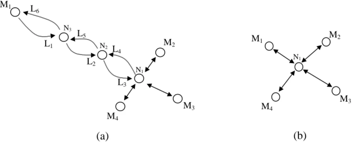
Figure 2-1: Illustration of network terminology.

The network in Figure 2-1 has eleven nodes. Five of these nodes are monitors and they are labeled: M1, M2, M3… The six interior nodes are labeled: N1, N2, N3… Some links are labeled next to arrowheads that indicate the direction of the link. The links that constitute path p are: L1, L2, L3, L4, and L5, while the links that constitute path q are: L2, L6, L7, and L8.

All of the network models are based upon packet-switched networks. By time-stamping the packets that are sent from one monitor to another, the end-to-end delay time for a path is recorded. If time-stamped packets are sent over time, then the end-to-end delay time series from one monitor to another or a path’s end-to-end delay time series is constructed. Figure 2-2 is an example of such a time series.

path p path q L2 L3 L4 L5 L7 L8 M1 M5 M2 M3 M4 L1 L6 N1 N3 N2 N4 N5 N6

(18)

Figure 2-2: Example of a path’s end-to-end delay time series. Note that this time series is only illustrative and is not meant to represent a recorded time series. In practice, the time series tends to

be more punctuated and not as smooth as what is illustrated.

Finally, we formalize the path-link matrix that was introduced in chapter 1. One axis of the matrix is indexed by a path name and the other axis is indexed by a link name. We put a 1 in position (i, j), if link j is on path i and a 0 otherwise. Constructing such a matrix for paths p and q, which are defined in Figure 2-1 yields:

L1 L2 L3 L4 L5 L6 L7 L8 L9

P 1 1 1 1 1 0 0 0 0

Q 0 1 0 0 0 1 1 1 0

The path-link matrix serves as the interface between the correlation algorithm and the matroid algorithm. Note that the path-link matrix does not indicate how many nodes are in the network, nor whether or not two different paths share common nodes. Unlike an adjacency-matrix representation of a graph, the path-link matrix does not necessarily completely specify a network’s topology.

2.2 Network Topology Generation and Reduction

In this section, we discuss the methodology we use to create network topologies for testing the topology discovery algorithms. We wanted a method that could generate a wide range of realistic network topologies, while keeping in mind the limitations of the discovery algorithms. Therefore, we create an initial randomized, realistic network topology using the tiers program by Calvert et al. [4]. Next, we choose a fixed number of

time d el ay tim e

(19)

leaf nodes at random as monitors. We remove nodes and links that are not traversed by any paths, creating the visible network. Finally, we simplify or reduce the visible network, creating the reduced network.

The tiers program generates randomized and realistic topologies according to a three tier hierarchical structure. The three tiers are: Wide Area Networks (WANs),

Metropolitan Area Networks (MANs), and Local Area Networks (LANs). Several parameters control graph generation. The user can specify the number of nodes in each type of network as well as the number of MANs per WAN, and LANs per MAN.

Additionally, the connectivity within a network and between different types of networks can be specified. We refer to the network generated by tiers as the original network. Monitors are then selected randomly from among the leaf nodes of the original

network. We choose the leaf nodes as monitors because they tend to be at the edge of the network and therefore much of the network is contained on the paths between them. If we chose monitors in the center of the network, then the network topologies would probably not be very complex or interesting.

Given the choice of monitors, we determine the paths based upon shortest hop routing. This is implemented using breadth first search from each monitor. This implementation lends itself to the generation of asymmetric paths. Empirical work by Vern Paxson [15] found that in one network approximately 30% of the paths exhibited asymmetry. We find paths generated using breadth first search to be asymmetric approximately 35% of time. We assume that the routing is stable and thus paths do not change over time. After removing the nodes and links that are not traversed by any paths in the original network, the visible network remains.

From the visible network, we proceed to reduce the graph. The correlation algorithm requires that each link in the network be traversed by a unique set of paths. The matroid algorithm assumes that all paths are simple, a monitor is not an interior node in the network, and that paths destined to the same monitor do not converge and then diverge. This final assumption of the matroid algorithm means that all paths into a monitor form a

(20)

The visible network satisfies the requirements of the matroid algorithm. A sink tree into each monitor is assured by using breadth first search because the adjacency list that is used to represent the network is examined in the same order in determining all paths. We ensure that monitors are not in the interior of the network by choosing monitors from among the leaf nodes in the original network. Finally, shortest hop paths do not contain any repeated nodes or links and therefore the simple path constraint is satisfied.

The visible network does not necessarily satisfy the correlation algorithm’s

requirement that each link be traversed by a unique set of paths. We classify links that are traversed by the same set of paths as other links into two categories: series links and

equivalent links. Series links can be found by identifying those nodes that have an

in-degree and out-in-degree of one or an in-in-degree and out-in-degree of two. To illustrate this concept, consider Figure 2-3.

Figure 2-3: Series links. Figure 2-3(a) contains 6 series links. Links L1, L2, and L3 are all traversed by paths M1-M2, M1-M3, and M1-M4, while links L4, L5, and L6 are traversed by paths M2-M1, M3-M1,

and M4-M1. Figure 2-3(b) modifies the network, eliminating the series links.

In Figure 2-3(a), nodes 2 and 3 both have an in-degree and out-degree of two. If we designate the path from M1 to M3 as M1-M3, then links L1, L2, and L3 are traversed by paths M1-M2, M1-M3, and M1-M4, while links L4, L5, and L6 are traversed by paths M2 -M1, M3-M1, and M4-M1. We can remove these series links by removing nodes 2 and 3 and reconnecting the graph as shown in Figure 2-3(b).

M4 M3 M1 M2 N3 N2 N1 L1 L2 L3 L4 L5 L6 M3 M4 M1 M2 N1 (a) (b)

(21)

An equivalent link is a link that is traversed by the same set of paths as at least one other link in the network, but it is not a series link. Equivalent links are further classified as consecutive equivalent links and non-consecutive equivalent links. A consecutive equivalent link has at least one node in common with another link that is traversed by the same set of paths as itself. A non-consecutive equivalent link is an equivalent link that does not have a common node with a link that is traversed by the same set of paths as itself.

In Figure 2-4, we present an example of consecutive equivalent links. The table in Figure 2-4(b) is an ordered set of the links that are traversed on each path. Notice that links L7 and L8 always appear together in the table and are found on paths M1-M2 and M3-M2. Looking at the network diagram, links L7 and L8 share a common node and are not series links. Therefore, links L7 and L8 are consecutive equivalent links. Links L2 and L10 are also consecutive equivalent links, while links L4 and L5 are series links.

Figure 2-4: Consecutive equivalent links. Links L7 and L8 share a common node and are traversed by paths M1-M2 and M3-M2. Thus, L7 and L8 are consecutive equivalent links. Links L2 and L10 are also consecutive equivalent links. The table in Figure 2-4(b) indicates the links that are traversed on the paths between the indicated monitors.

We modify the network that contains consecutive equivalent links as follows. We define a group of consecutive equivalent links as set of consecutive equivalent links where each link in the set is traversed by the same set of paths. We can move from the

M1-M2: L2, L10, L8, L7 M1-M3: L2, L10, L12 M2-M1: L6, L5, L4, L1 M2-M3: L6, L9, L12 M3-M1: L11, L3, L1 M3-M2: L11, L8, L7 L1 L2 L4 L3 L12 L7 L8 L5 L10 L9 L11 L6 M1 M2 M3 (a) (b)

(22)

begin node to the end node of a group of consecutive equivalent links by traversing only

and all of those links that are in the group. We remove all of the consecutive equivalent links in a group from the network and then add to the network a single link from the begin node to the end node. After modifying the network in this manner, we remove nodes that are no longer traversed by any path. Applying this procedure to Figure 2-4 results in network found in Figure 2-5.

Figure 2-5: Eliminating consecutive equivalent links. Consecutive equivalent links L2, L7, L8, and L10 are removed from the network in Figure 2-4(a). Links L13 and L14 are added to the network. In addition, the series links L4 and L5 are removed from Figure 2-4(a) and L15 is added.

An example of non-consecutive equivalent links is shown in Figure 2-6. In the figure, paths only traverse links that lie on the hexagon shape and links that are incident to a monitor, except for paths M1-M4, M4-M1, M3-M6, and M6-M3. These paths traverse links in the interior of the hexagon shape as shown. Links L2 and L4 are non-consecutive equivalent links, being traversed only by path M6-M3, while L1 and L3 are also non-consecutive equivalent links, being traverse only by path M3-M6. Paths M1-M4 and M4-M1 contain analogous non-consecutive equivalent links as well.

L1 L3 L12 L9 L11 L6 M1 M2 M3 L13 L15 L14

(23)

Figure 2-6: Non-consecutive equivalent links. Links L2 and L4 are only traversed by the path M6-M3 and are thus non-consecutive equivalent links. Similarly, links L1 and L3 are only traversed only by

the path M3-M6 and are thus non-consecutive equivalent links as well. Analogous non-consecutive links occur on the path M1-M4 and M4-M1.

A network that has been checked for series and consecutive equivalent links and modified appropriately is a reduced network. The reduced network may seem very different from the visible network. However, a network that is modified because of series links does not change the graph in any structurally significant ways. Modifications to network topology that are due to consecutive equivalent links are localized in the network and the number of links in a group of consecutive equivalent links is typically small*. Finally, we do not use networks that contain non-consecutive equivalent links. However, networks with non-consecutive equivalent links are extremely rare in practice**.

We show the evolution from the original network, to the visible network, and finally to the reduced network in Figures 2-7, 2-8, and 2-9, respectively.

*_{We found that most groups of consecutive equivalent links had 2 links.} **

In generating hundreds of sample topologies, we have found only one case of non-consecutive equivalent links. M1 M₂ M3 M4 M5 M6 L3 L1 L2 L4

(24)

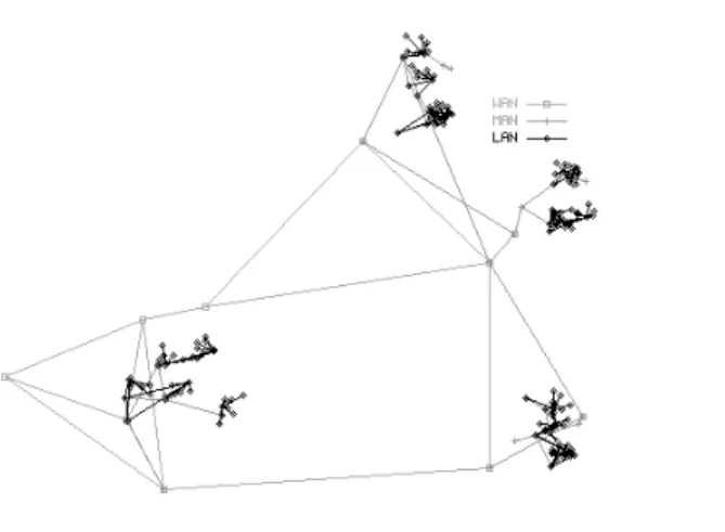
Figure 2-7: Original network topology generated by tiers. There are 180 nodes.

Figure 2-8: Visible network. Illustrates the network topology after monitors have been added and non-traversed nodes and links have been removed.

Figure 2-9: Reduced network. Series and consecutive equivalent links have been removed from the visible network.

(25)

2.3 Implementation

tiers Output (gnuplot cmd file) imm matriod correlation reduce topomap fixed network simulator Path-link Matrix Network Graph (gif image) Topology File (reduced network) Data

File Fixed m-labels

Points File Compare Graphs Visually Compare Graphs Technically Topology File (discovered network) topomap (Initial Network) (Discovered Network) Network Graph (gif image) cat parameters parameters parameters parameters Isomorphic? Yes or No

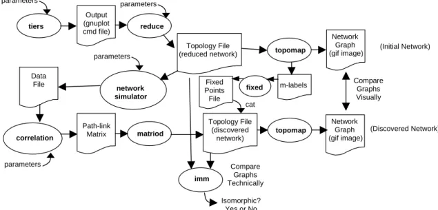
Figure 2-10: Code tool-chain. Ovals refer to programs and squares refer to files.

In Figure 2-10, we show how the various pieces of code interact. Ovals refer to programs and squares to files. Walking briefly through this chart, the tiers program generates the original network. This network is input to the reduce program that chooses monitors and removes non-traversed links and nodes, series links, and consecutive

equivalent links. The reduce program captures the ideas of section 2.2. The output of the

reduce program is a description of the reduced network, or a topology file. The network simulator then simulates a network model on the reduced network. End-to-end delay

data is recorded by the network simulator and stored in a data file. This data file is input to the correlation algorithm, which attempts to solve for the path-link matrix. Finally, the matroid algorithm reconstructs the reduced network topology using the path-link matrix. The matroid algorithm outputs the discovered network as a topology file.

On the right-hand side of the figure, the reduced network is rendered and compared with the discovered network. Topomap is a graph drawing program that draws networks in a visually appealing manner. The purpose of fix is to place the monitors in the same locations in the diagrams of the reduced network and the discovered network. We can

(26)

compare the reduced network and the discovered network visually as well as with the graph isomorphism checker, imm.

These programs were all written in C. The primary authors of these programs are:

correlation- Jason Baron fixed- Jason Baron imm- Paul Seymour matroid- Paul Seymour

network simulator- Jason Baron, Mark Garrett, Alex Poylisher reduce- Jason Baron

topomap- Bruce Siegell

The algorithm timings referred to in the remainder of this paper were all performed on a Sun Ultra 5 running the SunOS 5.7 operating system with 64MB of RAM.

(27)

Chapter 3 Non-Overlapping Congestion

In this chapter, we consider the first network model. In section 3.1, we explain the assumptions and features of the network model. Section 3.2 introduces the idea of applying a threshold to the paths’ end-to-end delay time series to produce a binary function. We find this to be a powerful technique and make use of it in solving this and subsequent network models. Section 3.3 presents two correlation algorithms—a simple algorithm that does not take some of the aspects of this network model into account and a more sophisticated algorithm that attempts to deal with these aspects. The results of testing the second algorithm are presented in section 3.4. Finally, we provide results and discussion in section 3.5.

3.1 Network Model

The network model consists of FIFO output queuing, no input queuing, and no processing delay at nodes. Therefore, there is a one-to-one correspondence between output queues and links. All links have identical bandwidth—1.55 Mbps.

The congestion aspects form the core of the model. Queues are congested by having packets of size 1250 bytes independently injected into them at a rate that is chosen from a heavy-tailed distribution*. After the injected packets have made their way to the front of the queue, they are simply discarded. The time for which a queue is injected with packets is fixed and this parameter is the congestion_length, which can be varied between

simulation runs.

*

We sample packet arrival rates from the VBR video trace used in [8]. This empirical data has a heavy-tailed distribution.

(28)

The key feature of this network model is that only one queue is being injected with packets at any given time. Queues are chosen to have packets injected into them at random. More precisely, if there are k queues and one queue has finished being injected with packets, then the probability that any one of the queues is chosen next for injection with packets is 1 k. The time between the end of one queue being injected with packets and the start of a subsequent queue being injected with packets is the controlled by the

inter_congestion_length parameter, which can be varied between simulation runs.

Monitors send time-stamped packets or probes of size 576 bytes to other monitors in a round-robin fashion. The frequency at which these packets are sent is inversely

proportional to the number of monitors. Specifically, if monitor M1 sends a probe packet to monitor M2 at time t, then monitor M1 will send its next probe packet to monitor M3 at a time that is uniformly chosen between t and t+(2 numberof monitors). Packets are not sent at fixed intervals because we would like to detect events that may be happening periodically. As the size of the network grows, we increase the frequency that monitor packets are sent in order to maintain the rate at which probes measure network

conditions. The consequence of generating probe packets in this manner is that if there are m monitors, then traffic may grow in some regions of the network by m3.

Monitors that receive probes from other monitors calculate the end-to-end delay for a particular path by subtracting the time-stamp on the packet from the time that the packet was received. The receiving monitor then records the duple data: <time-stamp on

received packet, end-to-end delay time>. Lost packets are ignored.

Two aspects of the model make finding the path-link matrix from the collected data difficult. If one could measure the underlying congestion aspects perfectly, then a

congestion event or an increase in a path’s end-to-end delay time would begin and end at

almost the same time on those paths that contain the congested queue. However, since we are probing at somewhat random intervals, increases and decreases in end-to-end delay measurements do not line up between paths perfectly in time. We consider this to be an inherent measurement difficulty. A second difficulty arises if the

(29)

to a heavy-tailed distribution, end-to-end delay times on paths that do not share any common queues may show correlation, despite the fact that only one queue is injected with packets at any given time.

Let us ignore the second difficulty for a moment. There is still a question of when to conclude that two paths share a common congestion event because of measurement uncertainty. We deal with this difficulty by applying a threshold to the end-to-end delay time series.

3.2 Applying a Threshold to the Delay Time Series

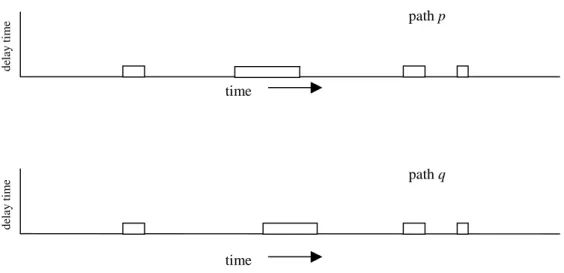
In order to decide if two paths share a common congestion event, we first apply a threshold to the end-to-end delay time series of each path. The result is a binary function that is 0 when the delay time series is below the threshold and 1 when the delay time series is above the threshold. To illustrate, the end-to-end delay time series for paths p and q are shown in Figure 3-1.

Figure 3-1: Applying a threshold. The end-to-end delay time series for paths p and q are shown with a threshold drawn on top. Note that this time series is only illustrative and is not meant to represent a recorded time series. In practice, the time series tends to be more punctuated and not as smooth as

what is illustrated. path p time de la y tim e threshold path q time de la y tim e threshold

(30)

After applying a threshold, the binary functions that result are in Figure 3-2.

Figure 3-2: Binary functions. The binary functions that result from applying a threshold to the end-to-end delay time series of paths p and q.

In practice, we set the threshold at a level such that if no queues are congested on a path then the end-to-end delay time for that path should be below the threshold value. However, if at least one link congests on a path then the paths’ end-to-end delay time should exceed the threshold value. We have set the threshold value to satisfy these properties by looking at the end-to-end delay time series. Setting the threshold in this manner certainly does not guarantee that the threshold will have its desired properties. Based upon the binary functions, we can easily specify rules as to when a common congestion event is shared between paths. A rule might be: if the starting and ending times when two binary functions take on the value of 1 are similar, then this is a shared congestion event. Therefore, paths p and q share three congestion events. They might share a fourth event. However, the starting and ending times when the two binary functions are 1 are disparate due to measurement uncertainty.

There are certainly other techniques for identifying common congestion events on two paths. For example, one might consider using a continuous correlation function. We

time path q de la y tim e time path p de la y tim e

(31)

have not explored the use of such techniques completely, but we show that applying a threshold to a delay time series is a powerful technique.

3.3 Algorithm

3.3.1 First Correlation Algorithm

Given the technique of applying a threshold to a path delay time series, a simple algorithm for determining the path-link matrix presents itself. Scan all paths over time and identify or circle the times when combinations of paths simultaneously take on the value 1. For example, a sample of the time series for the four paths p, q, r, and s is shown in Figure 3-3.

Figure 3-3: Circling algorithm. Times when only path p and path r share a congestion event are circled. If we continue circling all the unique sets of congestion events in this manner, we can

construct the path-link matrix in a straightforward manner.

Here, we have circled the three instances when only paths p and r share a congestion event. If we continue to circle congestion events in this manner, then we can easily construct the path-link matrix. The columns in the path-link matrix correspond to the columns that we have circled. Paths in a circle that have a value of 1 are 1 in the corresponding position in the path-link matrix and 0 otherwise. The key assumption is that each link in the network is traversed by a unique set of paths and therefore any two circled sets of congestion events that have the same set of congested paths must have been caused by the same link in the network. It also follows that any two circles of

path p: path q: path r: path s:

(32)

congestion events that have a different set of congested paths must have been caused by a different link in the network.

This algorithm, which we refer to as the circling algorithm, solves this congestion model to an extent. However, it does not address the two difficulties of the network model. First, if the inter_congestion_length approaches 0, it would start to become unclear as to what should be circled. Second, measurement uncertainty causes congestion events to not line up perfectly in time and thus circling becomes more difficult.

3.3.2 Second Correlation Algorithm

We now propose an algorithm that addresses the two difficulties of this model. The basic idea of the algorithm is to use pair-wise comparisons between paths that indicate whether or not two paths share a common cause of congestion. This pair-wise

comparison takes many events into consideration, instead of just a single event as in the circling algorithm. The algorithm forms groups of paths that have at least one common link by adding one path at a time to a group through pair-wise comparisons. When the algorithm terminates, the groups correspond to columns in the path-link matrix. We must be careful in constructing these groups, since if there are n paths, then there are 2n

possible groups.

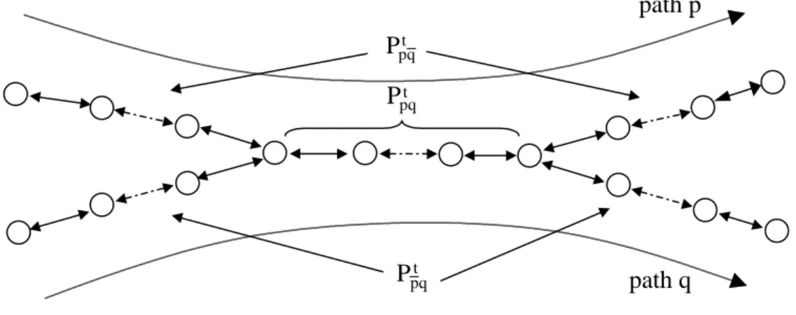
In deriving a pair-wise comparison test, we start with a model that contains two paths. Paths p and q are shown in Figure 3-4. We classify the links on these two paths as belonging to one of three categories: links on path p and not on path q, links on path q and not on path p, and finally links on both paths p and q. These three categories of links can be thought of as three causes of the congestion events that are observed on paths p and q. We represent the probability that at least one link congests in each of these three categories as: t q p P , t q p P , and t pq

P . We refer to these three probabilities as trigger probabilities, since they can be thought of as triggering congestion events.

(33)

Figure 3-4: 2-path trigger probabilities. Links that are dashed are meant to represent zero or more links. t

q p

P is the probability that at least one of the links that is on path p and not on path q congests.

t q p

P is the probability that at least one of the links that is on path q and not on path p congests. Finally, t

pq

P is the probability that at least one link of the links common to both paths p and q congests.

There are four possible outcomes that we can observe, looking at the binary functions of both paths p and q at any instant in time. Path p might be 1 or 0 and path q might be 1 or 0. To calculate an estimate of the probability of any one of these four outcomes, one can divide the total time that each one of these four outcomes occur by the total

observation time. We refer to the probability of each outcome as an observation probability. The notation that we use to designate the probability of each one of these four outcomes is: o

pq

P , if both paths’ binary functions are 1, o q p

P , if path p’s binary function is 1 and path q’s binary function is 0, o

q p

P , if path p’s binary function is 0 and path q’s binary function is 1, and o

q p

P , if both paths’ binary functions are 0.

Assuming that the trigger probabilities are independent, the relationship between the observation probabilities and the trigger probabilities is the same here as in Ratnasamy et

al. [17]. However, the underlying model that Ratnasamy uses is different from the model

here. The Ratnasamy equations are:

t q p P t q p P t pq P path p path q

(34)

t q p t q p t pq t pq o pq P (1 P )P P P = + − (3.1) ) P 1 ( P ) P 1 ( P t q p t q p t pq o q p = − − (3.2) t q p q p t pq o q p (1 P )(1 P )P P = − − (3.3) The solution of t pq

P from Ratnasamy is:

1 P P P P ) P ( P P P P P P P o q p o q p o pq o pq 2 t pq o pq o q p o q p o q p o q p o pq t pq ₊ ₊ ₋ − + + + = (3.4) If the value of t pq

P is significant, we conclude that two paths share a common congestion cause. We refer to testing two paths for a common cause as the t

pq P test.

This pair-wise test addresses the two difficulties of the model as follows. First, it addresses the issue of queues being simultaneously congested because the model assumes that triggering events can happen simultaneously. Second, we assume that the

measurement uncertainty is short relative to the duration of the congestion_length and thus the trigger probability estimates are not significantly affected. We have been a bit brief about this model because we will return to it in greater detail in chapter 4.

Assume that for two paths, a and b, the value of the t pq

P test is significant and

therefore we conclude that paths a and b share a common congestion cause. We form the group(a,b) and associate the intersection of path a’s binary function and path b’s binary function with this group. The intersection of two binary functions is 1 when both binary functions are 1 and 0 otherwise. The result of the intersection operation is a binary function that provides some information as to what congestion events the two paths have in common.

Now, we could test whether path c shares a common congestion cause with group(a,b) by applying the t

pq

P test again, treating the intersected binary function formed from paths

(35)

If the t pq

P test is not significant, then we continue to grow the group(a,b) by trying the t pq P test with additional paths. However, if the t

pq

P test is significant then we form the

group(a,b,c) and associate the intersection of the binary functions of path a, b, and c with this group.

In deciding whether or not to keep the group(a,b), we subtract the binary function associated with group(a,b,c) from the binary function associated with the group(a,b). The subtraction operation is 1 when the minuend is 1 and the subtrahend is 0 and 0 otherwise. If we determine that there is a significant binary function left, meaning that there are a number of congestion events yet to be explained, then group(a,b) is kept. Otherwise, if this binary function is not significant, we delete the group(a,b). We also define a unite operation on two binary functions that is 1 when at least one binary function is 1 and 0 otherwise. Based upon the intersection, subtraction, and unite operation, and the two significance tests (the t

pq

P test and the test for detecting if significant congestion events remain), we construct the algorithm in

(36)

Figure 3-5: Pseudocode of the correlation algorithm.

Input:

NUMBER_OF_PATHS; the number of paths

PATH_BINARY_FUNCTIONS : Array (Binary Function); PATH_BINARY_FUNCTION[i] is the binary function of path i

Output:

PATH_LINK_MATRIX: 2D Array; x_i,_j=

CORRELATE () {

processed_events : Binary Function; initially contains no Events unexplained_events : Binary Function

for path = 1 to NUMBER_OF_PATHS

unexplained_events = PATH_BINARY_FUNCTIONS[path] subtract processed_events

if unexplained_events is significant

BREAK-UP(unexplained_events, path, (path+1))

processed_events = processed_events unite PATH_BINARY_FUNCTIONS[path]

}

BREAK-UP(matching_events: Binary Function, group_paths : set of paths in this group, lowest_candidate_path : minimum path that we try to add to this group) {

intersect : Binary Function

for path = lowest_candidate_path to NUMBER_OF_PATHS

if P_pqt test between matching_events and PATH_BINARY_FUNCTIONS[path] is significant intersect = matching_events intersect PATH_BINARY_FUNCTIONS[path]

matching_events = matching_events subtract intersect BREAK-UP(intersect, group_paths ∪ path, (path+1)) if matching_events is not significant

return

append 1 column to PATH_LINK_MATRIX

for all i ∈ group_paths

PATH_LINK_MATRIX[ i, numOfColumns(PATH_LINK_MATRIX)] = 1

}

1 if path i contains link j 0 otherwise

(37)

The input to the algorithm is the NUMBER_OF_PATHS, and the

PATH_BINARY_FUNCTIONS. For convenience, we assume that the paths are numbered 1 through the NUMBER_OF_PATHS. Therefore, we index into the PATH_BINARY_FUNCTIONS array with a number between 1 and

NUMBER_OF_PATHS.

The algorithm recursively forms a tree in a depth first manner. A group is associated with each node in the tree. Associated with a group are a set of paths, group_paths, a binary function, matching_events, and the lowest_candidate_path. We attempt to add all paths with a number greater than or equal to the lowest_candidate_path number to the group.

The procedure BREAK-UP is called on the node in the tree where we are progressing. The group associated with this node is the current group. The BREAK-UP procedure successively tries the t

pq

P test between the binary function associated with the current group, matching_events, and the binary function for all paths with a path number greater than the lowest_candidate_path. If this test is significant at any point, we form a new group.

The paths associated with the new group include all the paths in the current group and the path that was being tried when the t

pq

P test returned a significant result. Let us assume that we were trying to add path i, when the t

pq

P test returned a significant result. The binary function associated with the new group is formed via the intersection of the binary function that is associated with the current group and the binary function of path i. We also subtract the binary function that we have just associated with the new group from the current group’s binary function. We call BREAK-UP next on this new group where we have set the new group’s lowest_candidate_path to (i + 1).

Control is returned from the BREAK-UP procedure to the parent node in the tree in two cases. First, if the binary function associated with the current group is no longer significant. Second, when we have finished trying to add all paths greater than or equal to the lowest_candidate_path number to the current group and the congestion events

(38)

associated with the current group are significant. In this second case, we have identified a link and therefore we add a column to the path-link matrix.

The algorithm is initialized in the procedure CORRELATE by calling BREAK-UP on initial groups. We form one initial group for each path, initializing the set of paths that we associate with each initial group to contain that single path. The

lowest_candidate_path is set to one more than the path number that is associated with

each initial group. We initialize the binary function for the initial group that contains only the path i by subtracting all of the binary functions that have a path number that is less than i from path i’s binary function. This is analogous to subtracting the new group’s binary function from the current group’s binary function during a call to BREAK-UP. The root node of the tree can be thought of as containing all of the congestion events on all of the paths. By subtracting the binary functions of all paths that are numbered less than i from the binary function of path i, we are subtracting all congestion events that we have already explained.

3.3.3 Time and Space Complexity

We analyze the running time of the second correlation algorithm, assuming that the significant tests are always correct. Let:

M ≡ number of monitors

P ≡ number of paths = M ×(M – 1) L ≡ number of links

N ≡ simulation length

The number of leaves in the tree that is formed is L and the number of nodes between the root and a leaf is at most P. Therefore, there are O(PL) nodes in the tree. We can also associate at most a single intersection and subtraction operation with each node in the

(39)

tree. The t pq

P test takes time proportional to N. At each node in the tree we perform the t

pq

P test at most O(P) times. Therefore, we bound the running time of this algorithm as O(P2LN).

3.3 Results and Discussion

The algorithm performed well when the inter_congestion_length was large. However, as the inter_congestion_length was decreased towards zero, the algorithm did not

necessarily find the correct path-link matrix. Here, we only present the largest network that was solved with the algorithm.

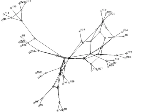
The reduced network has 30 monitors, 36 internal nodes, and 160 links. The correlation algorithm solved for the correct path-link matrix in 20 seconds using 80 minutes of simulated traffic. The congestion_length was 10 seconds and the

inter_congestion_length was 5 seconds. The reduced network is shown in Figure 3-6 and

the discovered network in Figure 3-7. The two networks are identical except for 8 split nodes that are mostly in the interior of Figure 3-7. When we show an example or data about the topology discovering algorithms, the correlation algorithm always finds the correct path-link matrix, unless otherwise noted. The split nodes are the result of the matroid algorithm.

(40)

Figure 3-6: Reduced network. 30 monitors, 36 interior nodes, and 160 links.

Figure 3-7: Discovered network. Network discovered by the matroid and correlation algorithms. This network is identical to the reduced network except for 8 split nodes. These split nodes appear as

two nodes that are slightly offset. By comparing Figure 3-7 with Figure 3-6 the split nodes can be identified.

(41)

We have developed an algorithm that attempts to account for the difficulties of the non-overlapping congestion model. The algorithm performed well when the

inter_congestion_time was large. However, as the inter_congestion_time approached 0

the correct path-link matrix was elusive. Despite the algorithm’s shortcomings, the algorithm begins to capture ideas of how to deal with overlapping congestion events that are due to different queues and measurement uncertainty.

One problem with the algorithm is that the meaning of the t pq

P test is unclear, when one of the binary functions is the result of intersected and subtracted binary functions. Another problem is deciding when the t

pq

P test is significant and when a significant number of congestion events remain in a binary function.

The subsequent network model has no measurement uncertainty. Instead, we focus on the difficulty that is caused when queues simultaneously congest. Thus, we isolate one of the difficulties of this network model.

(42)

Chapter 4 Overlapping Congestion in Discrete Time

The overlapping congestion in discrete time network model both simplifies and

complicates aspects of the non-overlapping congestion network model. We introduce the overlapping congestion in discrete time network model in section 4.1. Section 4.2

presents a probability framework that forms the basis for the algorithm that is presented in section 4.3. Finally, in section 4.4, we provide results and discussion.

4.1 Network Model

In this network model, time is divided into discrete intervals. There is no input queuing at nodes, only output queuing. Therefore, there is a one-for-one correspondence between queues and links.

In each interval, each queue either does or does not congest. The probability that a queue congests in an interval is fixed at the same value for all intervals and is

independent of all other queue congestion. Different queues may have different probabilities of congestion or congestion rates. We assume that the congestion rate on each link is greater than zero and that the congestion rate on the least congested link in the network is known. When a queue congests during a time interval n, all paths that traverse this queue are congested or high during time interval n. Therefore, a path p is congested during the time interval n if and only if at least one queue on path p congests during time interval n.

We can use a binary function to represent the congestion that occurs on a path over time. This binary function is 1 in time interval n if the path is congested and 0 otherwise. We refer to this binary function as a path’s end-to-end delay time series.

(43)

This congestion model abstracts away some difficulties that we encountered in solving the non-overlapping model. Most importantly, all paths that contain a congested queue are all high simultaneously. There are no longer questions about whether or not

congestion is temporally related. Thus, the measurement uncertainty of the non-overlapping model is no longer troublesome.

However, simultaneously congesting queues introduces new difficulties in

determining the paths that traverse each link in a network. For instance, the sets of links on two separate paths in a network may be disjoint. However, queues on both of these paths might congest simultaneously. Consequently, there would appear to be a link in the network traversed by both paths. In order to begin to reason about this model, we

introduce a probability framework in the next section.

4.2 Probability Analysis

4.2.1 Observation Probability

An observation probability is defined as the probability that specific paths are or are not congested. In order to formalize this notion, we introduce some random variables:

   λ = λ otherwise 0 n time at congested is link if 1 ] n [ x (4.1)

Next, we define a random variable that is 1 if at least one link on path p is congested during interval n and 0 otherwise.

   ∃λ∈ = = λ otherwise 0 1 ] n [ x that such p if 1 ] n [ y_p (4.2)

(44)

Now, we define a random variable that takes on the value 1 if from among a certain set of paths, some of these paths are congested, while the remaining paths in the set are not congested:    = = = = = otherwise 0 0 ] n [ y , 1 ] n [ y , 0 ] n [ y , 1 ] n [ y 1 ] n [ z_p_,_q_,_r_,_s p q r s (4.3)

Note that a path without a bar above it refers to a path that is congested while a path with a bar above it refers to path that is not congested. We introduce the observation

probability as: ] 1 ] n [ z Pr[ P_po_,_q_,_r_,_s = _p_,_q_,_r_,_s = (4.4) We let o i e

P represent a general observation probability, where e is the set of excluded paths and i is the set of included paths. A path that is excluded from the observation probability is not congested and thus has a bar above it. A path that is included in the observation probability refers to a path that is congested and does not have a bar above it. A path that does not appear in the subscript of an observation probability is ignored. In order to be clear about the meaning of an observation probability, we imagine that the end-to-end delay time series for paths p, q, r, and s are as shown in Figure 4-1.

Figure 4-1: Calculating an observation probability. The binary functions of paths p, q, r, and s are shown. We have circled the times when paths p and r are congested and paths q and s are not congested. By dividing the number of times we have circled this event, 3, by the simulation length,

25, we estimate P_po_,_q_,_r_,_s. path p: path q: path r: path s: 1 5 10 15 20 25

(45)

An estimator of

P

_po_,_q_,_r_,_sis: N z Pˆ N 1 p,q,r,s o s , r , q , p =

∑

(4.5)

Therefore, in the example of Figure 4-1, an estimate of

P

po,q,r,s is 3 25 or 0.12.

4.2.2 Trigger Probability

Estimates of the observation probabilities are calculated from the time series. However, these estimates are not informative as to individual link congestion rates. In order to estimate individual link congestion rates, we introduce the trigger probability. A path p consists of a set of links. If all of the links in a given network are contained in the set U, then the complement of the set of links that constitute path p is defined as all of those links contained in the set U and not in the set p. We refer to this set of links, denoted p , as path p’s complementary links. The intersection of path p’s links and path

q’s complementary links is also a set of links. Therefore, thinking of a path as a set of

links, we adopt the following notation:

s r q p s r q p = ∩ ∩ ∩ (4.6) We define a random variable that is 1, if there is congestion on at least one link in the set that is defined by the intersection of certain paths’ links and certain paths’

complementary links.    = ′ otherwise 0 n time at congested is s r q p set the in link one least at if 1 ] n [ z_p_q_r_s (4.7)

(46)

The trigger probability is defined as: ]] 1 ]] n [ z Pr[ P_pt_q_r_s = _p′_q_r_s = (4.8) We let t i e

P denote a general trigger probability. A path that is included in the trigger probability does not have a bar above it and refers to the set of links on that path. A path that is excluded from the trigger probability has a bar above it and refers to that path’s complementary links. A path that does not appear in a trigger probability subscript is

ignored.

We assume that each link in the network is traversed by a unique set of paths. Therefore, we characterize a link by specifying whether or not each path traverses that link. Therefore, if there are n paths, then there are (2n-1)* possible links. Some of the possible links are in the network and are true links, while some of the possible links are not in the network and are false links.

Through the intersection of the sets of links referred to by included and excluded paths, a trigger probability specifies a set of links that are truly in the network or the empty set. Assuming that we have n paths and we include or exclude each path in a trigger probability (we do not ignore any paths), then the trigger probability is fully

specified and must refer to an individual link. This individual link could either be a true

link or a false link. If it is a false link then the intersection of the sets of links referred to by the included and excluded paths is the empty set. There are (2n – 1)** fully specified trigger probabilities that correspond to each of the possible links.

Assume that each link in the network congests with a probability greater than zero and that we observe the network for an infinite amount of time. Also, assume that we can calculate the value of all fully specified trigger probabilities. The trigger probabilities that refer to true links would have a value greater than zero, while the trigger probabilities that refer to false links would have a value of zero. The fully specified trigger

*

We do not consider the link that is not traversed by any path.

(47)

probabilities that refer to false links specify an empty set of links and therefore the probability of congestion is zero. In practice, trigger probabilities are not necessarily equal to their limiting value because of finite sample sizes. Although we do not observe the trigger probabilities directly, we can relate the trigger probabilities to the observation probabilities.

4.2.3 Relating Trigger Probabilities to Observation Probabilities

The sample network shown in Figure 4-2 has 5 monitors, 20 paths and 24 links. Let us relate the trigger probabilities to the observation probabilities for paths p and q, as shown.

Figure 4-2: Relating trigger probabilities to observation probabilites for paths p and q.

path p path q L2 L3 L4 L5 L7 L8 M1 M5 M2 M3 M4 L1 L6

(48)

Using the random variables that we have defined: ] 1 ] n [ z Pr[ P_po_,_q = _p_,_q = ] 0 ] n [ y , 0 ] n [ y Pr[ _p = _q = =

The probability that there is no congestion on either path p or path q is:

] 0 ] n [ x ], n [ x , 0 ] n [ x , 0 ] n [ x , 0 ] n [ x , 0 ] n [ x , 0 ] n [ x , 0 ] n [ x Pr[ 8 7 6 5 4 3 2 1 = = = = = = = = _λ _λ _λ _λ _λ _λ _λ _λ

Making use of the fact that links congest independently:

] 0 x , 0 x , 0 x Pr[ ] 0 x , 0 x , 0 x , 0 x Pr[ ] 0 x Pr[ 8 7 6 5 4 3 1 2 = ⋅ = = = = ⋅ = = = = _λ _λ _λ _λ _λ _λ _λ _λ

Finally, realizing that these three sets of links can be written as the following path intersections, we have: ) P 1 )( P 1 )( P 1 ( t q p t q p t pq − − − =

This equation relates an observation probability to three trigger probabilities. For two paths, there are three trigger probabilities of interest: t

pq P , t q p P , and t q p P . We are only interested in links that are on either path p or path q and therefore do not consider the trigger probability, t

q p

P . Expressing the observation probabilities P and _po P in terms of_qo the three trigger probabilities of interest yields two more equations, giving us a total of three equations in three unknowns:

(49)

) P 1 )( P 1 )( P 1 ( P t q p t q p t pq o q p = − − − (4.9) ) P 1 )( P 1 ( P t q p t pq o p = − − (4.10) P (1 P )(1 P ) t q p t pq o q = − − _(4.11) We refer to equations (4.9), (4.10), and (4.11) as the 2-path equations. The form of the 2-path equations is similar to equations derived by Ratnasamy and McCanne [17]. Using the notation introduced here, the Ratnasamy equations can be written as:

t q p t q p t pq t pq o pq P (1 P )P P P = + − (4.12) ) P 1 ( P ) P 1 ( P t q p t q p t pq o q p = − − (4.13) t q p q p t pq o q p (1 P )(1 P )P P = − − (4.14) The 2-path equations differ from the Ratnasamy equations in an important respect. Although, observation probabilities are only on the left-hand sides and trigger

probabilities only on the right-hand sides of both sets of equations, the 2-path equations only involve observation probabilities that are the result of an absence of triggering events. In the Ratnasamy equations, observation probabilities reflect both the absence as well as a presence of triggering events. The right-hand sides of equations (4.9), (4.10), and (4.11) only multiply together inverse trigger probability terms that are of the form: (1 - t

i e

P ). On the other hand, the Ratnasamy equations contain terms of the form (1 - t i e P ) and ( t i e

P ) combined in a more complex manner. Although the model used in deriving the 2-path equations differs from the model used by Ratnasamy, the trigger probabilities are equivalent*.

The 2-path equations are solved for the trigger probabilities as follows. The terms t q p P and t q p

P are solved for by dividing equation (4.9) by equations (4.11) and (4.10),