Re-examination of M₂,₃ atomic level widths of elements 69 ≤ Z ≤ 95 and double K-shell ionization of A1 induced by photon and electron impact

(1)

Université de Fribourg (Suisse)

Re-examination of M

2,3

atomic level widths

of elements 69 ≤ Z ≤ 95

and

Double K-shell ionization of Al

induced by photon and electron impact

THESE

Présentée à la Faculté des Sciences de l’Université de Fribourg (Suisse) pour l’obtention du grade de Doctor rerum naturalium

Karima Fennane

du Maroc

Numéro de la thèse: 1597

Imprimerie Saint-Paul, Fribourg 2008

(2)

Fribourg, le 18 Mars 2008

Le directeur de thèse : Le doyen :

(3)

α

Energy ... 87 4.1.2 _K h 2

α

line width ... 88 4.1.3 K hL 2

α

satellite ... 88

4.2 Results from electron measurements... 89

4.3 Double K-shell photo-ionization probabilities ... 90

4.4 Comparison between the double to single K-shell ionization cross sections . produced by photon and electron impact... 93

5. Concluding remarks and future perspectives ... 99

Bibliography ... 101

Acknowledgements... 111

Curriculum Vitae ... 113

(5)

Abstract

The present Ph.D. thesis contains two different research projects in Atomic Physics, whose common denominator is high-resolution x-ray emission spectroscopy. The first project belongs to the field of x-ray transition metrology and concerns the determination of the M2 (3p1/2) and

M3 (3p3/2) level widths of elements with atomic numbers in the region 69≤Z≤95. The second

part is devoted to the investigation of double K-shell ionization of metallic aluminium induced by photon and electron impact.

The x-ray transition metrology project of the L1M2 and L1M3 x-ray transitions widths for

elements ranging from Thulium (Z=69) to Americium (Z=95) was incited by the work of Professor J. L. Campbell from the University of Guelph, Canada. Campbell et al. had assembled recently a large number of experimental data from which they derived an internally consistent set of level widths for the K shell to the N7 subshell for all elements across the

periodic table [At. Data Nucl. Data Tables 77, 1 (2001)]. In the plot representing the variation of the M3 level width as a function of the atomic number Z, the authors found a hump around

Z=83 which is not predicted by the DHS (Dirac-Hatree-Slater) theoretical calculations. Campbell had suspected the L1M3 transitions widths measured by J.N. Cooper [Phys. Rev. 65,

155 (1944)], which were the main source of his recommended M3 level widths in the Z region

75≤Z≤92, to be too high and had suggested that new high resolution measurements of these transitions would be useful to clarify the Z dependence of the M3 level width. Furthermore, as

Campbell’s M2 recommended level widths in this Z region are also based on the L1M2

transition widths of Cooper, a new set of measurements for the L1M2 transitions widths was

called for.

The measurements were performed at the University of Fribourg by means of two different high resolution crystal spectrometers. Elements up to 77Ir were measured with a reflection-type

von Hamos crystal spectrometer. As this instrument cannot be used efficiently for photon energies above 11 keV, elements with higher atomic numbers were measured with a transmission-type DuMond crystal spectrometer. The fluorescence x-ray emission was produced by irradiating the samples with the bremsstrahlung of an x-ray tube.

From the linewidths of the measured L1M2 and L1M3 x-ray transitions of 69Tm, 70Yb, 71Lu, 73Ta, 74W, 75Re, 77Ir, 81Tl, 83Bi and 95Am an accurate set of M2 and M3 level widths was

(6)

results are 3-5 times more accurate than the former existing data. The observed abrupt changes of the M2,3 level widths versus atomic number Z could be explained satisfactorily by the

cut-offs and onsets of the M2M4N1, respectively M3M4N3,4,5 and M3M5N2,3 CK (Coster-Kronig)

transitions deduced from the Z+1 semi-empirical rule.

As a spin-off result of this study, precise L1M2 and L1M3 transition energies were obtained

for the investigated elements. A very good agreement with MBPT theoretical values was found.

The second project concerns the investigation of double K-shell ionization of metallic aluminium induced by photon and electron impact. Two objectives were set for this project. The first was to overcome the lack of experimental data on double K-shell ionization in light elements. The second was to investigate the energy dependence of both the photon- and electron-induced double to single 1s ionization cross section from threshold to the expected broad maximum in order to better understand the mechanisms by which the double 1s vacancy production is achieved in each case. The x-ray synchrotron based measurements of the double to single photoionization cross sections for Al represent the first of the kind.

The experimental method consisted to measure the Kα hypersatellites spectra resulting from the radiative decay of the double K-shell vacancy states by means of high resolution x-ray emission spectroscopy using the Fribourg Bragg type von Hamos crystal spectrometer. Measurements of the photon-induced spectra were carried out at the x-ray microscopy beam line ID21 at the European Synchrotron Radiation Facility (ESRF), Grenoble, France, whilst those of the electron-induced spectra were performed at the University of Fribourg. The

(7)

recoil momentum in case of photo-absorption and projectile impact ionization. The threshold energy for the production of double K-shell vacancies was estimated to be comprised between 3235 eV and 3318 eV in the case of photoionization and at about 4.6 keV for the electron-induced ionization.

The energy and linewidth of the Kα2 hypersatellite x-ray emission line were also

determined. Both the photon and electron impact data lead to consistent results of 1610.38(10) and 1610.37(11) respectively for the Kα2 hypersatellite transition energy and 1.88(10) eV and

1.87(17) eV for the linewidth. No trace of the Kα1 ([1s-2] → [1s-12p3/2-1]) hypersatellite

transition was detected in the measured x-ray spectra due the prevailing LS coupling scheme for light elements.

Moreover, it was found that the evolution of the measured double to single K-shell photoionization cross section with photon energy deviates considerably from the predictions of the Thomas model based on the time-dependent perturbation theory and accounting solely for the shake process. These findings evince the relative importance of the electron-electron scattering contribution to the double 1s ionization for Al. The PKK value in the maximum of

the double ionization cross-section was compared to the Z-dependence of PKK reported by

Kanter et al. in [Phys. Rev. A 73, 062712 (2006)]. A good agreement with the value deduced from the proposed scaling law 1/Z1.6 for neutral elements was obtained.

(8)

dont le dénominateur commun est la spectroscopie X de haute résolution. La première étude s’inscrit dans le domaine de la métrologie des rayons X et concerne la détermination de la largeur des niveaux atomiques 3p1/2 (sous-couche M2) et 3p3/2 (sous-couche M3) des éléments

ayant un numéro atomique 69 ≤ Z ≤ 95. La deuxième étude concerne la double ionisation K de l’aluminium produite par l’impact de photons et d’électrons.

Le projet de métrologie de rayons X dont l’objectif était de déterminer les largeurs naturelles des sous-couches atomiques M2 et M3 nous a été suggéré par le professeur J. L.

Campbell de l’Université de Guelph, Canada. Campbell et Papp ont publié récemment une synthèse des résultats expérimentaux concernant les largeurs naturelles de transitions atomiques dont ils ont extrait un ensemble auto-consistant des largeurs des couches atomiques K à N7 de tous les éléments du tableau périodique [At. Data Nucl. Data Tables 77, 1 (2001)].

Dans le graphique représentant la variation de la largeur de la sous-couche M3 en fonction du

numéro atomique Z, les auteurs ont observé une bosse centrée autour de Z = 83 qui n’est pas prédite par les calculs théoriques DHS (Dirac-Hartree-Slater). Les valeurs recommandées par Campbell et Papp pour les largeurs du niveau 3p3/2 dans la région 75 ≤ Z ≤ 92 ayant été

extraites principalement des largeurs des transitions L1M3 mesurées par J. N. Cooper plus de

50 ans auparavant [Phys. Rev. 65, 155 (1944)], Campbell a suggéré que ces anciennes valeurs étaient peut être surestimées et que de nouvelles mesures de haute résolution des transitions L1M3 seraient donc très utiles pour clarifier la dépendance en Z des largeurs M3. Comme les

valeurs recommandées par Campbell et Papp pour la largeur du niveau atomique M2 dans la

(9)

A partir des largeurs mesurées des transitions L1M2 et L1M3 des éléments 69Tm, 70Yb, 71Lu, 73Ta, 74W, 75Re, 77Ir, 81Tl, 83Bi et 95Am et en utilisant les largeurs du niveau atomique L1

déterminées récemment par Raboud et al. [Phys. Rev. A 65, 022512 (2002)], des résultats précis et fiables concernant les largeurs naturelles des sous-couches M2 et M3 ont été obtenus.

De surcroît, la nouvelle base de données pour les largeurs M2,3 déduite de nos mesures a été

étendue à 80Hg, 90Th et 92U en utilisant les résultats de mesures des transitions L1M2,3

effectuées précédemment par notre groupe. Nous avons comparé nos résultats avec les valeurs recommandées par Campbell et Papp et avec d’autres valeurs expérimentales et théoriques reportées dans la littérature. D’une manière générale, les largeurs M2,3 obtenues dans ce travail

sont plus grandes que celles de Campbell et Papp mais plus petites que les valeurs prédites par des calculs théoriques basés sur le modèle de particules indépendantes. Nos résultats sont aussi 3-5 fois plus précis que les quelques résultats antérieurs existants. Les abrupts changements observés dans les graphes représentant la variation des largeurs M2 et M3 en fonction du

nombre atomique Z ont pu être expliqués de façon satisfaisante par le fait que les transitions Coster-Kronig M2M4N1, respectivement M3M4N3,4,5 et M3M5N2,3, deviennent soudainement

interdites ou au contraire permises pour certains éléments. La plupart des valeurs Z pour lesquels ces sauts dans les largeurs M2,3 apparaissent ont pu être expliquées par la règle

semi-empirique Z+1.

Des mesures de ce premier projet, nous avons également pu extraire un ensemble d’énergies précises et fiables pour les transitions L1M2, et L1M3 des 10 éléments énumérés ci-dessus. Un

excellent accord a été trouvé entre nos énergies expérimentales et les valeurs théoriques prédites par des calculs MBPT (many body perturbation theory).

Le deuxième projet est une étude de la double ionisation K de l’aluminium métallique produite par l’impact de photons et d’électrons. Deux objectifs avaient été ciblés pour cette étude. Le premier visait à combler le manque de données expérimentales concernant la double ionisation K des éléments légers. Le deuxième but était d’étudier la dépendance en énergie du rapport des sections efficaces d’ionisation double et simple de la couche K depuis le seuil de production de doubles lacunes 1s jusqu’à la région du « broad maximum ». Ce deuxième objectif revêtait une importance particulière pour mieux comprendre les mécanismes par lesquels la double ionisation K est produite, aussi bien dans le cas du bombardement de l’échantillon par un faisceau d’électrons que dans celui de la photo-ionisation. On mentionnera ici qu’aucune mesure du rapport des sections efficaces de photo-ionisation double et simple de la couche K de l’aluminium n’a été effectuée avant cette thèse.

La méthode expérimentale adoptée a consisté à mesurer les spectres des transitions hypersatellites Kα résultant de la désexcitation radiative des états doublement ionisés 1s-2_{. Les}

(10)

diagrammes ( [1s-1_{] → [2p}-1_{]). Les mesures ont été effectues pour des énergies de faisceau}

comprises entre 3122 eV et 5451 eV pour les photons et entre 4 keV et 20 keV pour les électrons.

Les dépendances en énergie des rapports PKK obtenus avec les photons et les électrons ont

été comparées. Nous avons trouvé que la valeur maximale du rapport était de 9.81⋅10-5 _{dans le}

cas du bombardement d’électrons alors que pour la photo-ionisation une valeur maximale bien supérieure de 1.65⋅10-3_{a été obtenue. La différence a été expliquée par le transfert de quantité}

de mouvement sur l’ion résiduel, lequel transfert n’est pas le même dans les deux types de collisions. L’énergie de seuil pour produire une double ionisation K dans l’aluminium a pu être déduite des mesures. Elle est d’environ 4.6 keV dans le cas des électrons et comprise entre 3235 eV et 3318 eV dans celui du rayonnement synchrotronique.

Nous avons aussi déterminé l’énergie et la largeur naturelle de la transition hypersatellite Kα2.Des valeurs consistantes de 1610.38(10) et 1610.37(11) pour l’énergie, et de 1.88(10) eV

et 1.87(17) eV pour la largeur, ont été obtenues à partir des mesures effectuées, respectivement, avec les faisceaux de photons et d’électrons. Par contre, aucune trace de la transition hypersatellite Kα1 ([1s-2] → [1s-12p3/2-1]) n’a été détectée dans nos mesures. Ceci

n’est cependant pas surprenant car cette transition est interdite par les règles de sélection électriques dipolaires dans le modèle de couplage LS, lequel s’applique aux éléments légers comme l’aluminium.

Nos mesures ont aussi montré que la variation du rapport PKK en fonction de l’énergie des

(11)

Part I:

Re-examination of M

2,3

atomic level

widths of elements

69 ≤ Z ≤ 95

(12)

1.1 Motivation

Some years ago Campbell and Papp [1] presented an extensive set of K to N7 atomic level

widths for all elements across the periodic table, based upon a large number of literature experimental data. Their recommended M2 and M3 level widths were derived mostly from

XPS (X-ray Photo-electron Spectroscopy) measurements for light elements and XES (X-Ray Emission Spectroscopy) measurements for elements above Z=54. For the XES measurements, Campbell and Papp extracted the M2 and M3 level widths mostly from the L1M2 and L1M3 line

width measurements of Salem [2] and Cooper [3], assuming for the L1 level widths their own

recommended values [1] (see Fig.1).

More recently Raboud et al. [4] determined the L1 atomic level width for several elements

with atomic numbers 62 ≤ Z ≤ 83 from high-resolution XES measurements of the quadrupole-allowed (E2) transitions L1M4,5, assuming for the M4,5 level widths the values recommended

by Campbell and Papp [1]. A fairly good agreement with Campbell’s recommended L1 level

widths was found, except in the lanthanide region (57 ≤ Z ≤ 70) where a large discrepancy was observed. This discrepancy was explained by a splitting effect of the L1 subshell resulting

from the coupling in the initial excited state of the 2s electron spin with the total spin of the open 4f level. This splitting effect resulting in an increase of the L1 level width that was not

considered in the compilation of Campbell and Papp, it was concluded by Raboud et al. that the M widths reported in [1] for the lanthanide region were too big. In other words, the

(13)

3 4 5 6 7 8 9 10 11 12 13 50 60 70 80 90 M3 width [eV] Z

Fig. 1: (taken from Ref. [1]): Width of the M3 level width versus atomic number

Z. Experimental data were extracted from XES measurements using the following symbols: □ Ref. [2], ∆ Ref. [3], ○ Ref. [6], ◊ Ref. [7], + Ref. [8], ● Refs. [9, 10]. The dashed dotted line represents the independent particle model calculations of Perkins et al [11], the solid line the recommended values of Campbell and Papp [1].

agreement with the new data of Raboud [4] and that both sets of values were significantly lower than the L1 level widths obtained from the L1N2,3 XES measurements of Cooper [3]

from which his L1 level widths in the region 73 ≤ Z ≤ 81 were mainly determined, using for

the N2,3 his own recommended values. Suspecting the widths of the L1M2,3 transitions

measured by Cooper to be also overestimated, Campbell eliminated from his data base the M3

level widths derived from these old measurements. Using then only the values determined from the newest L1M3 XES measurements [6, 7, 8, 9, 10] and the L1 widths from Refs. [4, 5],

he found that, as anticipated, there was no hump in this Z region of the M3 plot but merely a

smooth rise [12]. However, as these new XES data were scarce and strongly scattered, he suggested to perform a new series of modern XES measurements in order to obtain a more reliable data base for the M3 level width in the region 75 ≤ Z ≤ 92.

Following Campbell’s suggestion, we undertook to perform a series of high-resolution XES measurements of the L1M3 transitions of 69Tm, 70Yb, 71Lu, 73Ta, 74W, 75Re, 77Ir, 81Tl, 83Bi and 95Am. As the single available L1M2 XES measurements in the region 75 ≤ Z ≤ 81 were again

those of Cooper, we decided to include in our measurements the L1M2 transitions.

Furthermore, our experimental M2,3 data set was extended to 80Hg, 90Th and 92U, using former

(14)

sum of all decay probabilities. Neglecting the most improbable de-excitation modes, the width of a vacancy state is then given by the sum of the radiative, Auger and Coster-Kronig widths:

Γ =Γ_R +Γ_A+Γ_CK. (1)

Auger transitions are radiationless transitions in which the primary vacancy is filled by an electron from a higher shell with simultaneous ejection of an outer shell electron. Coster-Kronig transitions (CK) are particular Auger transitions in which at least one vacancy in the final state belongs to the same shell as the vacancy in the initial state. For instance, the Auger transition L1L3M5 is a CK transition since there is one hole in the L-shell in the initial and final

states. It should be noted that in equation (1) the CK width is excluded from the definition of the Auger width. The sum of the CK and Auger widths is sometimes named radiationless width in the literature. The probability that a vacancy in the shell S (S = K, L, M,…) becomes filled through a radiative decay is given by the fluorescence yield ωS defined by:

S S , R S _Γ Γ ω = , (2)

where ΓS and ΓR,S represent the total width, respectively the total radiative width, of the shell S. Note that the total decay probability WS of the S vacancy and total radiative decay probability WR,S are related to the parent widths by:

[ ]

h eV s W_S −1 =ΓS and

[ ]

h eV s W_R_,_S −1 =ΓR,S , (3) with _h=6.582119⋅10−16

[

eV⋅s

]

(15)

In the x-ray absorption process, an atomic electron is transferred from a given atomic state to an empty bound state or to the continuum. Since there are a multitude of possible final states, the analysis of absorption spectra is generally difficult and does not lead to precise results. When the energy of the incoming photon is sufficiently high to ionise the target atom, one can investigate the energy spectra of the ejected photo-electrons (XPS) or decay products of the ionized atoms, namely the energy spectra of the Auger electrons (AES) or x-ray transitions (XES).

The XPS technique is a direct way to measure the atomic level widths since the photo-electron energy distributions reflect the widths of the states in which the atomic vacancies were produced. This technique requires, however, the use of γ-rays or monochromatic synchrotron radiation to avoid the broadening of the photo-electron line widths as a result of the energy scattering of the photon source. Ultra-high vacuum is also needed to avoid the re-absorption of the low energy photo-electrons. Furthermore, the XPS technique is extremely sensitive to the sample surface which should be extremely clean. The same conditions (monochromatized photon source, ultra-high vacuum and ultra-clean target surfaces) should be fullfilled in AES. In addition this technique has the disadvantage that the measured line widths reflect the combined effects of the widths of the three atomic levels involved in the considered Auger transition. Finally, XPS and AES spectra of solids are also influenced by phonon excitations which are generally considered to give a Gaussian broadening to the measured spectra (see Ref. [14] and references therein).

In XES, the measurements and spectra analysis are easier to perform, since this technique is less sensitive to the sample surface contamination and the measured spectra do not reflect the energy spread of the irradiation source, nor the energy losses of the incoming and outgoing particles. The spectra are neither affected by phonon excitations. However, here again, the measured line widths contain the contribution of the widths of the two atomic levels involved in the considered x-ray transition. In any of these spectroscopic methods, multi-ionization of the target atoms can lead to broadenings or asymmetries of the measured lines. This effect can be reduced by a proper choice of the irradiation source. In this respect, photon sources are particularly appropriate, multi-ionization being only possible via weak secondary mechanisms such as shake or TS1 processes.

Finally, it has to be mentioned that measured line profiles are always affected by the instrumental response of the employed detector or spectrometer. In most cases, the instrumental broadening varies with the energy of the particles to be detected. The observed energy distribution f(E) results from the convolution of the “physical” distribution ϕ with the instrumental response ψ and can thus be written as:

(16)

1.4 Spectral line shape

When a core hole has a finite lifetime τ , all processes associated with the creation or filling of this hole are affected by a lifetime broadening. This lifetime broadening produces a Lorentzian contribution to the spectral line shapes which is given by:

₂ ₂ 0 2 0 ) 2 ( ) ( ) 2 ( ) ( ) ( Γ + − Γ = E E E I E I , (5)

WhereE0 is the centroid energy of the Lorentzian peak and Γ the core hole lifetime broadening or natural line width [14, 15].

The basic theory for the x-ray emission line widths was formulated by Weisskopf and Wigner in 1930 [16], following Dirac’s radiation theory. In 1953, in a more sophisticated study based on modern quantum electrodynamics, Arnous and Heitler [17] concluded that the ‘’classical line shape’’ of Weisskopf and Wigner is an excellent approximation to the exact result [18]. Denoting the initial state by A and the final state by B, they found in particular that a radiative transition has the following spectral distribution:

[

]

2 B A 2 B A B A 2 / ) ( ) E E E ( dE 2 ) ( dE ) E ( I Γ Γ π Γ Γ + + − − + = . (6)

The natural width of an x-ray transition line is given therefore by the sum of the widths of the initial and final atomic levels.

(17)

Chapter 2 Experiment

2.1 Choice of the proper x-ray emission lines

The widths of the M2 and M3 atomic levels can be determined using either the L1M2,3 or the

M2N4 and M3N5 dipole transitions. In the Z region studied in this work, the L1 level widths [4]

as well as the N4 and N5 ones [1] are known with a precision better than 16 %. The N4,5 widths

are, however, smaller than the L1 ones and therefore the errors on the M2 and M3 level widths

would be smaller if the latter were derived from the M2N4 and M3N5 transitions.

Unfortunately, these M x-ray lines are about 10 times less intense than the L1M2,3 lines and, in

addition, for the studied elements the M3N5 transitions are either hidden or affected by the

presence of the strong L3M5 transitions which appear in fourth order of reflection at about the

same Bragg angles as the M3N5 ones in first order. For these reasons, precise and reliable

results cannot be obtained using these M x-ray lines. We have thus decided to measure the L1M2,3 transitions. A further advantage to use L1 transitions resides in the fact that the latter are

free of CK satellites, which makes their analysis more reliable. However, due to the competitive L1L2X and L1L3X CK transitions which transfer a significant part of the

photo-induced 2s vacancies to the L2 and L3 subshells, L1 x-ray lines are significantly weaker than L2

and especially L3 x-ray lines so that rather long acquisition times are required to get data with

a good enough statistics. Furthermore, as the L1M2,3 transitions are close in energy to the

strong L2M4 and L3N5 lines, not only the L1M2,3 transitions must be measured but all other

close-lying x-ray lines. This point was found to be crucial for obtaining reliable fits of the L1M2,3 x-ray lines.

2.2. Experimental setup

The measurements were performed at the University of Fribourg by means of two different high-resolution bent crystal spectrometers. For the measurements of the L x-ray spectra of

81Tl, 83Bi and 95Am, a transmission DuMond-type crystal spectrometer, which has been

(18)

Fig. 3: Photograph of the transmission DuMond-type bent crystal spectrometer.

Fig. 2: (taken from Ref. [19]): Schematic view of the modified

DuMond slit geometry (not to scale): (1) x-ray tube, (2) target, (3) ltor, (6) Phoswich scintillator, (7) phead slit, (4) bent crystal, (5) Soller-slit collimaotomultiplier, (8) Rowland circle. θ represents the Bragg angle, X the crystal axis, C the center of curvature of the crystal, and O the center of the focal circle.

The transmission crystal spectrometer was operated in the so-called modified DuMond slit geometry. In this geometry a slit (0.1 mm wide) located on the focal circle at a fixed position served as the effective source of radiation (Fig. 2). The slit was made of two juxtaposed Pb

(19)

For the diffraction of the fluorescence x-rays, the (110) planes of a 0.5 mm thick quartz crystal were used. The 10 cm x 10 cm crystal plate was bent cylindrically to a nominal radius of 315 cm. However, the best angular resolution was obtained for a radius of curvature of 317.5 cm. The effective crystal area contributing to the diffraction of the x rays was 12 cm2. The diffracted x-rays were recorded by a 5-inches in diameter Phoswich scintillation detector consisting of a thin (0.25-inch) NaI(Tl) crystal followed by an optically coupled thick (2-inches) CsI(Tl) crystal, both crystals being mounted on the same photomultiplier. Due to their different rise times, the electric signals provided by the two scintillators can be distinguished. Good events are those for which only a photo-peak signal from the NaI scintillator is observed, events producing signals in both detectors being excluded by the electronics (anti-coincidence gate). This kind of anti-Compton detector permits to strongly reduce the background due to high-energy photons. The Soller-slit collimator placed in front of the detector serves mainly to reject photons that do not make an angle 2θ with respect to the direction of the incoming fluorescence x-ray beam, i.e. to photons that were not diffracted by the crystal. The collimator consists of 24 parallel slits, 660 mm long x 110 mm high x 2mm wide, the slits being defined by stainless steel plates with a trapezoidal horizontal cross section. To minimize the absorption of the fluorescence x rays in air, the target chamber was kept at low pressure (about 10-2

mbar), and evacuated tubes were mounted between the target chamber and the crystal and between the crystal and the collimator. The Bragg angles were measured by means of a Doppler-shift based optical laser interferometer with a precision of approximately 5⋅10-3

arcsec. A photograph of the DuMond spectrometer is shown in Fig. 3.

All samples were measured in first order of reflection. For each target, the crystal to slit distance was adjusted to obtain the best resolution and the origin of the Bragg angle scale was determined by measuring the strong L2M4 transition on both sides of reflection. The Tl target

was prepared by rolling high-purity (99.999%) granules. The average thickness of the so-obtained foil-like Tl sample was 112 mg/cm2. The Bi target consisted of a 25 mm high x 5 mm wide metallic foil, with a purity of 99.97%. Bismuth being a brittle metal, the 5 μm thick Bi foil was mounted on a permanent polyester support. For the 95Am target, a 241Am α-emitter

source (~3-mm in diameter) mounted on a special backing was employed. The sample thickness was determined by comparing the widths of the 4.586 MeV α-particle line measured with this sample and a very thin 241_{Am calibration source. A value of 1.35(25) μm was found.}

For the energy calibration of the DuMond spectra, the spacing constant d110 of the quartz

crystal was determined by assigning to the fitted peak centroid of the measured Kα1 line of

gold the reference energy taken from Kessler et al. [21]. The measurements were performed in fifth order on both sides of reflection, i.e., at Bragg angles close to those corresponding to the

(20)

functions. The intensities, energies, Lorentzian widths, Gaussian standard deviations and the parameters of the linear background were let free in the fitting procedure. The weighted average of the five Gaussian standard deviations obtained from the fits was found to be σ = 4.83 ± 0.28 arcsec, which corresponds for the L1M2 and L1M3 transitions to instrumental

energy broadenings σ_E of 1.29(7) eV and 1.39(8) eV for 81Tl, 1.46(8) eV and 1.59(9) eV for 83Bi and 3.00(17) eV and 3.36(19) eV for 95Am. From the fits weighted average values of

26.1(2) eV and 26.4(3) eV were obtained for the Lorentzian widths of the Kα1 and Kα2

transitions of Gd, both results in very good agreement with the values of 26.1(2.1) eV and 26.3(2.1) eV reported by Campbell and Papp [1]. To further check the goodness of the instrumental resolution measurements, the Kα1 line of Gold used for the determination of the

constant d110 was re-fitted with a Voigt profile, letting free in the fitting procedure all

parameters except the Gaussian instrumental broadening which was kept fixed at the value of 8.64 eV corresponding for this transition to the above mentioned angular resolution. From the fit, a value of 57.5(3) eV was obtained for the natural width of the Au Kα1 transition, which is

in perfect agreement with the result of 57.5(7) eV quoted in Ref. [22].

(21)

Since the transmission-type spectrometer cannot be used for photon energies below about 11 keV, the L x-ray lines of 69Tm, 70Yb, 71Lu, 74W, 75Re and 77Ir were observed with a

reflection-type crystal spectrometer, namely the von Hamos spectrometer of Fribourg. The principal elements of this instrument are an x-ray source defined by a rectangular slit, a cylindrically bent crystal and a position sensitive detector, located on the crystal axis of curvature (Fig. 4). The vertical rectangular slit consists of two juxtaposed Ta plates that are 0.3 mm thick and 20 mm high. The target, crystal and detector are all contained in a 180 x 62 x 24.5 cm3_stainless

steel vacuum chamber, which can be pumped down to about 10-6 mbar in 1-2 hours by a turbo-molecular pump.

Fig. 5: Photograph of the von Hamos spectrometer.

Fig. 6: Schematic drawing of the von Hamos spectrometer: (1)

x-ray tube, (2) target barrel, (3) bent crystal, (4) CCD detector.

1 2 3 4 1 2 33 4

(22)

wide x 10 cm high x 0.4 mm thick quartz (223)crystal (spacing constant 2d = 2.750 Å) bent to a radius of 25.4 cm. The diffracted x rays were detected with a 27.65 mm long and 6.9 mm high CCD (charge coupled device) camera, having a depletion depth of 50 μm and a pixel size of 27 x 27 μm2_{. The CCD was thermoelectrically cooled down to –60°C. All targets were}

metallic foils, having a rectangular shape (20 mm high x 5mm wide), a specified purity ranging between 99.95 % and 99.99 %, and thicknesses varying from 8 μm to 125 μm. All measurements were carried out in first order of reflection. A photograph of the von Hamos spectrometer and a schematic drawing of the instrument are shown in Figs 5 and 6, respectively.

The energy calibration of the spectrometer was realized by measuring the Kα1,2 transitions

of Cu, Zn, Ge and As and assigning to the fitted centroid positions of these lines the corresponding transition energies reported by Deslattes et al. [23]. These Kα1,2 transitions were

also employed to determine the instrumental response of the von Hamos spectrometer. The four Kα1,2 lines were fitted with Voigt profiles. The Lorentzian natural widths were kept fixed

in the fits at the values quoted in Ref. [1] but the instrumental Gaussian broadenings were let free. For the latter, standard deviations σ of 0.96(5) eV at 8048 eV (Cu), 1.29(5) eV at 8638 eV (Zn), 1.71(6) eV at 9886 eV (Ge) and 1.83(8) eV at 10543 eV (As) were obtained from the fits. The uncertainties on the natural line widths quoted in [1] were taken into account in the determination of the errors Δσ. The instrumental broadenings corresponding to the L x-ray lines of interest were then computed by linear interpolations, using the two σ determined below and above the energies of the considered L1M2,3 transitions.

(23)

measured in 2nd_{order of reflection. For this line, the energy calibration and the instrumental}

response of the von Hamos spectrometer were determined by measuring in 2nd order the Kα1,2

transitions of Se and gazeous Kr, using again for the reference energies and natural line widths the values quoted in Refs. [23] and [1]. Instrumental broadenings σ of 1.45(10) eV and 2.50(9) eV were found for Se and Kr, respectively. As shown later (see Tables 1 and 4), consistent results were obtained for the width and nearly consistent results for the energy of the L1M3

transition of Tl but the uncertainties of the results obtained with the von Hamos spectrometer are rather large due to the poor statistics of this measurement.

(24)

As mentioned before, in order to obtain reliable results, not only the L1M2,3 transitions of

interest have to be measured but also several neighbouring transitions so that for all samples rather broad energy domains should be scanned. However, because for measurements performed with the DuMond spectrometer the x-ray spectra are measured point by point, the times needed to measure such broad spectra would have been very long. In addition, as the absorption in the crystal is rather strong for such low photon energies as those corresponding to the L1M2,3 transitions, rather long acquisition times per point are needed to get data with a

good enough statistics. For these reasons, the Tl and Bi measurements were performed in the following way: in a first stage, the energy domains comprised between 11764 eV and 12558 eV for Tl and between 12370 eV and 13307 eV for Bi were scanned with reasonably long acquisition times of 450 s per point, respectively 300 s per point. In a second stage, narrower energy domains corresponding to the L1M2 and L1M3 transitions only were measured in

several successive scans. The different scans were then summed together off-line leading to total acquisition times of 1800 s and 1350 s per point for the L1M2 and L1M3 transitions of Tl,

respectively 1100 s and 600 s per point for Bi. In the fits of the L1M2 and L1M3 lines obtained

from the sum of the different scans, the linear background and the parameters of the neighbouring lines (intensities, centroid energies, widths) were kept fixed at the values obtained from the analysis of the broad spectra, values normalized beforehand for the acquisition time differences. For Am, only the L1M2 and L1M3 transitions of interest were

(25)

performed with the von Hamos spectrometer are therefore usually shorter than those performed with the DuMond spectrometer. Depending on the central Bragg angle and the employed crystal, the covered energy interval varies between 30 eV and 300 eV. For the present project, the width of the energy interval was about 200 eV so that at least three different positions of the crystal and detector were needed. Actually, in order to have some overlap between the adjacent spectra, for each sample four partial spectra were measured. The intensities of the partial spectra were normalized off-line, using the intensity ratios between the overlapping energy regions, and then the four spectra were put together.

Except for Am for which only the L1M2,3 transitions were observed, the energy domains

measured with the two spectrometers contained the transitions L1M2, L3N1, L2M4, L1M3, L3N4

and L3N5 and the M satellites of the L3N4,5 transitions. For Tl and Bi, the L3N6,7 transitions

were also observed. As the energies of the diagram transitions depend on the target element, the above-mentioned sequence of transitions was not the same for each sample. All spectra were analysed by means of a last squares fitting program, employing Voigt profiles to fit the transitions. The Voigt profile results from the convolution of a Lorentzian representing the natural x-ray line shape with a Gaussian that corresponds to the response function of the spectrometer. The natural widths of the L x-ray lines were extracted by keeping fixed in the fitting procedure the Gaussian instrumental broadenings at their known values. The energies and the intensities of the transitions as well as a linear background were used as additional free fitting parameters. The x-ray lines measured with the von Hamos spectrometer were found to exhibit a small asymmetry on their low-energy flank. This asymmetry which originated from the crystal was investigated carefully and its variation with energy determined accurately. In the fits, the asymmetry was accounted for by adding a Voigtian on the low-energy side of all transitions.

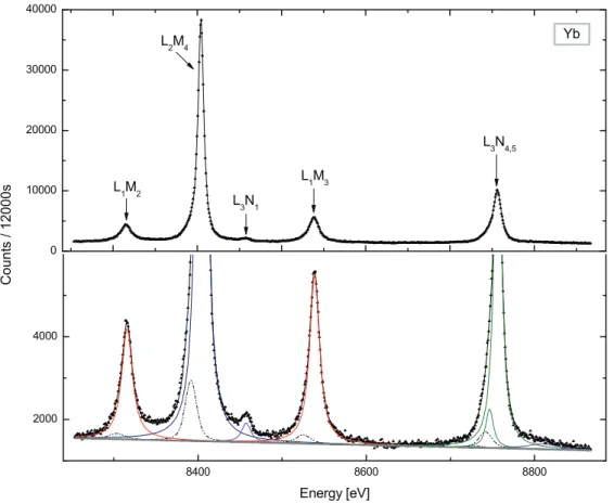
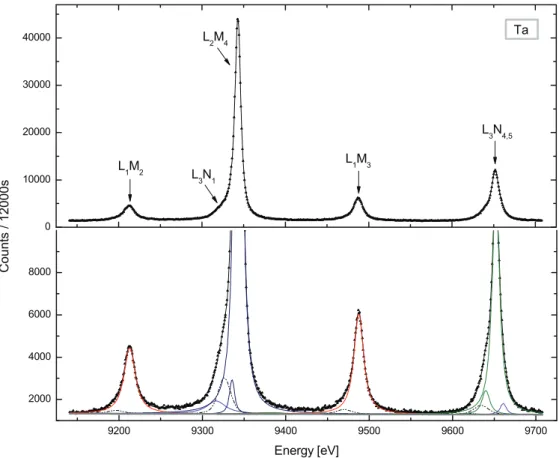
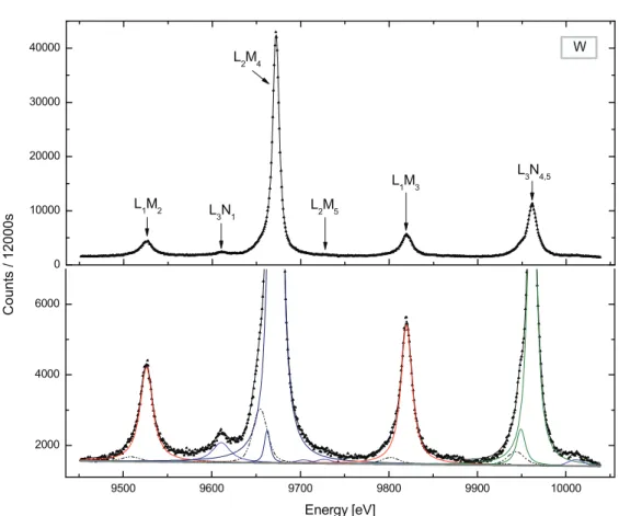
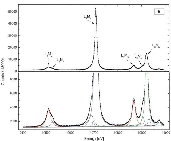
The fits of the L x-ray spectra measured with the von Hamos and DuMond spectrometers are presented in Figs. 7 to 12 and 13 to 18, respectively. It is interesting to see that in each spectrum the L1M2 and L1M3 transitions occur always below and above the strong L2M4

transition, whereas the relative positions of the L3 transitions change drastically with the

atomic number of the sample. For instance, the L3N1 line lies above the L2M4 line for 69Tm

(Fig. 7), between the L1M2 and L2M4 lines for 75Re (Fig. 12) and below the L1M2 line for 81Tl

(Fig. 14).

The L3N4,5 lines of 73Ta, 75Re, 77Ir, 81Tl and 83Bi evince asymmetries on their high energy

sides due to the presence of unresolved N spectator holes. Actually the energy shifts of satellites relative to the parent diagram lines increase with the principal quantum number of the transition electron and decrease with the principal quantum number of the spectator

(26)

M satellites of the strong L2M4 transitions were also observed in the spectra of 73Ta, 74W, 75Re

and 77Ir. Since L1L2M CK transitions are energetically forbidden for these elements, the weak

M satellites are probably due to M-shell shake processes following the photo-induced production of the 2p1/2 core vacancy.

0 10000 20000 30000 40000 L₃N₁ L₁M₂ _L 3N4 L₃N₅ L₂M₄ L₁M₃ L₂M₅ Tm 4000 6000 8000 Co unt s / 120 00s

(27)

In 69Tm, 71Lu, 73Ta, 74W, 75Re and 77Ir, small asymmetries were observed on the low energy

sides of the L2M4 transition. These asymmetries which result from the angular momentum

coupling between the L2 core vacancy and the partially filled outer shells was accounted for in

the fits by adding one or two additional Voigt functions. For Yb ([Xe]4f146s2), no asymmetry was observed since in the Yb crystal the two 6s electrons participate in the crystal bounding leaving the atom with a closed electronic shell configuration [24]. The same holds for Tl ([Hg]6p) and Bi ([Hg]6p3_{) which are generally monovalent and trivalent, respectively.}

For Ir (Fig. 13), the L1M2 and L3N1 transitions are strongly overlapping. Any attempt to let

free in the fitting procedure the energy and linewidth of the L3N1 line was found to be

unsuccessful so that these two parameters were kept fixed at the values taken respectively from Refs. [23] and [1].

Fig. 8: Same as Fig. 7 but for Yb. The line observed at about 8810 eV corresponds to the

M-satellite of the L3N4,5 transitions. 0 10000 20000 30000 40000 L₃N₁ L₁M₂ L₃N_4,5 L₂M₄ L₁M₃ Yb 8400 8600 8800 2000 4000 Cou nt s / 120 00s Energy [eV]

(28)

Fig. 9: Same as Fig. 7 but for Lu. The line observed at about 9114 eV corresponds to the M-satellite of the L3N4,5 transitions.

0 10000 20000 30000 L₃N₁ L₁M₂ L₃N_4,5 L₂M₄ L₁M₃ Lu 8600 8700 8800 8900 9000 9100 2000 4000 6000 8000 10000 Coun ts / 1200 0s Energy [eV]

(29)

Fig. 10: Same as Fig. 7 but for Ta. The lines observed at about 9381 eV and 9661 eV correspond respectively to the M-satellite of the L2M4 transitionand the N satellites of the L3N4,5 transitions. 0 10000 20000 30000 40000 L₃N₁ L₁M₂ L₃N_4,5 L₂M₄ L₁M₃ Ta 9200 9300 9400 9500 9600 9700 2000 4000 6000 8000 Cou nt s / 120 00s Energy [eV]

(30)

Fig. 11:Same as Fig. 7 but for W. The lines observed at about 9704 eV and 10011 eV correspond to the M-satellites of the L2M4 and L3N4,5 transitions, respectively.

0 10000 20000 30000 40000 L₃N₁ L₁M₂ L₃N_4,5 L₂M₄ L₁M₃ W L₂M₅ 9500 9600 9700 9800 9900 10000 2000 4000 6000 Co unt s / 120 00s Energy [eV]

(31)

Fig. 12: Same as Fig. 7 but for Re. The line observed at 10033 eV corresponds to the M-satellite of the L2M4 transition and those observed at 10285 eV and 10326 eV to the M and N satellites, respectively, of the L3N4,5 transitions.

0 10000 20000 30000 40000 50000 60000 L₃N₁ L₁M₂ L₃N₄ L₃N₅ L₂M₄ L₁M₃ Re 9800 9900 10000 10100 10200 10300 2000 4000 6000 Co unt s / 180 00s Energy [eV]

(32)

Fig. 13: Same as Fig. 7 but for Ir. The line observed at 10729 eV corresponds to the M-satellite of the L2M4 transition and those observed at 10929 eV and 10973 eV to the M and N satellites, respectively, of the L3N4,5 transitions.

0 10000 20000 30000 40000 50000 L₃N₁ L₁M₂ L₃N₄ L₃N₅ L₂M₄ L₁M₃ Ir 10400 10500 10600 10700 10800 10900 11000 2000 4000 6000 8000 Co unt s / 180 00s Energy [eV]

(33)

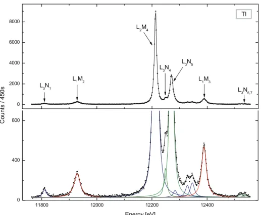
Fig. 14: High-resolution L x-ray spectrum of Tl measured with the Dumond spectrometer. The lines observed at 12329 eV and 12347 eV correspond to the M-satellites of the L3N4,5 transitions.

0 2000 4000 6000 8000 L₃N₁ L₁M₂ L₃N₄ L3N5 L₂M₄ L₁M₃ L₃N_6,7 Tl 11800 12000 12200 12400 0 400 800 C ount s / 450s Energy [eV]

Fig. 15: L1M2 and L1M3 x-ray lines of Tl measured with longer acquisition times than

the one used for the whole L spectrum represented in Fig. 14. In the analysis of the above partial spectra, only the parameters of the L1M2 and L1M3 transitions were let free, other fitting parameters (background, energies, widths and intensities of neighbouring lines) being kept fixed at the values obtained from the fit of the whole spectrum shown in Fig. 14 (for details, see text).

11800 11850 11900 11950 12000 12050 0 200 400 600 800 1000 Co un ts / 18 00 s Energy [eV] Tl L1M2 12300 12350 12400 12450 12500 0 400 800 1200 1600 Tl L1M3 C oun ts / 135 0 s Energy [eV]

(34)

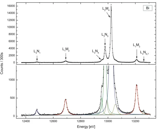
Fig. 16: Same as Fig. 14 but for Bi. The lines observed at 12990 eV and 13055 eV correspond respectively to the N and M satellites of the L3N4,5 transitions.

0 2000 4000 L₃N₁ L1M2 _L 3N4 L₁M₃ L₃N_6,7 12400 12600 12800 13000 13200 0 500 1000 C ount s / 300s Energy [eV] 800 1000 1200 1400 1600 1800 nts / 1 100 s Bi L1M2 800 1000 1200 1400 1600 1800 Bi L1M3 nts / 600 s

(35)

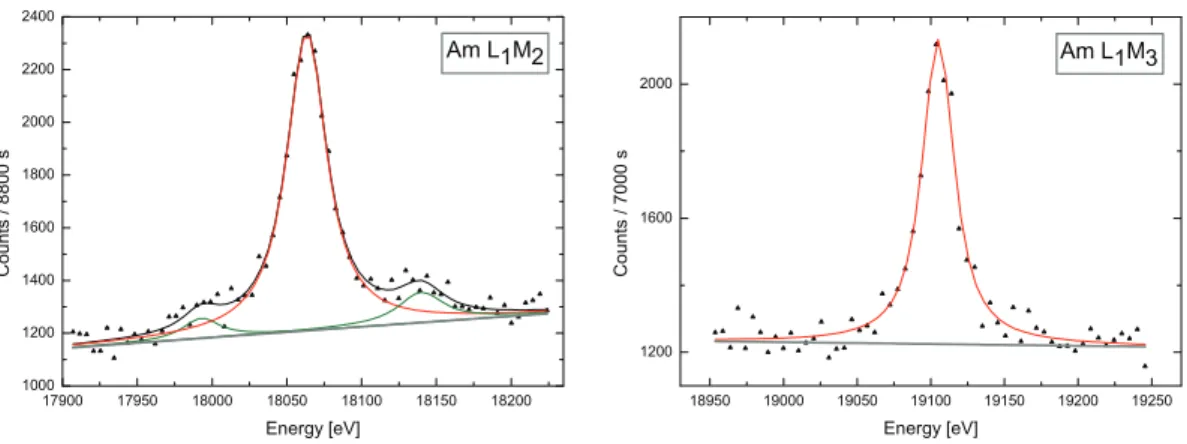
Fig. 18: Same as Fig. 15 but for ₉₅241Am. The line observed at about 18140 eV corresponds to the L3O1 transition and the one at about 17990 eV to the L1M3 transition of 93237Np which results from the α-decay of 24195Am. For this sample, due to the poor intensity of the fluorescence emission, we have renounced to measure the whole L x-ray spectrum.

17900 17950 18000 18050 18100 18150 18200 1000 1200 1400 1600 1800 2000 2200 2400 Cou nts / 8 800 s Energy [eV] Am L1M2 18950 19000 19050 19100 19150 19200 19250 1200 1600 2000 Am L1M3 Co unts / 70 00 s Energy [eV]

(36)

4.1 L

1

M

2,3

transition energies

The energies of the measured L1M2,3 transitions are given in Table 1 together with the

experimental and theoretical values reported recently by Deslattes et al. [23].

L1M2 transition energy [eV] L1M3 transition energy [eV]

Experiment Theory Experiment Theory Element Present Ref. [23] Ref. [23] Present Ref. [23] Ref. [23]

69Tm 8025.10(10/13)1 8025.8(1.5) 8026.1(2.6) 8233.75(11/13)1 8230.9(1.6) 8234.3(2.6) 70Yb 8313.36(42/43)1 8313.26(25) 8313.6(2.7) 8536.17(42/43)1 8536.79(43) 8536.8(2.8) 71Lu 8607.74(27/28)1 8606.54(44) 8606.3(2.7) 8846.73(28/29)1 8847.03(47) 8845.6(2.7) 73Ta 9212.82(30/31)1 9212.47(30) 9212.6(2.7) 9487.50(23/23)1 9487.62(32) 9487.1(2.8) 74W 9526.20(21/23)1 9525.23(54) 9526.0(2.8) 9819.95(12/13)1 9818.91(46) 9819.5(2.9) 75Re 9847.05(11/14)1 9846.35(58) 9846.8(2.8) 10160.29(19/20)1 10159.90(62) 10160.4(2.9) 77Ir 10510.42(3/11)1 10510.72(40) 10510.4(2.9) 10866.59(20/21)1 10866.54(42) 10867.5(3.0) 81Tl 11929.68(4/14)2 11930.78(51) 11931.0(3.0) 12389.40(4/9)2 12390.33(25/70)1 12390.55(55) 12390.6(3.2) 83Bi 12690.58(4/8)2 12691.40(77) 12690.9(3.1) 13209.57(4/9)2 13209.99(62) 13210.4(3.2) Am 241 95 18063.35(6/34)2 18062.96(78) 18065.7(3.5) 19104.98(6/40)2 19106.24(87) 19107.4(3.7)

1_{von Hamos spectrometer}2_{DuMond spectrometer}

Table 1: Energies of the L1M2 and L1M3 transitions. Present results are compared to theoretical and

(37)

contrast to that, about 35% of the experimental values listed in [23] are not consistent with our results, the biggest deviation being observed for the L1M3 transition of Tm (difference of 2.8

eV significantly bigger than the quoted error of 1.6 eV). It should be noted, however, that for the considered elements all experimental values reported in [23] were taken from the prior tabulation of Bearden [25]. Although these old Bearden’s data were re-adjusted in [23] to the new x-ray wavelength scale, they have to be regarded cautiously because several modern x-ray metrology measurements have shown that Bearden’s values deviate sometimes from the new results by several standard deviations, especially for weak x-ray lines. For instance, for the above-mentioned L1M3 transition of Tm, the Bearden’s value looks dubious since it is 3.4 eV

smaller than the corresponding theoretical prediction, whereas for the L1M2 transition of the

same element the difference with theory is only 0.3 eV.

For the measurements performed with the von Hamos spectrometer, the errors of present results originate mainly from the energy calibration procedure (see Table 1). In general, the energy uncertainty of transitions observed with the von Hamos spectrometer increases with the difference between the Bragg angles corresponding to the transition of interest and the transition employed as reference for the energy calibration. For instance, for Ir which was calibrated with the Kα1 transition of As (E = 10543.2674 ± 0.0081 eV [23]), the energy

calibration error of the L1M2 transition is only 0.03 eV because the Bragg angles

corresponding to the two transitions differ by less than 0.09 deg., whereas for the L1M3

transition, due to the bigger difference in the Bragg angles (0.8 deg.), the calibration error is approximately seven times bigger (0.20 eV). A further contribution to the relative big energy calibration errors affecting the measurements performed with the von Hamos spectrometer originates from the uncertainties on the energies of the transitions used as references. For the L1M3 transition of W which was calibrated with the Kα1 transition of Ge, the calibration error

is 0.11 eV although the two Bragg angles are similar (difference smaller than 0.2 deg.) because the energy of the Kα1 transition of Ge is only known with a poor precision (E = 9886.52 ±

0.11 eV [23]).

For the measurements performed with the DuMond spectrometer, quoted errors arise mainly from the fitting procedure, the uncertainty related to the energy calibration being small (0.04 to 0.06 eV). For Am, despite the long acquisition times used to measure the two transitions (about 170 h for the L1M2 transition and about 130 h for the L1M3), the errors given by the fits

were rather large (0.33 eV and 0.4 eV, respectively). The poor statistics of these measurements resulted mainly from the tiny dimensions of the employed sample. The effective surface of the latter was indeed only about 0.5 mm2 (75 mm2 for other samples) and its thickness 1.35 μm.

(38)

calculations seem to overestimate systematically our values by approximately 1.5%.

The energy difference between the M3 and M2 levels can also be derived from the

separation energy between the Kβ1 and Kβ3 x-ray lines. For tungsten, Kessler et al. [22] have

reported for these transitions energies of 67245.45 eV and 66952.40 eV. The precision of the measurements was 16 ppm. From these values an energy difference of 293.05 ± 1.52 eV is found, which is also in good agreement with the result of 293.75 ± 0.26 eV obtained from our measurements. Element Present MBPT [23] DF [26] 69Tm 208.65(18) 208.2 211.2 70Yb 222.81(61) 223.2 226.6 71Lu 238.99(40) 239.3 242.9 73Ta 274.68(39) 274.5 278.4 74W 293.75(26) 293.5 297.7 75Re 313.24(24) 313.6 318.0 77Ir 356.17(24) 357.1 362.2 81Tl 459.72(17) 459.6 466.0 83Bi 518.99(26) 519.5 526.6 Am 241 95 1041.63(52) 1041.7 1055.7

(39)

Finally, as mentioned in Chap. 2 the L1M3 transition of Tl was measured with both the

DuMond and von Hamos spectrometers. As shown in Table 1, the obtained energies are nearly consistent, a difference of 0.93 eV being observed which is 30% bigger than the error of 0.70 eV given for the von Hamos measurement. Note that this error is much bigger than the one corresponding to the measurement performed with the DuMond spectrometer because of the poor statistics of the von Hamos measurement. The latter had indeed to be performed in 2nd order of reflection, which resulted in a significant loss of the crystal reflectivity. In addition, for this relatively high energy (12.4 keV), the CCD efficiency was smaller than for other lighter elements.

4.2 L

1

M

2,3

transition widths

The L1M2 and L1M3 line widths obtained in the present work are presented in Table 3 and

Table 4, respectively. For comparison, the corresponding recommended values of Campbell and Papp [1] and theoretical predictions by Perkins [11] are listed, too. These data and other earlier experimental values are also represented graphically in Figs. 19 and 20. As shown, except for Bi, present L1M2 transition widths are systematically bigger (10%-20%) than the

values recommended by Campbell and Papp. For the L1M3 transition, the same trend is

observed but only for the elements Z ≤ 75.

1_{von Hamos spectrometer} 2_{DuMond spectrometer}

Experimental Theoretical

Z Present Campbell [1] Perkins [11] 69Tm 13.28(5/28)1 _{11.8(1.7) 16.10} 70Yb 15.00(5/25)1 _{12.3(1.8) 18.36} 71Lu 15.44(5/23)1 12.7(1.8) 19.29 73Ta 15.49(6/20)1 _{13.8(1.9) 21.49} 74W 16.23(7/29)1 _{14.4(1.9) 23.16} 75Re 18.43(7/26)1 15.1(2.0) 24.47 77Ir 19.61(7/33)1 _{16.8(2.5) 25.40} 81Tl 24.93(4/48)2 _{21.2(2.8) 27.03} 83Bi 23.01(6/23)2 _{23.0(2.9) 27.54} Am 241 95 30.47(11/1.16)2 - 31.70

Table 3: Natural line widths in eV of the L1M2 x-ray transition. Our experimental results are

compared to the recommended values of Campbell and Papp [1] and to theoretical predictions of Perkins [11]. The notation 13.28(5/28) eV means 13.28 ± 0.28 eV with an included contribution of ± 0.05 eV to the total error from the instrumental broadening uncertainty.

(40)

74W 14.06(8/19) 12.7(1.8) 27.74 75Re 15.48(9/19)1 13.6(1.9) 23.07 77Ir 15.25(12/24)1 _{15.9(2.4) 24.12} 81Tl 19.10(6/26)2 19.40(12/2.15)1 19.8(2.6) 24.23 83Bi 19.77(8/29)2 20.9(2.6) 24.86 Am 241 95 24.59(13/1.37)2 - 27.72

1_{von Hamos spectrometer}2_{DuMond spectrometer}

Table 4: Same as Table 1 but for the L1M3 x-ray transition.

From the two tables, it can be seen that for both spectrometers total errors arise mainly from the statistical errors given by the fits, the contribution of the errors on the instrumental broadening being negligibly small in most cases. The widths of the L1M3 transitions of Tl

measured with the DuMond and von Hamos spectrometers are in good agreement since they differ only by 0.3 eV, the error on the result obtained with the von Hamos spectrometer being seven times bigger (2.1 eV). As for the energy, this important error of 2.1 eV is due to the poor statistics of the measurement which was performed in second order of reflection.

Only three not too old data are available for comparison with the widths obtained in the present work. The first one concerns Ir for which a width of 15.1 ± 0.5 eV, in a fairly good agreement with our result of 15.25 ± 0.25 eV, is reported in [8] for the L1M3 transition. The

two other available data concern the L1M2 and L1M3 widths of W for which values of 15.0 ±

(41)

be again in quite satisfactory agreement with the widths of 22.6(3) eV and 18.6(3) eV, 27.6(7) eV and 23.6(3) eV, and 31.1(3) and 23.7(4) eV reported for Hg [13], Th [10] and U [9].

12 16 20 24 28 32 65 70 75 80 85 90 95

Fig. 19: Line width of the L1M2 transition versus atomic number. The

symbol ● corresponds to the results obtained in the present work, the solid line represents the recommended values of Campbell and Papp [1] and the dashed dotted line the calculations of Perkins [11]. Other plotted experimental data were taken from: □ Ref. [2], ∆ Ref. [3], ▲ Ref. [27], ○ Refs. [4, 7, 9, 10, 13].

L1 M2 li new id th [eV ] Z 65 70 75 80 85 90 95 10 12 14 16 18 20 22 24 26 28 30 L1 M3 li new idth [eV ] Z

Fig. 20: Line width of the L1M3 transition versus atomic number. The same

symbols as in Fig. 19 are used except for the experimental data represented by the symbol (○) which were taken from Refs. [7, 9, 10, 13, 6, 8].

(42)

fluorescence yields are small (less than 5.5% for the Z region studied in this work [28, 29]). As a consequence, the total M level widths are almost entirely due to non-radiative decay processes. According to Coster and Kronig [30], the probability of an Auger transition is proportional to the overlap between the wave functions of the initial and final states of both the transition electron and the ejected electron. Therefore, when they are energetically allowed, CK and especially super CK transitions (i.e. CK transitions involving three subshells of the same major shell) are highly probable and the level widths are governed mainly by these transitions. For the Z region concerned by this study, super CK transitions are energetically forbidden but there are several allowed CK transitions and the M2,3 level widths are mostly

due to them. In 74W for example, the calculations of Perkins [11] show that 77% of the M2

vacancies and 70% of the M3 vacancies are filled through CK transitions. Since the differences

between the electron binding energies in the subshells vary with the atomic number Z, certain CK transitions do exist only for elements belonging to specific Z regions of the periodic table [18]. The first element for which a given CK transition becomes energetically allowed or forbidden is called the onset or cut-off element for the considered CK transition.

Auger and Coster-Kronig transition probabilities for the M2,3 shells of elements with atomic

numbers 22 ≤ Z ≤ 90 were calculated by McGuire using a non relativistic Herman and Skillman potential and a semi-empirical estimation for the transition energies [31]. Chen et al. [28] reported relativistic calculations of non-radiative rates for the M1,2,3 subshells of 10

elements with 67 ≤ Z ≤ 95 based on a DHS potential. Using the results of Scofield’s DHS calculations for the radiative rates [32], they computed also the total M1,2,3 level widths. Their

(43)

4.3.2. Experimental M

2,3

atomic level widths

In the present work, the natural widths of the M2 and M3 subshells were determined from

the differences between the measured widths of the L1M2,3 transitions and the experimental

widths of the L1 subshell reported by Raboud et al. in [4]. Raboud’s results were preferred to

Campbell’s recommended values because the latter have errors 3-5 times bigger than the ones of Raboud. For the elements that were not measured in [4], linear interpolations between the two next neighbouring elements with Z below and above the atomic number of the element of interest were employed. For Tm, the L1 width was taken from the curve given by the authors

of [4] for the lanthanide region (see Fig. 21). In this region, a broadening of the 2s level was indeed observed. The latter was explained by a splitting effect [34] of the L1 subshell due to

an exchange interaction between the spin of the 2s level and the total spin of the unfilled 4f level. For Am, the L1 width was determined by a linear extrapolation of the values reported in

[4] for Bi and in [10] for Th and U.

Fig. 21: (taken from Ref. [4]): L1 level width versus atomic number Z. The solid line

represents the recommended values of Campbell and Papp [1], the dashed line results of independent-particle model calculations of Perkins et al. [11], and the dotted line predictions of the splitting model developed in Ref. [4] for the rare-earth elements. Experimental data from different sources are also presented, using the following symbols: (◊) x-ray absorption edge results from Refs. [35, 36], (∆) results derived from Coster-Kronig transition probabilities from Refs. [37, 38, 39], (□) XES results from Refs. [3, 40], (●) XES results for thorium and uranium from Refs. [9, 10], (○) XES results from Ref. [4].

(44)

Element L1 width [4] [eV] L1 width [1] [eV] M3 width [eV] Present M3 width [eV] Campbell [1] M3 width [eV] Perkins [11] 69Tm 5.45(32)1 _{4.9(1.5) 8.89(37) 7.1(9) 10.06} 70Yb 5.40(30) 5.2(1.5) 8.26(34) 6.7(9) 10.50 71Lu 5.65(33)2 _{5.4(1.5) 8.16(36) 6.0(8) 10.91} 73Ta 6.16(40)2 _{6.0(1.5) 6.78(42) 5.7(8) 10.19} 74W 6.41(43) 6.3(1.5) 7.65(47) 6.4(1.0) 10.12 75Re 6.94(50)2 _{6.7(1.5) 8.54(53) 6.9(1.1) 10.40} 77Ir 8.02(63)2 _{7.9(2.0) 7.23(67) 8.0(1.4) 10.98} 81Tl 11.28(68)2 11.1(2.0) 7.82(73) 8.7(1.7) 10.33 83Bi 12.50(45) 12.3(2.0) 7.27(54) 8.6(1.7) 10.82 95Am 16.63(30)2 _{- 7.96(1.40) - 11.49}

1_{From the curve calculated in [}₄_{] for the lanthanide region (see text)}2_{Interpolated value (see text)}

Table 5: M3 atomic level widths. Present results were deduced from the transition widths

quoted in Table 4 and the L1 level widths reported in [4] or interpolated from the latter. For comparison the L1 and M2 widths recommended by Campbell and Papp [1] and theoretical M2 widths of Perkins are also indicated.

Perkins probabilities [11] of all allowed M3 CK transitions for elements 65 ≤ Z ≤ 95 are

listed in Table 6. The broken curve in Fig. 22 corresponds to Perkins total M3 level widths

obtained by summing his computed radiative and non-radiative rates. The puzzling variations observed in this curve are fully accounted for by the changes in the probabilities of the CK transitions listed in Table 6. The drop around Z = 74 is due to the closing of the M3M4N3 and

(45)

available data, they extracted their recommended M3 level widths from the less old Cooper’s

data, i.e., those of 1944 [3].

Z Term 65 67 69 70 71 72 73 M3M4N2 1.39 10-2 1.28 10-2 - - - N3 6.68 10-2 _{6 10}-2 _{5.48 10}-2 _{5.24 10}-2 _{5.14 10}-2 _{5.22 10}-2 _{2.77 10}-2 N4 1.1 10-2 1.03 10-2 9.71 10-3 9.4 10-3 9.12 10-3 8.89 10-3 1.02 10-2 N5 9.79 10-3 _{9.38 10}-3 _{9.11 10}-3 _{8.94 10}-3 _{8.74 10}-3 _{8.61 10}-3 _{9.94 10}-3 N6,7 2.49 10-2 _{2.77 10}-2 _{3.04 10}-2 _{3.1 10}-2 _{3.13 10}-2 _{3.14 10}-2 _{3.63 10}-2 O1,2,3 1.02 10-3 9.1 10-3 8.27 10-3 7.82 10-3 7.84 10-3 7.91 10-3 9.36 10-3 M3M5N2 8.99 10-2 _{8.26 10}-2 _{7.8 10}-2 _{7.6 10}-2 _{7.49 10}-2 _{7.28 10}-2 -N3 1.51 10-1 _{1.36 10}-1 _{1.24 10}-1 _{1.18 10}-1 _{1.13 10}-1 _{1.09 10}-1 _{1.23 10}-1 N4 4.85 10-2 _{4.56 10}-2 _{4.34 10}-2 _{4.21 10}-2 _{4.08 10}-2 _{3.98 10}-2 _{4.57 10}-2 N5 7.19 10-2 _{6.64 10}-2 _{6.22 10}-2 _{6 10}-2 _{5.78 10}-2 _{5.61 10}-2 _{6.41 10}-2 N6,7 2.14 10-1 _{2.41 10}-1 _{2.68 10}-1 _{2.76 10}-1 _{2.79 10}-1 _{2.82 10}-1 _{3.29 10}-1 O1,2,3 4.08 10-2 _{3.62 10}-2 _{3.32 10}-2 _{3.15 10}-2 _{3.15 10}-2 _{3.18 10}-2 _{3.76 10}-2 Z Term 74 75 76 77 78 79 80 M3M4N2 - - - - N3 - - - - N4 1.04 10-2 1.03 10-2 1.02 10-2 9.93 10-3 9.8 10-3 1.04 10-2 1.15 10-2 M3M4N5 1.02 10-2 _{1.01 10}-2 _{1.01 10}-2 _{9.96 10}-3 _{9.88 10}-3 _{1.05 10}-2 _{1.15 10}-2 N6,7 3.79 10-2 _{3.78 10}-2 _{3.73 10}-2 _{3.71 10}-2 _{3.7 10}-2 _{3.88 10}-2 _{4.3 10}-2 O1,2,3 9.84 10-3 _{9.94 10}-3 _{1 10}-2 _{1.01 10}-2 _{1.03 10}-2 _{1.1 10}-2 _{1.25 10}-2 M3M5N2 - - - - N3 1.23 10-1 1.19 10-1 1.19 10-1 1.16 10-1 1.1 10-1 7.34 10-2 - N4 4.68 10-2 _{4.59 10}-2 _{4.51 10}-2 _{4.44 10}-2 _{4.38 10}-2 _{4.63 10}-2 _{5.08 10}-2 N5 6.53 10-2 _{6.37 10}-2 _{6.25 10}-2 _{6.12 10}-2 _{6.03 10}-2 _{6.34 10}-2 _{6.94 10}-2 N6,7 3.45 10-1 3.46 10-1 3.44 10-1 3.46 10-1 3.48 10-1 3.68 10-1 4.12 10-1 O1,2,3 3.97 10-2 _{4.03 10}-2 _{4.07 10}-2 _{4.07 10}-2 _{4.14 10}-2 _{4.45 10}-2 _{5.05 10}-2 O4,5 1.3 10-3 _{3.09 10}-3 _{4 10}-3 _{3.19 10}-3 _{6.4 10}-3 _{7.96 10}-3 _{9.84 10}-3 Z Term 81 82 83 84 85 86 87 M3M4N2 - - - - N3 - - - - N4 1.14 10-2 _{1.12 10}-2 _{1.09 10}-2 _{6.19 10}-3 _{- - -} N5 1.16 10-2 _{1.14 10}-2 _{1.15 10}-2 _{1.23 10}-2 _{1.19 10}-2 _{- -} N6,7 4.25 10-2 4.2 10-2 4.13 10-2 4.1 10-2 4.08 10-2 4.08 10-2 4.04 10-2 O1,2,3 1.27 10-2 _{1.29 10}-2 _{1.31 10}-2 _{1.34 10}-2 _{1.37 10}-2 _{1.43 10}-2 _{1.45 10}-2 O4,5 2.07 10-3 _{2.25 10}-3 _{2.41 10}-3 _{2.6 10}-3 _{2.79 10}-3 _{3 10}-3 _{3.15 10}-3 M3M5N2 - - - - N3 - - - - N4 5.02 10-2 _{4.93 10}-2 _{4.84 10}-2 _{4.84 10}-2 _{4.88 10}-2 _{4.97 10}-2 _{4.91 10}-2 N5 6.86 10-2 6.73 10-2 6.58 10-2 6.57 10-2 6.52 10-2 6.61 10-2 6.51 10-2 N6,7 4.1 10-1 _{4.09 10}-1 _{4.2 10}-1 _{4.1 10}-1 _{4.15 10}-1 _{4.2 10}-1 _{4.22 10}-1 O1,2,3 5.16 10-2 _{5.22 10}-2 _{5.28 10}-2 _{5.42 10}-2 _{5.56 10}-2 _{5.77 10}-2 _{5.86 10}-2 O4,5 1.09 10-2 _{1.17 10}-2 _{1.25 10}-2 _{1.33 10}-3 _{1.42 10}-2 _{1.51 10}-2 _{1.58 10}-2

(46)

M3M5N2 - - - - N3 - - - - N4 4.83 10-2 _{4.89 10}-2 _{4.4 10}-2 _{- - - -} N5 6.46 10-2 _{6.43 10}-2 _{6.36 10}-2 _{6.86 10}-2 _{6.54 10}-2 _{6.14 10}-2 _- N6,7 4.23 10-1 4.23 10-1 4.28 10-1 4.57 10-1 4.61 10-1 4.76 10-1 5.16 10-1 O1,2,3 5.94 10-2 _{6.05 10}-2 _{6.18 10}-2 _{6.7 10}-2 _{6.79 10}-2 _{7.13 10}-2 _{7.76 10}-2 O4,5 1.64 10-2 _{1.7 10}-2 _{1.76 10}-2 _{1.91 10}-2 _{1.94 10}-2 _{2.03 10}-2 _{2.21 10}-2

Table 6: Results of independent-particle model calculations of M3 CK transition rates for

elements with atomic numbers 65 ≤ Z ≤ 95 (taken from Ref. [11]).

3 4 5 6 7 8 9 10 11 12 13 50 60 70 80 90 100 M3 w idth [eV]

(47)

As shown in Fig. 22, in the Z region 69 ≤ Z ≤ 74, our results (red circles) exceed those of Salem and Lee [2], suggesting the possibility that the M3 level widths extracted from L1M3

line width measurements of Salem and Lee for lower atomic numbers (58 ≤ Z ≤ 68) might be also too low. Our data lie also systematically above those of Cooper [27]. However, as already reported in [42], Cooper’s data were probably overcorrected for the instrumental response. Furthermore, it can be seen in Fig. 22 that all experimental data lie significantly lower than the Perkins theoretical predictions [11]. Actually, Perkins himself mentioned that his computed CK transition rates may overestimate the true values by a factor up to two due to the small binding energies differences. This was also pointed out by Campbell and Papp [1, 41] who observed that Perkins calculations exceed largely the experimental widths for all levels dominated by CK decay, while they provide a fairly good approximation for other levels.

Z+1 rule Perkins [11] This work

M3M5N2 71 73 72 or 73 M3M4N3 72 74 72 or 73 M3M5N3 77 80 76 or 77 M3M4N4 83 85 82 or 83 M3M4N5 84 86 82 or 83 M3M5N4 89 91 - M3M5N5 91 95 -

Table 7: Cut-off atomic numbers of the M3M4N3,4,5 and M3M5N2,3,4,5 CK transitions.

Finally, it can be noted that our experimental values reveal the same puzzling variations as those observed in Perkins’s curve. However, they do not peak at the same atomic numbers indicating that the CK cut-off atomic numbers derived from the present measurements do not correspond to those predicted by Perkins’s calculations. Table 7 presents the cut-off atomic numbers deduced from our measurements, those predicted by Perkins and the Z+1 rule using the experimental binding energies tabulated by Storm and Israel [43]. The Z+1 rule appears to provide cut-off atomic numbers that are in better agreement with our experimental data than those deduced from Perkins calculations which yield systematically higher values. This may indicate that Perkins calculations overestimate the CK transition energies. Similar observations were done by Campbell for the M4M5N4,5 CK transitions. For the latter Perkins predicts indeed

the onset at Z = 49, while Martensson [44] measured a maximum rate for 44Ru and 45Rh and

the cut-off at Z=47. Similarly, for the L2L3M5 and L2L3M4 CK transitions, the onsets are