An adaptive control technology for flight safety in the presence of actuator anomalies and damage

An Adaptive Control Technology for Flight Safety

in the Presence of Actuator Anomalies and

MASSACHUSETTS INSi'fIJTE

Damage

OF TECHNOLOGY

by

MAR 2

2 2010

Megumi Matsutani

LIBRARIES

Submitted to the Department of Aeronautics and Astronautics

in partial fulfillment of the requirements for the degree of

Master of Science in Aeronautics and Astronautics Engineering

at the

_ARCHIVES

MASSACHUSETTS INSTITUTE OF TECHNOLOGY

Jan

2010

©

Massachusetts Institute of Technology 2010. All rights reserved.

A uthor ... ..

...----Department of Aeronautics and Astronautics

Jan 15, 2010

A

Certified by ... ... ...

Dr. Anuradha Annaswamy

Senior Research Scientist

Thesis Supervisor

A ccepted by ...

.

...

Prof. Eytan H. Modiano

Associate Professor of Aeronautics and Astronautics

An Adaptive Control Technology for Flight Safety in the

Presence of Actuator Anomalies and Damage

by

Megumi Matsutani

Submitted to the Department of Aeronautics and Astronautics on Jan 15, 2010, in partial fulfillment of the

requirements for the degree of

Master of Science in Aeronautics and Astronautics Engineering

Abstract

The challenge of achieving safe flight comes into sharp focus in the face of adverse conditions caused by faults, damage, or upsets. When these situations occur, the corresponding uncertainties directly affect the safe operation of the aircraft. A tech-nology that has the potential for enabling a safe flight under these adverse conditions is adaptive control. One of the main features of an adaptive control architecture is its ability to react to changing characteristics of the underlying aircraft dynamics. This thesis proposes the building blocks of an adaptable and reconfigurable control technology that ensures safe flight under adverse flight conditions. This technology enables the synthesis of such controllers as well as the systematic evaluation of their robustness characteristics.

The field of adaptive control is a mature theoretical discipline that has evolved over the past thirty years, embodying methodologies for controlling uncertain dynamic systems with parametric uncertainties [1, 2, 3, 4, 5, 6]. Through the efforts of various researchers over this period, systematic methods for the control of linear and nonlinear dynamic systems with parametric and dynamic uncertainties have been developed

[7, 8, 9, 10, 11, 12]. Stability and robustness properties of these systems in the presence of disturbances, time-varying parameters, unmodeled dynamics, time-delays, and various nonlinearities, have been outlined in the references [4]-[13] as well as in several journal and conference papers over the same period.

In this thesis, we consider the control of a transport aircraft model that resembles the Generic Transport Model [14]. While the vehicles' geometry and aerodynamic model are those of a C5 aircraft, every other aspect has been made to coincide with the GTM, e.g. anti wind-up logic, time-delay due to telemetry, baseline control struc-ture, low-pass and wash-out filters. We delineate the underlying nonlinear model of this aircraft, and introduce various damages, and failures into this model. An adaptive control architecture is proposed which combines a nominal controller that provides a satisfactory performance in the absence of adverse conditions, and an adaptive controller that is capable of accommodating various adverse conditions including ac-tuator saturation. The specific adverse conditions considered can be grouped into the

following three categories, (a) upsets, (b) damages, and (c) actuator failures. Specific cases in (a) include flight upsets in initial conditions of various states including an-gle of attack, cases in (b) include situations where structural failures cause changes in the location of the Center-of-Gravity (CG)[15], while cases in (c) include situa-tions where symmetric and asymmetric failures in control surfaces and engines occur. These failures include losses in control effectiveness, and locked-in-place control sur-face deflections.

The resilience of the adaptive controller to uncertainty is evaluated for safety using the control verification methodology proposed in [16]. This methodology enables the determination of ranges of uncertainty for which a prescribed set of closed-loop requirements are satisfied. This thesis studies several one-dimensional uncertainty analyzes for two flight maneuvers that focus on the longitudinal and lateral dynamics. As compared to the baseline controller, the adaptive controller enlarges the region of safe operation by a sizable margin in all but one of the cases considered.

Thesis Supervisor: Dr. Anuradha Annaswamy Title: Senior Research Scientist

Acknowledgments

Firstly, I would like to acknowledge my advisor Anuradha Annaswamy for educat-ing and guideducat-ing me to conduct great research, giveducat-ing me an opportunities to visit Technische Universitat Munchen in the spring of 2009 and NASA Langley Research Center in the summer of 2008 and 2009, and to have fruitful research interactions there. I would like to thank Luis G. Crespo at National Institute of Aerospace for many insightful discussions and for the support in conducting simulation studies. I would also like to thank to NASA IRAC project for supporting this work. Lastly, I want to thank my best friend Beni Yoshida for his support.

Contents

1 Introduction

1.1 Adaptive Flight Control . . . .

1.1.1 Adaptive Control . . . . 1.1.2 On-line Reallocation in the Presence of 1.2 Control Verification & Validation . . . .

1.2.1 Control Verification Methodology . . .

1.2.2 Generic Transport Model . . . .

1.3 Organization of this Thesis . . . .

2 The 2.1 2.2

Model of a Large Transport

Nonlinear Dynamic Model . . .

Adverse Conditions . . . . 2.2.1 Flight upsets: . . . . 2.2.2 CG movement: . . . . . 2.2.3 Actuator Failures: . . . . . . . . . . . . Actuator Failures . . . . . . . . . . . . . . . . Aircraft

3 Adaptive Control Architecture

3.1 Nominal Controller . . . .

3.1.1 Washout Filters and Low-pass Filters

3.1.2 LQR Controller with Integral Action

3.2 Saturation . . . .

3.3 Adaptive Controller... . . . . . . . . 7

4 Control Verification 4.1 Mathematical Framework . . . . 4.1.1 One-dimensional Case . . . . 4.2 Analysis Setup . . . . 4.2.1 Uncertain Parameters . . . . 4.2.2 Closed-loop Requirements . . . . 4.3 Flight Conditions (FC) . . . . 5 Results 5.1 One-dimensional Case . . . . . 5.2 Multi-dimensional Case . . . . .

6 Adaptive Control Design for the 6.1 Control Design . . . . 6.1.1 Baseline Controller . . . 6.1.2 Adaptive Controller . . . 6.2 Control Implementation . . . . 6.2.1 Reference Model . . . . 6.2.2 Adaptive Rate . . . . 6.3 Case Studies . . . . 6.3.1 Rudders Off . . . .

6.3.2 25% Left Wingtip Off . . 6.3.3 Aft CG Shift . . . .

6.4 Conclusions and Remarks . . . 7 Summary

Generic Transport Model

. . . . . . . .

List of Figures

3-1 Washout filters and low-pass filters . . . . 28

3-2 Control Architecture. . . . . 31

4-1 Relevant variables in the 1-dimensional parameter space. . . . . 37

4-2 Time simulation for the longitudinal flight condition. . . . . 40

4-3 Time simulation for lateral flight condition . . . . 40

5-1 Case A: g(Aa(0)) for the longitudinal FC. . . . . 43

5-2 Case B: g(Ax/cref) for the longitudinal FC. . . . . 44

5-3 Case C: g(Ay/bef) for the lateral FC . . . . 44

5-4 Case D: g(Aaii) for the lateral FC. . . . . 45

5-5 Case E: g(Ace) for the longitudinal FC. . . . . 46

5-6 Case F: g(Al2 ) for the lateral FC. . . . . 46

5-7 Case G: g(Atj) for the longitudinal FC. . . . . 47

5-8 Case H: g(ti) for the longitudinal FC. . . . . 47

5-9 Case I: g(r) for the longitudinal FC. . . . . 48

5-10 Time simulation for r = 0.74s. . . . . . . 49

5-11 Time simulation for multiple uncertainties. . . . . 50

6-1 Anti-wind up technique for e, and 6e. . . . . 56

6-2 Control Architecture. . . . . 60

6-3 Reference model. . . . . 63 9

6-4 States: Time simulation for Rudders Off. Line conventions are as follows: open-loop response with no damage (green, short-dashed line), open-loop with damage (red, solid line), closed-loop for the baseline controller with damage (cyan, dot-dashed line), closed-loop for the

adaptive controller with damage (blue long-dashed line). . . . . 65

6-5 States: Time simulation for 25% Left Wingtip Off. . . . . 66

6-6 States: Time simulation for CG shift. . . . . 67

6-7 Inputs: Time simulation for CG shift. . . . . 68

List of Tables

2.1 Aircraft states, actuators, and pilot inputs. . . . . 22

5.1 Cases analyzed . . . . 42

5.2 Numerical Values . . . . 42

Chapter 1

Introduction

1.1

Adaptive Flight Control

1.1.1

Adaptive Control

The field of adaptive control has addressed the problem of control of dynamic systems with parametric uncertainty [1]-[5],[17]. The simplest example is the control of a plant having the form

y = (W,(s, 0))u (1.1)

where W,(s) represents the aircraft dynamics linearized about a trim condition, 60 is the nominal value of the uncertain parameter 0, and u and y represent a vector of control inputs and measurable outputs. We will assume that 0 belongs to the set,

H(60, A) where A, the uncertainty radius, is proportional to the uncertainty we have

in the actual value of 0. H(0, A) may be due to uncertain aerodynamic coefficients, inaccurate atmospheric models, or actuator failures. The adaptive controller is given

by

where k(.) is a control parameter that is varied nonlinearly as a function of on-line measurements of the vehicle, J is a vector of command signals, and F is an adaptation gain. It is well known that the closed-loop system is guaranteed to be stable, and that the output tracks specified command signals arbitrarily closely under certain matching conditions. Yet another uncertainty that can be addressed is due to unmodeled dynamics whose effects may be due to atmospheric excitation, or flutter modes. If these effects are represented through the operator pA(s) , where A(s) has a bounded norm and p is a finite gain, the vehicle dynamics is now given by

y = (W,(s, 9) + pA(s))u. (1.3)

For every uncertainty model H, choice of an adaptation gain F, command signal 6 and performance metric, there exists a critical gain p*, that can be tolerated [4]. Bounds of p* have been derived for general uncertainties A(s).

1.1.2

On-line Reallocation in the Presence of Actuator

Fail-ures

The advantage of any adaptive control system is its ability to cope with unforeseen changes in the flight and environmental dynamics. Possible causes of such changes are actuator failure, vehicle geometry changes, and other disturbances. In [10], a direct-adaptive flight controller is proposed to enable reconfiguration in the presence of actuator failures, environmental disturbances, and modeling errors. The controller, developed using the K&A algorithm in [7] enables stable compensation in the presence of actuator failures via on-line reconfiguration and control allocation, while accom-modating for magnitude constraints on the control input. For the system in (1.3), an adaptive controller which incorporates reallocation over control surfaces is designed as

where G is a nonlinear reallocation algorithm which depends on Go, a constant re-allocation matrix, x is the state, and Xcmd is a command signal. Benefits of the

proposed adaptive controller were demonstrated using a linearized six-degree of free-dom simulation model of a large, four engine transport aircraft. It was observed that this algorithm provides improved performance compared to a standard adaptive algorithm.

1.2

Control Verification & Validation

1.2.1

Control Verification Methodology

The set of design requirements to be satisfied by the closed-loop system can be de-scribed by a collection of inequality constraints that depend on the uncertain pa-rameters and the design variables. In general, these requirements can be prescribed as

g(O, t, d, p, A) < 0 (1.5)

where d is the design variable. The projection of the constraint in (1.5) onto the 6-space partitions the uncertain 6-space into two regions, a region where the constraint is violated, called the Failure Domain F, and a region where the constraint is satisfied, called the Safe Domain. Depending on the requirement being cast by Equation (1.5), excursions into the Failure Domain could represent instability, poor handling qualities, or excessive control actuation.

The Parametric Safety Margin, whose evaluation requires the homothetic defor-mation of the set H(60, A), is the "distance between H(0, A) and the Failure Domain.

This deformation, which uses 00 as an anchor point while preserving the orientation and proportionality of H, is performed until the deformed set touches the boundary of the Failure Domain. The resulting deformed set is called the Maximal Set. The Parametric Safety Margin is a measure of the size of the Maximal Set. The larger the Parametric Safety Margin, the larger the smallest excursion from 00 required for

violating Equation (1.5), thus, the better the robustness.

When Equation (1.5) casts the stability and performance requirements on the closed-loop system, the Parametric Safety Margins unambiguously characterizes the resilience of the adaptive controller to uncertainty in 6. A methodology for robustness

analysis and robust design, based on Parametric Safety Margins, has been proposed in [18]. These robustness metrics can be used to evaluate the ability of control sys-tems to satisfy the closed-loop stability and performance requirements in the presence of uncertain physical parameters, control failures, and damage. Because this frame-work is applicable to nonlinear, possibly time-varying systems, where requirements that explicitly depend on time are present, these metrics are well suited for adaptive control.

The Parametric Safety Margins can also be used to systematically "robustify adap-tive controllers. By this we mean that we can search for a control architecture so that the set of free parameters maximize the robustness margins. This thesis does not tackle such a optimization problem though and applies the metrics only to the ro-bustness study of the adaptive control architecture to be designed in this thesis and to the evaluation of the improvement in flight safety attained by adaptation.

1.2.2

Generic Transport Model

The Generic Transport Model (GTM) is a dynamically scaled model of a transport aircraft for which NASA Langley has developed a high-fidelity simulink model. This simulation uses non-linear aerodynamic models extracted from wind tunnel data, and considers avionics, sensor dynamics, engine dynamics, atmospheric models, sensor noise and bias, telemetry effects, etc. This aircraft has ten controllable inputs and overall the open-loop plant has 278 states. As the actual vehicle itself, this model departs considerably from the Linear Time Invariant (LTI) system usually assumed for control design and therefore enables us to determine whether the improvements in stability, safety, and performance expected can be realized in practice. Using this vehicle, conducting a flight test is one of our plans to validate an adaptive control technology for flight safety. As well as the studies to be conducted in this thesis, this

strongly connects this mature theoretical discipline of adaptive control to the actual world, and leads to realization of actual applications of adaptive control on aerospace applications to achieve a safety flight.

1.3

Organization of this Thesis

In this thesis, we start with building the nonlinear dynamic model of C5, a large transport aircraft in Chapter 2. For this GTM-like model, we design an adaptive control architecture in Chapter 3. With the control verification metrics which is to be introduced in Chapter 4, we then evaluate the robustness of the adaptive system to uncertainties in Chapter 5. Based on the studies from the previous chapters, Chapter

6 presents developments of an adaptive controller for the GTM. Finally Section 7

Chapter

2

The Model of a Large Transport

Aircraft

In this chapter, we begin with a description of the nonlinear dynamic model of C5, a large transport aircraft whose aerodynamics data is available in [19]. We consider rigid body dynamics, aerodynamics, the effect of the control inputs and derive the

overall nonlinear flight model. We then discuss adverse conditions such as flight upsets, damages, and failures, and how to model them.

2.1

Nonlinear Dynamic Model

A typical dynamic model of an aircraft consists of the equations of motion,

aerody-namics, actuator dyaerody-namics, actuator saturation, and sensor dynamics. The standard conservation equations [20] describe the dynamics of u, v, and w, the body-fixed air-craft velocities; p, q, and r, the roll, pitch, and yaw rates; and the Euler angles

#,

0,

and V$. The aircraft's equations of motion are given by

X

it = g X- g sinO - qw + rv, (2.1)

Y

g

= + g cos 0 sin

#-ru

+ Pw, (2.2)

z

= izz [L + Izzpq - (Izz - Ivy)qr] +

jj

[N - Ixzqr - (Ivy - Ixx) pq] , (2.4)

ID ID

= [M - (Izz - Izz) pr - Iz (p2

- r2_)]

, (2.5)

r = [L + Izzpq - (Izz - Ivy) qr] + " [N - Ixzqr - (Iy - Ixx) pq] , (2.6)

ID ID

=p+ q sin0tan +rcos

#tan0,

(2.7)

9 = q cos # - r sin #, (2.8)

= (qsin# + r cos

#)

sec 9, (2.9)

In the above, ID = IxxIzz I2z; X, Y , and Z are the aerodynamic forces in body

axes at the nominal CG, and L, M, and N are the aerodynamic moments about the same point. The values of the gross aircraft weight W, the moments of inertia Izx, IYY, and Iz, as well as the product of inertia Ixz can be found in [19].

The following navigation equations determine x and y, the positions of the aircraft in the north and east directions respectively, as well as the altitude h:

S= u cos 0 cos 0

+v(-

cos

#

sin)

+

sin

#

sin0 cos@)+ (2.10) w(sin

#

sin4' + cos

#

sin 0 cos @),

= u cos 0 sin V + v(cos

#

cos4' + sin

#

sin 0 sin4@)+ (2.11)

w(- sin

#

cos @ + cos

#

sin 0 sin

4),

h = u sin0 -v sin# cos 0 - w cos

#

cos 0. (2.12)

It is often convenient to replace the body-fixed velocities with the true airspeed VT,

from the body-fixed velocities, neglecting wind and gust-induced effects, as VT = u2 + v2 + w 2, (2.13) tana = -, (2.14) U V sin/3 = VT(2.15)

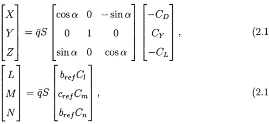
It is well known [21] that the aerodynamic forces and moments acting on the air-craft can be expressed in terms of the non-dimensional force and moment coefficients through multiplication by a denationalizing factor and, in the case of the forces, a transformation from wind to body axes. The forces and moments are therefore given

by

X

cos a 0 -sin a -CD

Y

qS

0

1

0

Cy

(2.16)

Z sina 0 cosa [-CLJ L bref CI

M

=

qS Cref

Cm

,

(2.17)

N bre5 Cn

where CL, CD, and Cy are the lift, drag, and side-force coefficients respectively while

C1, Cm, and Cn are the moment coefficients. The values of the the wingspan bre5, the mean aerodynamic chord cref, and the wing surface area S can be found in [19].

Table 2.1 shows the aircraft states, plant (i.e., inputs to the plant), control (i.e., outputs of the controller), and pilot inputs. The system state vector is given by

X = [VT a 0 p q r

p

6 x y h]T. (2.18)

The pilot inputs are ailerons, rudders, and elevators commands. Plant inputs are 4 engine throttles and the deflection of 6 control surfaces. As in the early version of the GTM the engines are not controllable. Therefore, the throttle values will be fixed at their trim values except for in Chapter 6.

Table 2.1: Aircraft states, actuators, and pilot inputs.

Variable Description Component of

Vt Velocity State (x) a Angle of Attack State (x)

#8 Side-slip Angle State (x) < Euler Angle State (x)

0 Euler Angle State (x)

1p Euler Angle State (x)

p Roll Rate State (x) q Pitch Rate State (x)

r Yaw Rate State (x)

t1 Left outboard Throttle Plant input

t2 Left Inboard Throttle Plant input t₃ Right Inboard Throttle Plant input t4 Right outboard Throttle Plant input

ei Left Elevator Plant input, Control output (u) e2 Right Elevator Plant input, Control output (u) a1 Left Aileron Plant input, Control output (u) a2 Right Aileron Plant input, Control output (u)

r1 Lower Rudder Plant input, Control output (u)

r2 Upper Rudder Plant input, Control output (u)

Je,cmd Virtual Elevator Pilot input (r)

6

a,cmd Virtual Aileron Pilot input (r)

6

The virtual inputs available to the pilot are the elevator, aileron, and rudder commands denoted as Aoe,cmd, A6a,cmd, and Ar,cmd. The aerodynamic force and moment coefficients are given by

CL = CLa + CL, 6e,

CD = CD, C + CD6 6e, (2.19)

C~~Cbref ± (Cyr _Cy.i5 bref YaYr

Cy =C,0 Y,~+p+ Cy'p ₂V + C, y1)kK - )v,( 2VT + CYs,,6a + Cy66,,

Ci= C1,30 + CpP + (C, -C )(r - b) + QCi,₆ a + C₆ ,6,, CM= Calph.a + (Cm + Cm)(q - 6) ₂ + Cm6 e, (2.20) VT Cn =Cn, flf~3'2 + Cnp fl VT + (Cn, - Cn4)(r -)r 2 VT + C, ~ 6a + Cn,6,,rr where 6_ ei + e₂ 2 6a = ai - a2 (2.21) 6 ri + r2 2

These set of equations prescribe the non-dimensional coefficients in Equations (2.16) and (2.17) as a a function of the state. In the context of Chapters 2-5, the control surface deflections are related to the control inputs by ui = ei, U2 = e2, U3 = ai,

U4 = a2, U5 = ri, and u6 - r2. Overall, the aircraft dynamics is given by the equations

above along with an aerodynamic model. The model to be used herein is prescribed subsequently.

We can compactly describe the overall nonlinear model as

X = F(X, AU) (2.22)

matrix.

For control purposes, the nonlinear plant is linearized about a trim point (Xo, UO) satisfying F(Xo, Uo) = 0. This leads to the linear time invariant system

=zAx + Bpu + g(xp, u) (2.23)

where

AP - F(X, U) B - OF(X, U) (2.24)

OX 'a

U

X0, UO X0, UO

and g(xp, u) is higher order terms.

2.2

Adverse Conditions

We now describe the three categories of upsets, damages, and failures that we shall introduce in the above model.

2.2.1

Flight upsets:

These adverse conditions result from large deviations in the initial conditions of the state from its trim value. If a system is stable, guarantees for a bounded performance are automatically obtained. Since in practical situations the closed-loop system is subject to unknown bounded disturbances, case for which only uniform ultimate boundedness can be proved, there are initial conditions for which the state may grow unbounded. Whether the actual responses are bounded and actually stay within limits of what is an acceptable remains to be demonstrated. In this paper, oZ(0) will be considered as an uncertain parameter. Since the baseline controller designed for the GTM does not enable lateral command following, flight upsets in

#(0)

were not studied.

2.2.2 CG movement:

A serious condition that needs to be addressed is structural damage. This causes,

among other things, a movement of the CG from its nominal position. Assuming that this movement only occurs in the xy plane, the changes to Equation (2.17) are given

by

AL = (Lcosa + Dsina)Ay

AM = -(Lcosa + Dsina)Ax (2.25)

AN = (Dcosa - Lsina)Ay

where Ax and Ay is the displacement from the nominal CG location to the post-failure one. The contribution of the tangential component of the acceleration can be accounted for by using the inertia tensor about the actual CG

I' = Izz + mAy2

I'/ =I +mAx 2 _(2.26)

I' = Izz + mAx2 + mAy2

In the studies that follow the contribution of the centripetal component of the accel-eration resulting from CG movement is ignored. The reader can refer to [15] for an explicit formulation of the equations of motion.

2.2.3

Actuator Failures:

We now consider adverse conditions that result from losses in control effectiveness and time delay.

As in reference [22], we model these failures by pre-multiplying the Bp matrix of the linearized model by the control effectiveness matrix A. That is, the Bp matrix in (2.23) is changed to BA where A is a matrix of dimension 6 x 6, which is equal to the identity matrix in the nominal case. Losses in control effectiveness are modeled

For example, if the right elevator fails by 50%, and the left aileron fails by 40%, A takes on the form

A = diag 1 0.5 0.6 1 1

1]-In general, the control effectiveness matrix takes the form

A = diag Aci Ae2 Aal Aa2 Ari Ar2 , (2.27)

where 0 < max{A} < 1.

In addition to these actuator failures we will also consider time delay in all six control inputs and control surface lock-ups. In the latter type, the uncertain pa-rameter is the duration of the lock-on-place failure. Note that from all uncertainties

Chapter 3

Adaptive Control Architecture

The control architecture proposed augments a nominal controller with an adaptive component. While the nominal controller is designed to meet the performance re-quirements under ideal operating conditions, the adaptive one copes with failures and uncertainties. The very same structure of the controller that Langley designed for the GTM will be used in the nominal controller. Details on such a structure are presented next.

3.1

Nominal Controller

The nominal controller has three main components, an array of low-pass and wash-out and filters, an LQR controller with integral action, and a hard-limiter to cope with control saturation. This limiter enforces an anti-integration windup logic based on the elevator deflection. This logic makes the system linear time varying. Each of these components is described in more detail next.

3.1.1

Washout Filters and Low-pass Filters

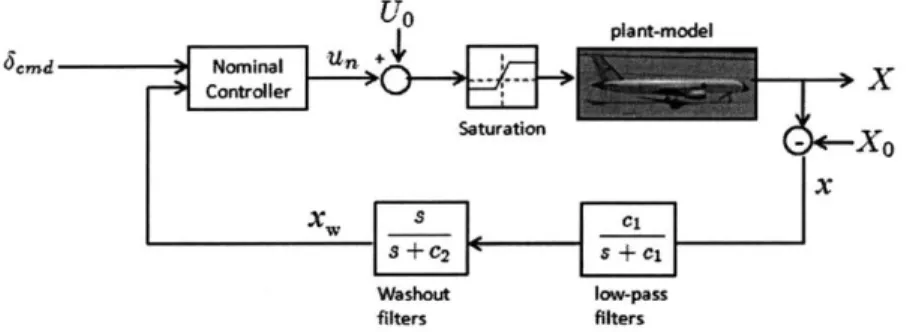
The GTM model has an array of low-pass and wash-out and filters to mitigate mea-surement noise and improve handling qualities. A block diagram of the system is shown in Figure 3-1. In particular, the states a, p, q, and r will be low-pass filtered

but only p, q, and r will be washed-out. These filters will be taken into account when designing the nominal controller.

I plant-model OcmdContre rX Saturation - _X x Washout low-pass filters filters

Figure 3-1: Washout filters and low-pass filters

3.1.2

LQR Controller with Integral Action

For control design purposes, we assume that the pitch, yaw and roll dynamics are weakly coupled. In order to closely follow a command in angle of attack, an integral state ec, is added

e. = f (a - acmd)dt (3.1)

where acmd = 106e,cmd. Note that elevator command does not affect elevator angle,

instead it generates integral error. The signal 6

e,cmd is one of the plant inputs in

r 1T

Jcmd = LJe,cmd 6a,cmd 6r,cmd . The augmented plant dynamics is therefore described

as

=P A

][x]

+

Bp

_{U +}

0acmd

[e H 0 eJ 0 -I

& A x B1 B2

Since the states in Equation (3.2) are accessible, an LQR controller is designed as

6en =- [Kea Keq K q

- -J (3.3)

6a,n

K[Kap

0

p

+

6a,cmd

6r'n

J

[0 K,,, [ J [r,cmdj

K,s5cmd

where the control gains K6 minimize the cost function

J = f (x' Rxxx + UT Ruuu)dt, (3.4)

and Rx, Ruu are weighting matrices. When only the baseline controller is used u =

Un = [6e,n, 6a,n, 6e,n] and that ei = e2 = 6e,n/2, ai = -a 2 = 6a,n/2 and r1 = r2 = 6r,n/2.

Equations (3.1)-(3.3) prescribe the closed-loop dynamics of an LTI approximation of the GTM for an LQR controller with integral action.

3.2

Saturation

To ensure that the control input does not exceed the saturation limits for the three control surfaces, the rectangular saturation function

R,(uj) = {m if ||UiI| < Ui,max, (3.5)

Ui,max sign(uj) if IIui|| > Ui,max,

is used. The control deficiency caused by saturation is given by

UA = U - R,(u). (3.6)

ea is also implemented. This logic is governed by the time-varying saturation function

Re(ea, 6e(t)) ec if

ea

> 0 or e, < eavailable,

(3.7)

eavailable if a < 0 and e >

eavailable-where eavailable is given by

(

Rs(6e) - (6e,trim + KseQOa + Keq q.) (.

eavailable = max

{0,

K3 .

(3.8)

The error deficiency caused by the saturation function in Equation (3.7) is defined as

eQA = ea - Re (ea, e(t)). (3.9)

By replacing u with R,(u,), and eQ with Re(ea, &c(t)) in Equation (3.2) we obtain

the LTV system

P

=

Ap

- BK

-BpKs,

x1

_Bp

_Kc

[eaj

L

H 0

J

[eaJ 0J

Am X Bi

+ a0cmd - [ u -BpKea ₁ eaA, (3.10)

-I 0 0

B2 R1 R2

which is the closed-loop system corresponding to the nominal controller. The bound-edness of this system can be established for all initial conditions inside a bounded set. This bounded set extends to the entire state-space when the open-loop plant is stable and there is no unmodeled dynamics (e.g., time-delay).

3.3

Adaptive Controller

Since the nominal controller in (3.3) has been designed for a plant-model under nomi-nal conditions, it may prove to be inadequate in the face of failures and uncertainties.

To mend for this we augment the controller in (3.3) with an adaptive component as

follows:

U = UO + Un + Ua = Uo + (K + 62)x + (Kr + 9r)r + f (3.11)

where 0,, Or, and

f

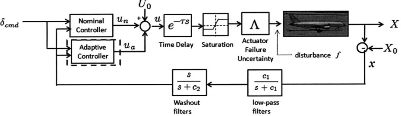
are adjusted to minimize the state error between the controlled plant-model and a reference model. The latter is chosen to generate the desired plant output for the commanded input. In the current problem, the reference model is given by the non-linear closed-loop system corresponding to the baseline controller for the case where there are no uncertainties. Besides, none of the saturation functions above are part of the reference model. Figure 3-2 shows the block diagram of this control architecture. Adaptive controllers for the GTM using a reference model that

.cmd

0 x

-X0

Washout low-pass filters filters

Figure 3-2: Control Architecture.

accounts for the time delay in telemetry have shown promise. Such controllers will be presented in Chapter 6.

Let xm be the state of the reference model. Defining the state error e as

e = x - xm

q0

we choose the adaptive laws for adjusting the adaptive parameters in (3.11) as Ox = -F1BTPeuxT -- aox Or = -F ₂BT Per - U2Or Tpe (3.13) f = -F 3BTPeU - U3Of A = -F 4diag(uA)B,'Pe -o4

where ATP + PAm = -Q,

Q

> 0, Pi is diagonal and positive definite for i = 1, ...4,

and eu = e - eA. The auxiliary error eA is defined as

eA = Ame - Ridiag(A)uA. (3.14)

Note that if the control does not saturate uA = 0, eA -+ 0 and eu -+ e. eA is the

error that occurs due to saturation, and by subtracting it out from e, we obtain eu which is the sum of the error due to uncertainties and the error due to e,,A. The o modifications prevent the drift of the adaptive parameters O0, 0r,

f

and A caused by

disturbances. The term

f

is an adaptive parameter aimed at counteracting constant disturbances.

It should be noted that the stability and boundedness of the closed-loop aug-mented system has been proved in [7, 11, 23] when physical saturation constraints are present. The stability analysis for the resetting-based anti-windup logic was also established and to be appeared elsewhere.

Chapter 4

Control Verification

This chapter introduces a framework for evaluating the degradation in closed-loop performance caused by increasingly larger values of uncertainty. This is attained by determining the largest hyper-rectangular set in the uncertain parameter space for which a set of closed-loop requirements are satisfied by all set members. A brief intro-duction to the mathematical framework required to perform this study is presented next. References [16] and [18] cover this material in more detail.

4.1

Mathematical Framework

The parameters which specify the closed-loop system are grouped into two categories: uncertain parameters, which are denoted by the vector p, and the control design parameters, which are denoted by the vector d. While the plant model depends on

p (e.g., aerodynamic coefficients, initial conditions, time delay, actuator failures), the

controller depends on d (e.g., control gains). The Nominal Parameter value, denoted as p, is the value that p assumes when there is no failure/uncertainty. The value of d on the other hand is assumed to be available and will remain fixed.

Stability and performance requirements for the closed-loop system will be pre-scribed by the set of constraint functions, g(p, d) < 0. This vector inequality, as all

others that follow, hold component wise. For a fixed d, the larger the region in p-space where g < 0, the more robust the controller. The Failure Domain corresponding to

the controller with parameters d is given byl

dim(g)

.F(d)=

U

Fj(d). (4.1)

j=1

Fi(d) = {p : gj (p, d) 0}, (4.2) While Equation (4.2) describes the failure domain corresponding to the jth require-ment, Equation (4.1) describes the failure domain for all requirements. The

Non-Failure Domain is the complement set of the failure domain and will be denoted2 as

C(F). The names "failure domain" and "non-failure domain" are used because in

the failure domain at least one constraint is violated while, in the non-failure domain, all constraints are satisfied.

Let Q be a set in p-space, called the Reference Set, whose geometric center is the nominal parameter . The geometry of Q will be prescribed according to the relative levels of uncertainty in p. One possible choice for the reference set is the

hyper-rectangle

7Z(,n)=f{p:zp-n p .ii+n}. (4.3) where n > 0 is the vector of half-lengths. One of the tasks of interest is to assign a measure of robustness to a controller based on measuring how much the reference set can be deformed before intersecting the failure domain. The Homothetic Deformation of Q with respect to the nominal parameter point - by a factor of a > 0, is the set

7-(Q, a) =

{p

+ a(p -

)

: p c Q}. The factor of this deformation, a, is called

the Similitude Ratio. While expansions are accomplished when a > 1, contractions result when 0 < a < 1. Hereafter, deformations must be interpreted as homothetic expansions or contractions.

In what follows we assume that the controller d satisfies the requirements for the nominal plant, i.e., g(p, d) < 0. Intuitively, one imagines that a homothet of the reference set is being deformed until its boundary touches the failure domain. Any

'Throughout this thesis, super-indices are used to denote a particular vector or set while sub-indices refer to vector components, e.g., pji is the ith component of the vector p3.

point where the deforming set touches the failure domain is a Critical Parameter

Value (CPV). The CPV, which will be denoted as p, might not be unique. The

deformed set is called the Maximal Set (MS) and will be denoted as M. The MS is the largest homothet of Q that fits within C(F). The Critical Similitude Ratio

(CSR), denoted as d, is the similitude ratio of that deformation. While the CSR is a non-dimensional number, the Parametric Safety Margin (PSM), denoted as p and defined later, is its dimensional equivalent. Both the CSR and the PSM quantify the size of the MS. Details on the implementation of these ideas are presented next.

The CPV corresponding to the deformation of Q = Z(p, n) for the jth requirement

is given by

=arg min {Op - -1| : gj(p, d) > 0, Ap > b}, (4.4)

P

where |llxH = supi{|xil/ni} is the n-scaled infinity norm. The last constraint in Equation (4.4) is used to exclude regions of the parameter space where plants are infeasible and uncertainty levels are unrealistic. The overall CPV is

p = pk, (4.5)

where

k =

arg min

{l|p

-

P||}

.

(4.6)

1 jidim(g)

The critical requirement, which is the one preventing a larger deformation, is gk < 0.

Once the CPV has been found, the MS is uniquely determined by

M(d) = R(p, &n). (4.7)

where & = ||p - -|| . The Rectangular PSM is defined as

p=&|n||,

(4.8)

The last two equations, which apply to the overall CPV, can be extended to individual

individual PSM.

Because the CSR and the PSM measure the size of the MS, their values are pro-portional to the degree of robustness of the controller associated with d to uncertainty in p. The CSR is non-dimensional, but depends on both the shape and the size of the reference set. The PSM has the same units as the uncertain parameters, and depends on the shape, but not the size, of the reference set. If the PSM is zero, the controller's robustness is practically nil since there are infinitely small perturbations of P leading to the violation of at least one of the requirements. If the PSM is posi-tive, the requirements are satisfied for parameter points in the vicinity of the nominal

parameter point. The larger the PSM, the larger the (-shaped vicinity.

4.1.1

One-dimensional Case

In the case where dim{p} = 1, the expressions for the CPVs, the PSM, and the MS

are given by S=arg min {jp - pl :g(p, d) > 0, Ap 2 b}, (4.9) P p =pk, (4.10) P p 1 (4.11) M(d) = (P - p, f + p), (4.12) where

k = arg min

{ip

-p}. (4.13)

1<j<;dim(g)

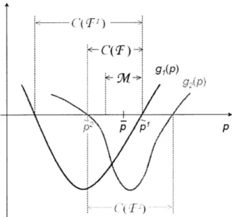
Figure 4-1 shows an sketch with relevant variables and sets. Note that the non-failure domain is given by the intersection of the individual non-failure domains. Besides, the overall CPV is the parameter value closest to the nominal point where at least one component of g is equal to zero. From the figure we see that l -

p

< p2 So P =

P

and k = 1. By construction, all the points within the MS, which is centered

about the nominal parameter point, satisfy the closed-loop requirements.

individu-Figure 4-1: Relevant variables in the 1-dimensional parameter space.

ally are unable to capture the effect of the dependencies among uncertain parameters. When such dependencies are important, the collection of PSMs that result from per-forming dim(p) one-dimensional deformations can misrepresent the actual system's robustness. For instance, if p1 is the PSM corresponding to a one-dimensional defor-mation in pi, p2 _{is the PSM corresponding to a one-dimensional deformation in}

P2,

and p3 is the PSM corresponding to a two-dimensional deformation in [Pi,P2]; it is

possible to have p3

_<

_{min{pI, p}2_{}. In such a case there is a combination of uncertain}

parameters much closer to

p

that will be missed by both one-dimensional searches.

4.2

Analysis Setup

4.2.1

Uncertain Parameters

We will consider the following set of uncertain parameters

-where the first 6 components, can be categorized as actuator uncertainties or fail-ures, the next two account for structural failures and last one for a flight upset. In particular,

Aeie =

Aei,

Ae2

Aaii

LAal,

Aa2 (4.15)

Arud [Arl, Ar2(

Athr [At I, At2, A3, At4

are the control effectiveness of elevators, ailerons, rudders, and engine throttle; r is a time delay in all input channels, and t is the duration of a control surface lock-up. The terms

A.

and AY are components of the position vector in the xy-body frame of the post-failure CG location with respect to a reference point. The last component, which models a flight upset, is the initial condition in angle of attack. The nominal parameter values corresponding to the set of parameters in Equation (4.14) is [1, 1, 1, 1, 0, 0, 0, 0, 01.

4.2.2

Closed-loop Requirements

The following stability and performance requirements will be considered

go = max{ [Utrim - Umax, Umin - Utrim]}, (4.16)

gi= max - 2.5, (4.17)

[ 9

93 = T(p, d) - c2 71(p, dbase), (4.19)

17 = wiIl a - acmdll2 + w211p - PcmdII2 I w317 -

TcmdiI2-The first requirement, go < 0, is used to determine if the vehicle has enough control authority to trim, i.e. if it satisfies Umin < Utrim < Umax. Note that this requirement

is independent of d and may indicate instability. gi < 0 is a structural requirement enforced by preventing the loading factor from exceeding the upper limit of 2.5. The requirement 92 < 0, where 0 < ci < 1, ke, > 0 and k,3 > 0, enforces stability and

satisfactory steady state performance. The last requirement, 93 < 0, for c2 > 1,

W1 > 0, w2 > 0 and w3 > 0, is used to measure satisfactory transient performance.

This requirement prevents the cumulative error from exceeding a prescribed upper limit. Such a limit is c2 times larger than the cumulative error incurred by the baseline

controller under nominal flying conditions.

In practice, control requirements are prescribed in advance before the control de-sign process even starts. When such requirements are only described qualitatively several g implementations are possible. This creates the additional challenge of con-structing functional forms that capture well the intent of the requirement while having a minimal amount of conservatism. This thesis does not tackle such a challenge and assumes that the g above is given.

4.3

Flight Conditions (FC)

The closed-loop response depends on p and d as well as on the intended flight ma-neuver

f.

This implies that g(p, d,

f).

Two flight conditions, namely

fr,,

and flat, will be considered in the analyzes that follow. In the former one, which mostly af-fects the longitudinal dynamics, a step input in 6

e,cmd is commanded. In the second

one, which affects both the longitudinal and lateral dynamics, the vehicle also starts from level flight and a set of commands in 6

a,cmd and 6r,cmd makes the vehicle turn.

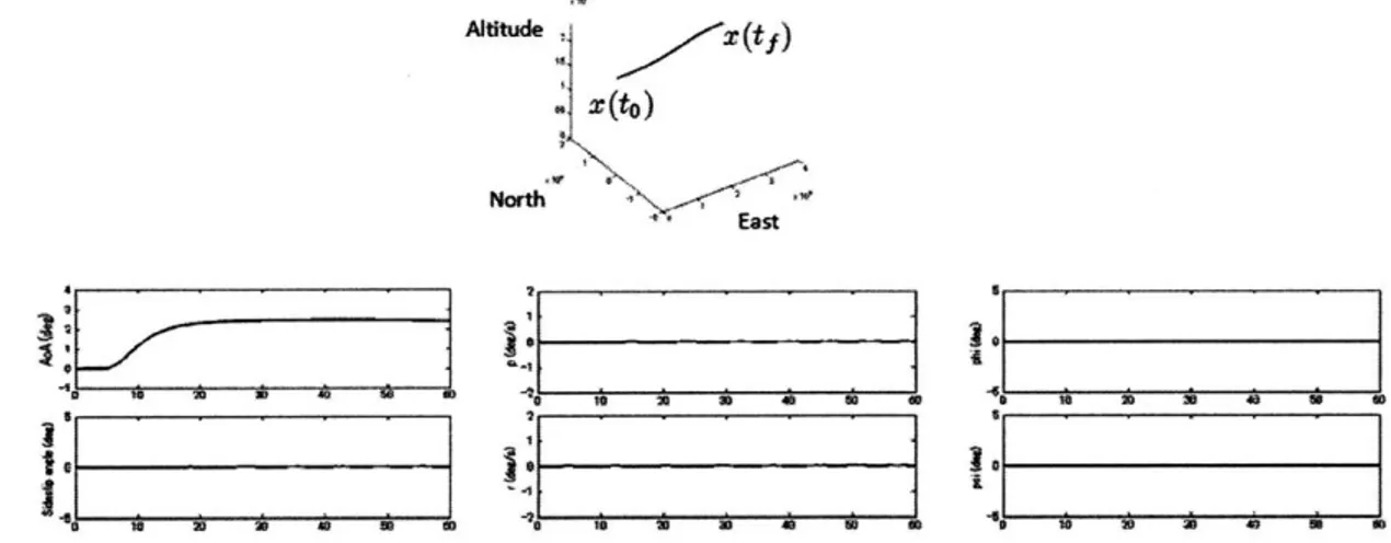
Figures 4-2 and 4-3 show the vehicle's trajectory as well as relevant states for both flight conditions when there is no uncertainty/failure. The p command for flat is a

sequence of two step inputs (only one is shown) where the second one is commanded so that it cancels the first one after a suitable time.

dtude _2E(tf) . (to) East 1 10 * 10 10 10 40 10 01 lit Figure 4-2: Time ~ J 10 10 10 40 01

I

0 -10 10 10 10 4 U 10 I 10 - 10 U

ii

simulation for the longitudina

UitUdo jz(to) North 20~ 10 10 10 10 I 4

~

:1

U 10 10 10 U 01 4* 10 10 10 10 U 10 1 flight condition. 10.

2

a U1 ~1__ ____ ____ ____ ___ ___ ____ ____ ___ ___ tooI 10 ~ 4 ~ 0 ~ 1 ~ ~ O ~ -1 A0 1 A0 0 1 it 10so10 a0

Chapter 5

Results

In this chapter, we evaluate the baseline controller in Equation (3.10) and the adaptive controller in Equations (3.11) - (3.14) according to the control verification setting of Chapter 4. The aerodynamic model used can be found in [19]. The numerical value of other variables are shown in Table 5.2.

5.1

One-dimensional Case

In Case A we consider a flight upset in the angle of attack, Aa(0) about atrim =

2.20(deg) for the longitudinal flight condition. The dependency of g on Aa(0) for both controllers is illustrated in Figure 5-1. The dashed lines and the solid lines represent results from the baseline and adaptive controllers respectively. A comparison of these curves shows that the non-failure region of the adaptive controller is larger by virtue of the structural and tracking performance requirements. The same line convention used in this figure applies to those that follow.

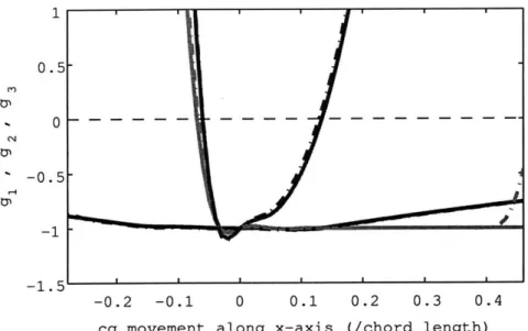
In Case B we consider the movement of the CG in the x-direction for the longi-tudinal flight condition. Recall that a positive value of the CG movement denotes a forward movement. Figure 5-2 illustrates the dependency of g on the CG location for both controllers. Note that the system loses stability when the CG moves backward, while the tracking performance degrades the faster when the CG moves forward. The baseline controller has a PSM of 0.175 while the adaptive one attains a PSM of 0.197.

Table 5.1: Cases analyzed

Case Failure/Uncertainty

Case A Flight upset in angle of attack [Aa(O) fA0o]

Case B CG movement along x-axis [A,

fron]

Case C CG movement along y-axis [Ay fiat]

Case D Symmetric Aileron failure [Aaii fiat]

Case E Symmetric Elevator failure [Acie fion] Case F Asymmetric Aileron failure [Aai flat]

Case G Asymmetric Throttle failure [Au fion]

Case H Elevator lock-in-place failure [tl fion]

Case I Time delay in all control inputs [r fion]

Table 5.2: Numerical Values

Variable Value Velocity at trim 614(ft/sec) Angle of Attack at trim 2.2(deg) Height at trim 20000(ft) Kse -0.4420 K6e -0.9105 K₆ -0.7906 Koa -0.1000 -0.3000 1 diag([1, 1, 100, 100, 100, 100]) x 200 F2 diag([1, 1, 100, 100, 100, 100]) x 100 13 diag([1, 1, 100, 100, 100, 100]) x 50 F4 diag([1, 1, 1, 1, 1, 1]) x 100 Q diag([1, 1, 1, 1, 1])

0.5-- g adaptive I, - g2 adaptive -- g3 adaptive 0 ---- --- ~- ~~~~---U-- - baseline - baseline -- , - - g 3 baseline ---- 0 line -1.5 1 2 3 4

initial condition alpha(O) (deg)

Figure 5-1: Case A: g(Aa(O)) for the longitudinal FC.

In Case C we consider the movement of the CG in the y-direction for the lateral flight condition. In this setting a positive CG movement denotes a movement to the right. Figure 5-3 illustrates the dependency of g on the CG location for both controllers. The curves are asymmetric with respect to the nominal parameter value, since the flight condition is itself asymmetric. As before, the adaptive controller attains a larger PSM. The baseline controller has a PSM of 0.0029 while the adaptive one attains a PSM of 0.0069.

In Case D, we consider a symmetric failure in both ailerons, where Aaii = Aai = Aa2,

for the lateral flight condition. Figure 5-4 illustrates the dependency of g on Aati for

both controllers. As before, the adaptive controller attains a larger PSM. While the PSM for the baseline is 6.6%, the PSM for the adaptive is 10%. In both cases, the tracking performance is the critical requirement.

In Case E we consider a symmetric failure in both elevators, where Aee = Ae, = Ae2, for the longitudinal flight condition. Figure 5-5 illustrates the dependency of g

on Aee for both controllers. While the PSM for the baseline is 33%, the PSM for the adaptive is 42%. In both cases, the tracking performance is the critical requirement.

-0.2 -0.1 0 0.1 0.2 0.3 0.4

cg movement along x-axis (/chord length)

Figure 5-2: Case B: g(Ax/cef) for the longitudinal FC.

-0.01 -0.005 0 0.005 0.01

cg movement along y-axis (/wing span)

Figure 5-3: Case C: g(Ay/bref) for the lateral FC.

-0.

As before, the adaptive controller has better robustness characteristics.

Unlike Case C, Case F considers an asymmetric aileron failure where A, is un-certain and A,2 = 1. Figure 5-6 illustrates the dependency of g on A, for both

controllers. While the PSM for the baseline is 14%, the PSM for the adaptive is 20%. Consistently, the tracking performance requirement remains being critical. We note however that the PSM corresponding to the stability requirement for the adaptive controller becomes smaller.

2 1.5 0.5 % % 0--- --- ---- --- --0.5' -1 -1.5 -2 0.4 0.5 0.6 0.7 0.8 0.9 1

control effectiveness in ailerons

Figure 5-4: Case D: g(Aai) for the lateral FC.

In Case G we consider a failure in the left outboard engine At, for the longitudinal flight condition. Figure 5-7 illustrates the dependency of g on At, for both controllers. While the PSM for the baseline is 1.7%, the PSM for the adaptive is 2.9%. As before, the tracking performance is the critical requirement. We note that the margins obtained in this case are considerably smaller than those found in the other cases. The non-failure domains are small since the throttle inputs are not controlled and remain fixed at their trim values. Results similar to those in Figure 5-7 were observed when the lateral flight condition was used.

A lock-in-place failure in the left elevator is considered in Case H. This is simulated by keeping this control input at a constant value for a period of tj seconds. The larger

0-0. 2

-- 0.4

0.4 0.5 0.6 0.7 0.8 0.9

control effectiveness in elevators

Figure 5-5: Case E: g(Aee) for the longitudinal FC.

-'-0. 5

-1.51 -2

-0.2 0.4 0.6 0.8

control effectiveness in left aileron

-2 '

0.2 0.4 0.6 0.8

left outboard throttle effectiveness

Figure 5-7: Case G: g(Ati) for the longitudinal FC.

10 5 0 -5 -10 0 0.5 1 1.5 2 2.5 3

lock-in-place duration time (sec)

the tj the more severe the failure. Figure 5-8 illustrates the dependency of g on the lock-in time. Substantial differences in the functional dependencies are apparent. It can be seen that the PSM for the baseline is 1.1 while the PSM for the adaptive is 2.1. We also note that while the tracking performance is critical for the baseline controller, the stability requirement is critical for the adaptive one.

Case I considers the case when there is a time delay r in all three control inputs. Figure 5-9 illustrates the dependency of g on this uncertain parameter for the longi-tudinal flight condition. In contrast to all other cases, the non-failure domain of the adaptive controller is smaller than that of the baseline. Hence, the nominal controller is more robust to uncertainty in the time delay than the adaptive one. One may infer that this is the price of attaining improved system performance through aggressive actuation. We however note that this observation may not hold when multiple uncer-tainties occur simultaneously. Figure 5-10 shows time responses for both controllers when r = 0.74s. This point belongs to the non-failure domain of the baseline con-troller and to the failure domain of the adaptive one.

0.5-0 - - - - - - - - - - - - - - - - - -- I -0.5--1 -1.5 0 0.2 0.4 0.6 0.8

time delay (sec)

Figure 5-9: Case I: g(r) for the longitudinal FC.

10 20 30 40 50 60 0 10 20 30 40 50 60

0 10 20 30 40 50 60 0 10 20 30

Time (sec) Time (sec)

Figure 5-10: Time simulation for r = 0.74s.

Table 5.3: Summary for

20 10 0 --10 0

20

the results of all cases

Case ap - 1) x 100% Critical Requirement

A +4.01 % 91,93 B +11.4 % 92, 93 C +133 % 92, 93 D +63.6 % 93 E +27.3% 93 F +46.7 % 93 G +70.6 % 93 H +88.9 % 92, 93 I -13.9 % 92, 93

attained by the adaptive controller and the critical requirement. In all but one of the cases considered, the adaptive controller attains better robustness by a sizable margin.

5.2

Multi-dimensional Case

In all the cases above only a single uncertain parameter has been considered. In this setting, the effect of the dependencies among parameters can not be captured. The same analysis can be conducted for a multi-dimensional vector p. In such a case, multiple failures and uncertainties occur simultaneously and the correlation among them may play a significant role. Studies of this type will be presented elsewhere. However, Figure 5-11 presents a time simulation of the controlled response for a

dimensional parameter realization when 2 pitch doublets are commanded. Therein, we assume losses in control effectiveness of 30% for the elevators, 10% for the ailerons, and 10% for the rudders. Besides, the CG has been moved to the left by 0.004/cref, and a flight upset in the angle of attack of 0.2 degrees is assumed. It is apparent that the adaptive controller achieves good tracking performance while the nominal controller can not recover and makes the system unstable.

20 40 60 0 20 40 60 V %* V ) 20 40 60 Time (sec) 20 40 60 20 40 60 20 40 60 Time (sec)

Figure 5-11: Time simulation for multiple uncertainties.

-5 -10 50 -0 50 50 50 50 -100