Water temperature drives phytoplankton blooms in coastal waters

HAL Id: hal-02358391

https://hal.archives-ouvertes.fr/hal-02358391

Submitted on 11 Nov 2019

HAL is a multi-disciplinary open access archive for the deposit and dissemination of sci-entific research documents, whether they are pub-lished or not. The documents may come from teaching and research institutions in France or abroad, or from public or private research centers.

L’archive ouverte pluridisciplinaire HAL, est destinée au dépôt et à la diffusion de documents scientifiques de niveau recherche, publiés ou non, émanant des établissements d’enseignement et de recherche français ou étrangers, des laboratoires publics ou privés.

coastal waters

Thomas Trombettaid, Francesca Vidussi, Sébastien Mas, David Parin,

Monique Simierid, Behzad Mostajir

To cite this version:

Thomas Trombettaid, Francesca Vidussi, Sébastien Mas, David Parin, Monique Simierid, et al.. Water temperature drives phytoplankton blooms in coastal waters. PLoS ONE, Public Library of Science, 2019, �10.1371/journal.pone.0214933�. �hal-02358391�

Water temperature drives phytoplankton

blooms in coastal waters

Thomas TrombettaID1*, Francesca Vidussi1, Se´bastien Mas2, David Parin2, Monique SimierID3, Behzad Mostajir1

1 MARBEC (Marine Biodiversity, Exploitation and Conservation), Centre National de la Recherche

Scientifique, Universite´ de Montpellier, Institut Franc¸ais de Recherche pour l’Exploitation de la Mer, Institut de Recherche pour le De´ veloppement, Montpellier, France, 2 MEDIMEER (Mediterranean Platform for Marine Ecosystems Experimental Research), Observatoire de Recherche Me´diterrane´ en de l’Environnement, Centre National de la Recherche Scientifique, Universite´ de Montpellier, Institut de Recherche pour le De´veloppement, Institut National de Recherche en Sciences et Technologies pour l’Environnement et l’Agriculture, Sète, France, 3 MARBEC (Marine Biodiversity, Exploitation and Conservation), Institut de Recherche pour le De´ veloppement, Centre National de la Recherche Scientifique, Universite´ de Montpellier, Institut Franc¸ais de Recherche pour l’Exploitation de la Mer, Sète, France

*thomas.trombetta@cnrs.fr

Abstract

Phytoplankton blooms are an important, widespread phenomenon in open oceans, coastal waters and freshwaters, supporting food webs and essential ecosystem services. Blooms are even more important in exploited coastal waters for maintaining high resource produc-tion. However, the environmental factors driving blooms in shallow productive coastal waters are still unclear, making it difficult to assess how environmental fluctuations influence bloom phenology and productivity. To gain insights into bloom phenology, Chl a fluores-cence and meteorological and hydrological parameters were monitored at high-frequency (15 min) and nutrient concentrations and phytoplankton abundance and diversity, were monitored weekly in a typical Mediterranean shallow coastal system (Thau Lagoon). This study was carried out from winter to late spring in two successive years with different cli-matic conditions: 2014/2015 was typical, but the winter of 2015/2016 was the warmest on record. Rising water temperature was the main driver of phytoplankton blooms. However, blooms were sometimes correlated with winds and sometimes correlated with salinity, sug-gesting nutrients were supplied by water transport via winds, saltier seawater intake, rain and water flow events. This finding indicates the joint role of these factors in determining the success of phytoplankton blooms. Furthermore, interannual variability showed that winter water temperature was higher in 2016 than in 2015, resulting in lower phytoplankton bio-mass accumulation in the following spring. Moreover, the phytoplankton abundances and diversity also changed: cyanobacteria (<1μm), picoeukaryotes (<1μm) and nanoeukar-yotes (3–6μm) increased to the detriment of larger phytoplankton such as diatoms. Water temperature is a key factor affecting phytoplankton bloom dynamics in shallow productive coastal waters and could become crucial with future global warming by modifying bloom phenology and changing phytoplankton community structure, in turn affecting the entire food web and ecosystem services.

a1111111111 a1111111111 a1111111111 a1111111111 a1111111111 OPEN ACCESS

Citation: Trombetta T, Vidussi F, Mas S, Parin D,

Simier M, Mostajir B (2019) Water temperature drives phytoplankton blooms in coastal waters. PLoS ONE 14(4): e0214933.https://doi.org/ 10.1371/journal.pone.0214933

Editor: Adrianna Ianora, Stazione Zoologica Anton

Dohrn, ITALY

Received: August 24, 2018 Accepted: March 24, 2019 Published: April 5, 2019

Copyright:© 2019 Trombetta et al. This is an open access article distributed under the terms of the Creative Commons Attribution License, which permits unrestricted use, distribution, and reproduction in any medium, provided the original author and source are credited.

Data Availability Statement: All relevant data are

within the manuscript and its Supporting Information files. High-frequency data are also available from SEANOE,https://doi.org/10.17882/ 58280.

Funding: This study was part of the Photo-Phyto

project funded by the French National Research Agency (ANR-14-CE02-0018). The funders had no role in study design, data collection and analysis, decision to publish, or preparation of the manuscript.

Introduction

Ocean phytoplankton generate almost half of global primary production [1], making it one of the supporting pillars of marine ecosystems, controlling both diversity and functioning. Phytoplankton in temperate and subpolar regions are characterized by spring blooms, a sea-sonal phenomenon with rapid phytoplankton biomass accumulation due to a high net phy-toplankton growth rate [2]. This peak biomass of primary producers in the spring supports the marine food web through carbon transfer to higher trophic levels from zooplankton to fishes. Spring phytoplankton blooms are a common phenomenon in all aquatic systems, from open oceans to coastal waters and from transient waters to inland freshwaters. The magnitude, timing and duration of blooms are as diverse as the ecosystems in which they occur.

For more than half a century, several paradigms and theories have been developed to explain the general mechanism of bloom initiation; however from the earliest critical depth hypothesis of Sverdrup in 1953 [3] they have been, and still are, subject to scientific debate. The critical depth hypothesis is a bottom-up model based on abiotic drivers and proposes that a bloom starts when there is sufficient solar radiation and the surface mixing layer becomes shallower. This change induces stratification [4–7], allowing phytoplankton to remain in the surface layer, such that their growth rates overcome their losses (i.e., mostly by zooplankton grazing). This hypothesis has been questioned several times, as observations have shown that blooms can occur in the absence of stratification. The mixing layer is defined by density, and since the critical depth hypothesis was put forth, other bottom-up mixing models have been proposed to explain bloom onset. These models are based on actively mixed layers that may occur in turbulence windows (the critical turbulence hypothe-sis [8]) or under deep convection shutdown (the convection shutdown hypothesis [7]), allowing the phytoplankton to remain in the surface layer long enough to benefit from favor-able light conditions and start a bloom.

Recently, the disturbance recovery hypothesis of Behrenfeld et al. [9,10] formalized a new theory based on biotic drivers (top-down control) that had already been suggested several years before [11,12]. This biotic driver theory proposes that a disturbance factor, such as envi-ronmental forcing, disrupts zooplankton-phytoplankton predator-prey interactions, allowing the prey (phytoplankton) to grow rapidly, creating a bloom. Later, when the predator-prey interactions recover, the bloom ends as the losses by predation overwhelm the gains in prey biomass. This general ecological theory was proposed for the North Atlantic, where the estab-lishment of deep-water mixing provides the ecosystem disturbance that disrupts predator-prey interactions. In other systems, different sources of disturbance can play this role, such as mon-soon forcing in the Arabian Sea [13] or upwelling in coastal systems [11]. However, the role played by bottom-up and top-down drivers in phytoplankton spring blooms is still a source of debate [14,15].

Coastal waters and lakes are highly dynamic and productive ecosystems where phytoplank-ton blooms are common [16,17]. Coastal phytoplankton blooms are a major ecological event providing a substantial part of the annual primary production and energy transfer supporting the entire marine food web. These highly productive periods in coastal systems occur mainly in spring and autumn and are believed to be influenced by several factors such as increasing irradiance, anticyclones and nutrient inputs [18–20]. However, clear links between general theories and field observations in coastal waters have not yet been established. In particular, the factors that might disturb predator-prey relationships in these shallow systems have been neglected. Coastal waters, including estuaries, sea grass beds, coral reefs and continental shelves, cover only 6% of the world’s surface but provide between 22% and 43% of the

Competing interests: The authors have declared

estimated value of the world’s ecosystem services [21]. In addition to hosting major biochemi-cal and ecologibiochemi-cal processes, such as nutrient cycling and biologibiochemi-cal control, and providing habitats and refugia, coastal waters are of great economic importance for local populations because they provide food, raw materials and recreational activities [22]. Coastal waters can be strongly affected by climatic events due to their higher reactivity and lower inertia compared to open-ocean waters, making them highly sensitive to environmental forcing fluctuations [23].

Nevertheless, in open oceans, increasing water temperature due to global warming changes the start and end timing of the blooms, and reduces their amplitude, affecting the survival and hatching time of commercially important species [24,25]. Furthermore, experimental studies have shown that warmer conditions change the composition and trophic interactions of plank-ton communities, propagating the effects to higher trophic levels [26–28]. However, the impact of environmental forcing factors on spring bloom phenology in shallow waters is not well stud-ied, making it difficult to assess the future of coastal water ecosystems in a global climate change context.

The objective of the present study was to investigate spring bloom dynamics and the associ-ated phytoplankton diversity in a typical shallow coastal system to identify the environmental factors triggering the blooms. The study combined high-frequency monitoring of chlorophyll

a (Chl a) fluorescence as a proxy of phytoplankton biomass, high-frequency monitoring of

environmental parameters in the air and water and weekly water sampling of the phytoplank-ton community and nutrients in the water. The study was undertaken during winter and spring of 2015 and 2016 in Thau Lagoon, a typical productive coastal site on the edge of the Mediterranean Sea.

Materials and methods

Study site

The study site, Thau Lagoon (Fig 1), was chosen as it is a productive coastal site of economic interest (principally oyster farms representing 10% of French production) characterized by large seasonal temperature variation (from approximately 4 to 30˚C throughout the year [29]). Thau Lagoon is located on the French coast of the northwestern Mediterranean Sea (43˚24’00” N, 3˚36’00” E). It is a shallow lagoon with a mean depth of 4 m, a maximum depth of 10 m (excluding deep depressions) and an area of 75 km2and is connected to the Mediterranean Sea by three channels. Thau Lagoon is a mesotrophic lagoon with a turnover rate of 2% (50 days), mostly through the Sète channel [30]. Recent studies have suggested that the lagoon is a phosphorus- and nitrogen-limited system [31]. The water column was monitored at a high fre-quency (at mid-depth, approximately 1.5 m below the surface) using several sensors at a fixed station (Coastal Mediterranean Thau Lagoon Observatory 43˚24’53” N, 3˚41’16” E) [32] near the Mediterranean platform for Marine Ecosystem Experimental Research (MEDIMEER), in the city of Sète. This fixed station was also used for weekly water sampling. The depth of the station is 2.5–3 m, and the station is situated less than 50 m from the entrance of the major channel where the water residence time is the lowest (20 days) [30]; therefore, the station is mostly influenced by seawater intake rather than inland freshwater. Meteorological data were also collected at a high frequency on the MEDIMEER pontoon less than 5 m from the location of high-frequency water monitoring. The study was carried out from January 7 to May 19, 2015, and from December 1, 2015, to July 6, 2016. Hereafter, these two periods are referred to as 2015 and 2016 for simplicity. No specific permissions were required for the sampling site for the present research activities as the study site is not protected. No endangered or protected species were involved in this work.

High-frequency monitoring of the meteorological data, Chl

a fluorescence

and physical and chemical properties of the water

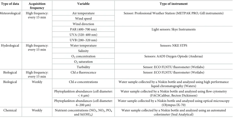
For the meteorological parameters (Table 1), air temperature, wind speed and direction, photosynthetically active radiation (PAR, 400–700 nm) and ultraviolet radiation A and B (UVA, 320–400 nm, and UVB, 280–320 nm) were recorded at a high frequency (every 15 min) using a Professional Weather Station (METPAK PRO, Gill instruments) with PAR, UVA and UVB sensors (Skye Instruments).

For the water properties at mid-depth (Table 1), the water temperature and salinity were recorded with an NKE STPS sensor (Table 1). The dissolved O2concentration and saturation

were recorded using an optical sensor (AADI Oxygen Optode, Aanderaa). The turbidity and thein situ Chl a fluorescence were recorded with an ECO FLNTU fluorometer (Wetlabs).

Water properties were recorded at the same frequency and over the same periods as the meteo-rological parameters, except for water temperature and conductivity in 2016, where the moni-toring started ten days later (from December 11, 2015, to July 6, 2016). All sensors were calibrated before deployment. The temperature sensor was calibrated from 5 to 25˚C in 5˚C steps using a reference thermometer and thermostatic bath. The salinity sensor was calibrated at 25˚C using seawater standards of 10, 30, 35 and 38 (Linearity Pack, OSIL, UK). The 0 stan-dard was made with ultrapure water (MilliQ). The oxygen sensor was calibrated at 0% and 100% O2saturation using the Winkler method [33] for measuring the O2concentration. The

Chla fluorescence sensor was calibrated using several types of phytoplankton cultures at

vari-ous concentrations, with the concentrations measured by spectrofluorometry. All sensors were

Fig 1. Location of the sampling station.

cleaned weekly to prevent biofouling, and measurement drift was checked after each measure-ment campaign using the same methods as those used to calibrate each sensor.

Weekly monitoring of nutrients, Chl

a concentrations, phytoplankton

abundance and diversity

In addition to high-frequency monitoring, water samples were collected weekly to determine nutrient and Chla concentrations and phytoplankton abundances and diversity (Table 1). Samples were collected using a Niskin bottle 1 m below the surface from January 15 to May 12, 2015, and from January 12 to July 6, 2016, between 09:00 and 10:00 am.

To determine the nutrient concentrations, 50 mL seawater subsamples were taken using acid-precleaned polycarbonate bottles and then filtered through Gelman 0.45μm filters that had been prewashed three times. Then, 13 mL of the filtrate was stored at -20˚C until analysis. Nitrate (NO3), nitrite (NO2), phosphate (PO4) and silicate (Si(OH)4) concentrations were

measured using an automated colorimeter (Seal Analytical) following standard nutrient analy-sis methods [34].

To determine Chla concentrations, 1 L subsamples were taken, filtered through glass fiber

filters (GF/F Whatman: 0.25 mm, nominal pore size: 0.7μm), and stored at -80˚C until analy-sis. Pigment concentrations, including Chla concentrations, were measured by high

perfor-mance liquid chromatography (HPLC, Waters) following the extraction protocol described in Vidussi et al. (2011) [34] and the HPLC method described by Zapata et al. (2000) [35].

Phytoplankton (< 6μm) abundances were estimated by flow cytometry (FACSCalibur, Becton Dickinson), and phytoplankton (6–200μm) abundances and diversity, by optical

Table 1. Type and acquisition characteristics of the studied variables. Type of data Acquisition

frequency

Variable Type of instrument

Meteorological High frequency: every 15 min

Air temperature Sensor: Professional Weather Station (METPAK PRO, Gill instruments) Wind speed

Wind direction

PAR (400–700 nm) Light sensors: Skye Instruments

UVA (320–400 nm) UVB (280–320 nm) Hydrological High frequency:

every 15 min

Water temperature Sensors: NKE STPS

Salinity

O2concentration Sensors: AADI Oxygen Optode (Anderaa)

O2saturation

Turbidity Sensor: ECO FLNTU fluorometer (Wetlabs)

Biological High frequency: every 15 min

Chla fluorescence Sensor: ECO FLNTU fluorometer (Wetlabs)

Biological Weekly Chla concentrations Water sample collected by a Niskin bottle and analyzed using high performance liquid chromatography (Waters)

Phytoplankton abundances (cell diameter:

< 6μm)

Water sample collected by a Niskin bottle and analyzed using flow cytometry (FACSCalibur, Becton Dickinson)

Phytoplankton abundances (cell diameter: 6–200μm)

Water sample collected by a Niskin bottle and analyzed using optical microscopy (Olympus IX-70)

Chemical Weekly Nutrient concentrations (NO3, NO2, PO4

and Si(OH)4)

Water sample collected by a Niskin bottle and analyzed using an automated colorimeter (Seal Analytical)

PAR: photosynthetically active radiation; UVA and UVB: ultraviolet A and B, respectively; O2: dioxygen;Chla: chlorophyll a; NO3: nitrate; NO2: nitrite; PO4: phosphate

and Si(OH)4: silicate.

microscopy (Olympus IX-70). For the phytoplankton (< 6μm) abundances, duplicate 1.8 mL subsamples were taken, fixed with glutaraldehyde following the protocol described in Marie et al. (2001) [36] and then stored at -80˚C until analysis. Cyanobacteria (< 1μm), picoeukar-yotes (< 3μm) and nanoeukaryotes (in this study, 3–6 μm cell diameter; seeResults) abun-dances were estimated using the flow cytometry method described by Pecqueur et al. (2011) [37]. Phytoplankton (6–200μm) abundance and diversity were estimated by microscopy. Duplicate 125 mL subsamples were taken, fixed in 8% formaldehyde and then settled for 24 h in an Utermo¨hl chamber. Cells of each identified phytoplankton taxon were counted under an inverted microscope. Phytoplankton were identified to the lowest possible taxonomic level (species or genus) using standard keys for phytoplankton taxonomy [38]. Carbon biomasses of phytoplankton analyzed by flow cytometry were estimated using the conversion factors of 0.21 pgC cell-1for cyanobacteria and 0.22 pgCμm-3for picoeukaryotes and nanoeukaryotes [39]. For microscopic observations, phytoplankton biovolumes were estimated for the most com-mon taxa using the best shape [40], and carbon biomasses were then calculated using the con-version factors [41,42].

Chl

a fluorescence correction and bloom identification

Chla fluorescence is commonly used as a proxy for phytoplankton biomass. Chl a

fluores-cence data from the fluorometer were corrected using the weekly measurements of Chla

con-centrations by HPLC to provide coherent high-frequency Chla fluorescence data [43]. Bloom periods were identified by estimating the net phytoplankton growth rate (Eq 1) using the biomass gain or loss [5,9]. The high-frequency Chla fluorescence data over 24 h

were used to calculate the daily mean phytoplankton biomass (Ct). The daily net growth rate

(rt) was the difference in phytoplankton biomass between two consecutive days. A negative

value indicates a biomass loss, whereas a positive r value indicates a biomass gain.

rtþ1¼Ctþ1 Ct ð1Þ

A bloom was identified as a period 1) that started with at least 2 consecutive days of positive growth rates and 2) where the sum of net growth rates over at least 5 consecutive days was pos-itive. The end of the bloom was the day before 5 consecutive days with negative growth. A 1-day peak of net growth was considered a “sporadic event” and not a bloom. When close suc-cessions of 5-day blooms were identified, they were coalesced into “bloom periods” followed by “post-bloom periods” to identify key events. The means of the daily net growth rates were calculated for bloom periods to compare the mean growth rates among the different periods.

Data analysis

Some of the operations required to maintain the quality of the high-frequency sampling, such as sensor recalibration and cleaning or drift correction, occasionally induced single or multiple missing measurements or outliers, which were removed from the data set. In our study, the fraction of missing values for each variable was generally low, i.e., between 0.06% (water tem-perature, 2015) and 23.48% (O2saturation, 2016). Only the UVA data in 2016 had a higher

rejection rate (61.96%), due to a technical problem. Consequently, UVA data were not included in the data analysis for 2016 but were included in the 2015 analysis. All the other missing high-frequency data were estimated using a moving average in a 480 data point win-dow (5 days) [44].

The daily mean of the high-frequency data except for PAR, UVA and UVB was calculated to remove daily variation patterns; for the three exceptions, the daily cumulative value was cal-culated. The whole data set (i.e., daily values of biological, meteorological and hydrological

data) was kept as a separate set for each study period. The two resulting data sets were divided into separate data sets for each period as bloom periods (winter, early spring and spring), post-bloom periods (post-winter post-bloom and post-early spring post-bloom) and a winter latency period. The winter latency period was defined as a period where the daily net growth rate was low, with a mean daily net growth rate close to zero. A post-spring bloom in 2015 and a pre-winter bloom in 2016 were identified. However, these blooms were too short to perform a strong sta-tistical test; therefore, we did not keep them in the analysis of identified periods. These separa-tions between different periods therefore provided therefore 5 data sets for 2015 and 4 data sets for 2016. Then, autoregressive and moving average (ARMA) models were used for each time series in each data set to identify ARMA processes [45] before first-differencing the fitted series to remove stationarity [46]. Principal component analysis (PCA) was used on the fitted and first-differenced time series in the 2015 and 2016 data sets to identify the relationships between environmental variables graphically. Then, Spearman’s rank correlation tests were applied pairwise to highlight significant correlations in the 2015 and 2016 data sets. As Chla

may exhibit a delayed response to environmental forcing factors, time-lag correlation tests were performed on the 11 different data sets. Time-lag correlations are based on simple Spear-man’s rank correlation tests between two variables repeated with time-shifted data to identify the delayed influence of a variable on the Chla dynamics.

The weekly data (nutrient concentrations and phytoplankton abundances and diversity) were kept as a separate data set for each study period but were not divided into identified peri-ods because the quantity of data would have been insufficient (19 data points for 2015 and 23 data points for 2016). For the high-frequency data, ARMA models were used for each time series in each data set when needed. Paired Wilcoxon signed-rank tests were used to compare the mean values of the phytoplankton abundances and diversity and the nutrient concentra-tions between the 2015 and 2016 data sets. Sample dates were paired by week number (ISO 8601). For example, the sampling dates of January 8, 2015, and January 12, 2016, both corre-sponding to the 2ndweek of the year, were paired. To identify correlations between weekly data and high-frequency environmental data, daily means of the environmental data for the sampling days were added to the weekly data sets before using ARMA models and first-differencing each time series. Spearman’s rank correlation tests were then performed pairwise on the 2015 and 2016 data sets.

Results

Bloom identification based on Chl

a fluorescence data

Three blooms were identified in 2015, while only two blooms were identified in 2016 (Fig 2A and 2B). Blooms were defined as consecutive days of biomass gain (positive values of daily net growth rates), while post-bloom periods were consecutive days of biomass loss (negative val-ues;Fig 2C and 2D, respectively). There were winter blooms in January for 2015 and one month earlier, in December 2015, for 2016 (Fig 2A and 2B). The 2016 winter bloom was stron-ger, with Chla concentrations reaching 3.64 μg L-1in 2016 and 2.77μg L-1in 2015 (Fig 2A and 2B) and maximum daily net growth rates of 0.54μg L-1in 2016 and 0.49μg L-1in 2015 (Fig 2C and 2D). The mean daily net growth rate was 0.055μg L-1d-1in 2016, almost double the 0.031μg L-1d-1in 2015. However, it should be noted that the 2015 winter bloom had already started at the beginning of the monitoring. The winter blooms in 2015 and 2016 were followed by post-bloom periods, with the Chla concentration falling to 0.54 μg L-1in 2015 and 0.62μg L-1in 2016. In 2015, there was an early spring bloom between February 11 and March 11 that was weaker than the preceding winter bloom (maximum Chla: 2.01 μg L-1and mean daily net growth rate: 0.023μg L-1d-1). This early spring bloom was followed by a post-bloom period,

with the Chla concentration falling to 0.54 μg L-1. In 2016, however, instead of an early spring bloom, there was a winter latency period from January 6 to March 11. During this period, the daily net growth rates were low (Fig 2D), with a mean daily net growth rate close to zero. Then, the main spring blooms occurred from April 9 to May 14 (36 days) in 2015 and from March 24 to July 05 (104 days) in 2016. Notably, the monitoring periods had been planned to end on May 19, 2015, and July 6, 2016; therefore the spring blooms might have continued after these dates. In 2016, the spring bloom showed a maximum Chla concentration of 3.16 μg L-1, which was higher than the value of 2.93μg L-1recorded in 2015, but with a mean daily net growth rate (0.010μg L-1) d-1lower than that (0.022μg L-1) d-1recorded in 2015.

High-frequency meteorological and hydrological data

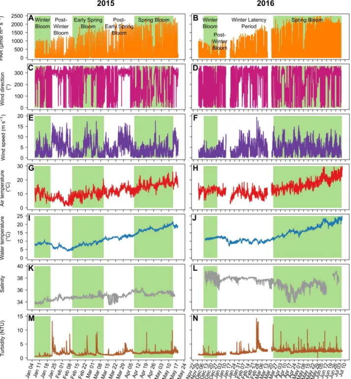
The PAR was lowest when the winter blooms occurred in both 2015 and 2016 (Fig 2A and 2B). Then, the PAR slowly increased to reach its maximum of 2688μmol m2s-1on April 19, 2015, and 2865μmol m2s-1on June 18, 2016.

Two dominant winds were identified. Dominance of wind was based on the frequency of occurrence of wind directions over the two studied periods (Fig 3C and 3D). The first wind was from the northwest (49.5% of the data between 270˚ and 359˚), and the second was from the southeast (21% of the data between 90˚ and 180˚). There were three windy periods with northwesterly winds (median of 302˚) in 2015 (Fig 3E) during the post-winter bloom period (max = 16.6 m s-1), the early spring bloom period (max = 17.4 m s-1) and the post-early spring bloom period (max = 16.5 m s-1). The wind speed was lower during the winter bloom, the onset of the early spring bloom and the spring bloom (means of 3.3, 1.9 and 3.1 m s-1,

respectively). In 2016 (Fig 3F), the wind speeds were low during the winter bloom (mean = 1.8

Fig 2. Chlorophylla fluorescence and daily net growth rates. In situ Chl a fluorescence in 2015 (A) and 2016 (B) and daily net growth rates in 2015

(C) and 2016 (D), indicating daily biomass gains (positive values) and losses (negative values). The bloom periods have a green background, and the post-bloom periods and winter latency period have a white background.

m s-1); otherwise, the wind was erratic, with numerous short windy events exhibiting mean wind speed values higher than those observed during the winter bloom.

During the 2015 study period, the mean air temperature dropped from 19.9˚C in early Jan-uary to 1.1˚C in early FebrJan-uary (Fig 3G). It then increased until the end of the study period,

Fig 3. Environmental variables. Main environmental variables for 2015 (left) and 2016 (right). A to H are the meteorological data: PAR (A and B),

wind direction (C and D), wind speed (E and F) and air temperature (G and H); and I to N are the hydrological variables: water temperature (I and J), salinity (K and L) and turbidity (M and N). The background colors for the various periods are the same as inFig 2.

with a maximum of 25.7˚C on May 14. During the 2016 study period, the air temperature was stable from early December to mid-March (mean: 10.9±2.7˚C, minimum: 2.9˚C and maxi-mum: 18.5˚C) with a quick chill in early January (Fig 3H). Then the air temperature increased from mid-March until the end of the study period, with a maximum of 30.8˚C on July 7.

The water temperature was less variable than the air temperature (Fig 3I and 3J). In 2015, the water temperature was stable during January (8.5±0.6˚C), decreased to a minimum of 4.0˚C on February 6 and then increased to 21.7˚C on May 14. In 2016, the water temperature was 11.8±0.5˚C from December 12 to January 11, followed by a quick chill to a minimum of 7.0˚C on January 17. Then, the water temperature was stable until March 10 (9.9±0.8˚C), fol-lowed by an increase until the end of the study period, reaching a maximum of 25.1˚C on July 6.

The salinity was also different between 2015 and 2016 (Fig 3K and 3L). In 2015, the salinity was 34.95±0.56, while in 2016, it was higher (37.34±0.95) and more variable and exhibited a large decrease during April, reaching a minimum value of 33.85 on April 18.

The turbidity (Fig 3M and 3N) was 1.69±0.87 NTU in 2015, which was lower than the 2.25 ±1.06 NTU observed in 2016, with sporadic peaks reaching 13.15 NTU in 2015 and 14.19 NTU in 2016.

Relationships between Chl

a fluorescence, meteorological and hydrological

data

The general relationships between Chla, meteorological and hydrological data in 2015 and

2016 based on PCA are shown inFig 4A and 4B. For both data sets, there was a group on the second axis, comprising the wind conditions (speed and direction) and turbidity. Spearman’s rank correlations were strong between wind speed and wind direction for both data sets (2015: ρ = 0.38, p-value < 0.001; 2016: ρ = 0.48, p-value < 0.001). However, the turbidity was corre-lated with the wind conditions in 2015 (speed:ρ = 0.41, value < 0.001; direction: ρ = 0.19, p-value < 0.05) but not in 2016. Another group, on the first PCA axis of both data sets, com-prised the light parameters, i.e., PAR, UVA (only in 2015) and UVB, and oxygen concentration and saturation. Spearman’s rank correlations were significant between light conditions and oxygen (2015: allp-values < 0.01; 2016: all p-values < 0.001). Chl a fluorescence was opposed

to both these groups in both 2015 and 2016, with significant negative correlations with the wind conditions (allp-values < 0.05) and the light conditions (all p-values < 0.05). The PCA

for both data sets also showed a positive correlation between water temperature and air tem-perature (2015:ρ = 0.36, p-value < 0.001; 2016: ρ = 0.29, p-value < 0.001). The water tempera-ture was positively correlated with Chla fluorescence in 2015 (ρ = 0.25, p-value < 0.01) but

not in 2016.

Time-lag correlations between high-frequency Chl

a fluorescence,

meteorological and hydrological data

As Chla fluorescence may have exhibited a delayed response to environmental forcing factors,

the time series were tested for time-lag correlations (Table 2). Chla fluorescence was positively

correlated with the water temperature (0- and 5-day lags, strongp-values < 0.01) as well as

salinity (1- and 3-day lags,p-values < 0.05) in both the 2015 and 2016 data sets. As found

using PCA, Chla fluorescence was negatively correlated with the light conditions (PAR, UVA

and UVB), with a 0-day lags in both 2015 and 2016. However, there was a positive correlation between Chla fluorescence and light conditions with a 1-day lag, but only in 2015. There were

negative correlations between Chla fluorescence and wind conditions (speed and direction)

For the separate periods (bloom, post-bloom and winter latency periods), Chla

fluores-cence was positively correlated with water temperature, with a lag of from 0 to 5 days during four of the five bloom periods (p-values from < 0.05 to < 0.001). Chl a fluorescence was

nega-tively correlated with the wind conditions (speed and/or direction), with a range of lags between 0 and 4 days for four blooms (p-values from < 0.05 to < 0.001). Salinity was positively

correlated with Chla fluorescence during the early spring bloom in 2015 (p-value < 0.001)

and negatively correlated with Chla fluorescence during the winter bloom in 2016

(p-value < 0.001). Chla fluorescence was negatively correlated with light conditions for 3 blooms

with 0-day lags (p-values from < 0.05 to < 0.001), while for the spring bloom in 2015, they

were positively correlated with a 1-day lag (p-value < 0.05). There was little correlation during

the post-bloom periods. Chla fluorescence was negatively correlated with PAR and UVA

dur-ing the post-winter bloom in 2015 (5-day lags,p-value < 0.05) as well as with the wind speed

in for 2016 (0-day lag,p-value < 0.05) and was positively correlated with the wind direction

(5-day lags,p-value < 0.05) during the post-early spring bloom period in 2015.

Nutrient dynamics

During the winter bloom and the post-winter bloom periods, the PO4, NO2and NO3

concen-trations were on average 3 to 9 times lower in 2015 (0.01±0.00, 0.07±0.03 and 0.72±0.24 μmol L-1, respectively) (Fig 5A, 5E and 5G) than in 2016 (0.09±0.05, 0.20±0.05 and 2.26±0.63 μmol L-1, respectively) (Fig 5B, 5F and 5H). The Si(OH)4concentration (Fig 5C and 5D) in 2015

(8.67±2.05 μmol L-1) was, however, twice that in 2016 (3.86±0.57 μmol L-1) over the same period. In 2015, the Si(OH)4concentrations then gradually decreased until the end of the early

spring bloom, reaching a mean of 2.14±0.29 μmol L-1in March.

Fig 4. Principal component analysis (PCA) of environmental variables. PCA of Chla, meteorological and hydrological data for the 2015 data set (A)

and 2016 data set (B). PCA allows the variables to be projected in multidimensional space to highlight the relationships between them. Here, only two dimensions are represented as they explain the environmental dynamic well. The arrows represent the variables. When arrows are far from the center and close to each other, they are positively correlated, whereas when they are symmetrically opposed, they are negatively correlated. If the arrows are orthogonal, they are not correlated. Finally, when the variables are close to the center, they are not well projected in the dimensions represented; consequently, it is hard to conclude that a relationship occurs between these variables. In this last case, to highlight masked links, we coupled the PCA with pairwise Spearman’s rank correlations as described in the Material and methods.

In 2015, from the early spring bloom to the end of the spring bloom, the PO4, NO2and

NO3concentrations remained at the same levels as in the winter, even though there were

peaks in the PO4(0.08μmol L-1) and NO3(6.01μmol L-1) concentrations on March 12. In

2016, over the same period, the PO4, NO2and NO3concentrations fluctuated more than

in 2015, but the mean values were similar (0.04±0.06, 0.04±0.02 and 1.24±0.83 μmol L-1, respectively). The mean Si(OH)4concentration during the spring bloom in 2015 (1.62

±1.00 μmol L-1) was approximately half that in 2016 (2.74±0.80 μmol L-1).

Wilcoxon signed-rank tests showed that the PO4and NO3concentrations were significantly

higher in 2016 than in 2015 (p-values < 0.05). The N:P ratios (Redfield ratios) were between

11 and 94 (mean: 45±25) in 2015 and between 6 and 124 (mean: 46±35) in 2016. Spearman’s rank correlations showed significant correlations between Chla and nutrient concentrations

in neither 2015 nor 2016.

Dynamics of phytoplankton abundances

Three groups of picophytoplankton, namely, cyanobacteria (< 1μm diameter), picoeukaryotes (< 1μm diameter) and picoeukaryotes (1–3 μm diameter), and one group of nanoeukaryotes (3–6μm diameter) were enumerated by flow cytometry (Fig 6A to 6D). The abundances of picoeukaryotes (< 1μm and 1–3 μm) and nanoeukaryotes were similar between 2015 and 2016: the total abundance of these three groups was 2.14±1.30 × 104cells mL-1in 2015 and 2.84±1.41 × 104cells mL-1in 2016. However, the mean abundance of picoeukaryotes and

Table 2. Time-lag correlations between meteorological and hydrological data. Year Period PAR UVA UVB Wind

speed Wind direction Air temperature Water temperature Salinity Turbidity 2015 Whole - - (0;0.27) + + + (1;0.31) - - (0;0.24) + + + (1;0.32) - (0;0.22) + + + (1;0.31) - (0;0.17) - - (1;0.28) - - (0;0.24) + + (0;0.25) + (3;0.18) Winter Bloom + + (0;0.71) - - (4;0.79) Post-Winter Bloom - (5;0.56) - (5;0.55) + (3;0.54)

Early Spring Bloom - (0;0.40) - (0;0.39) + (5;0.43) + + + (0;0.60) + + +

(0;0.56) - (4;0.43) - (0;0.38) Post-Early Spring Bloom + (5;054) Spring Bloom - (0;0.41) + (1;0.39) - - (0;0.43) + (1;0.41) - (0;0.41) + (1;0.39) + (2;0.40) - - (0;0.53) + (2;0.35) 2016 Whole - - - (0;0.38) - - - (0;0.36) - (0;0.17) - (2;0.30) - - (0;0.30) - (2;0.15) + + (5;0.17) + (1;0.15) ++ (3;0.21) + (0;0.16) Winter Bloom - - (0;0.57) + (0;0.54) - - - (0;0.72) Post-Winter Bloom - (0;0.86) Winter Latency Period - (0;0.25) + + (3;0.32) - - (0;0.31) + + (3;0.34) - (0;0.24) + + (4;0.32) + + (3;0.32) + + (0;0.35) - - (1;0.32) Spring Bloom - - - (0;0.44) - - - (0;0.44) -(0;0.35) + (5;0.21) - - (0;0.27) - (1;0.22) + (5;0.23) - (0;0.25) - (2;0.20) + (5;0.21)

Spearman’s rank time-lag correlations between Chla fluorescence and environmental variables in 2015 and 2016. Whole: tests performed on the whole data set for a

study period. Only significant results are shown. The signs + and—represent significant positive and negative correlations, respectively; a single sign represents

p-value < 0.05; ++ or—representsp-value < 0.01; and +++ or—represents p-value < 0.001. The time lag (in days) and coefficient of the correlations are in parentheses.

For example, +(2;0.40) represents a positive correlation with ap-value < 0.05, 2-day lag and coefficient of 0.40. The bloom periods have a green background.

nanoeukaryotes during the spring bloom in 2016 (6.53±1.38 × 104cells mL-1) was more than twice that in 2015 (2.84±1.73 × 104cells mL-1). One of the main differences between 2015 and 2016 was that during winter and early spring, the cyanobacteria (< 1μm) abundance in 2016 (2.19±2.19 × 103cells mL-1) was almost 10 times higher than that in 2015 (3.02±2.55 × 102 cells mL-1). Then, during the spring bloom, cyanobacteria abundances increased to a maxi-mum on May 06, 2015 (6.01× 104cells mL-1), and a lower maximum on May 10, 2016 (2.70× 104cells mL-1). The Wilcoxon signed-rank test showed that the mean abundances of cyanobacteria (p-value < 0.01), picoeukaryotes (< 1 μm) (p-value < 0.01) and nanoeukaryotes

Fig 5. Nutrient concentrations. Nutrient concentrations in 2015 (left) and 2016 (right) for PO4(A and B), Si(OH)4(C and D), NO2(E and F), and

NO3(G and H). The background colors for the various periods are the same as inFig 2.

(p-value < 0.05) were significantly higher in 2016 than in 2015, but there was no significant

difference for picoeukaryotes (1–3μm). Tests for correlations between the biological variables (picophytoplankton and nanophytoplankton abundances and Chla fluorescence) and the

environmental variables (wind conditions, light conditions, salinity, air and water tempera-ture, oxygen, turbidity and nutrients) showed a negative correlation of picoeukaryotes (1– 3μm) with PO4concentrations in 2015 (ρ = -0.54, p-value < 0.05) and with NO3in 2016 (ρ =

-0.50,p-value < 0.05). Picoeukaryotes (< 1 μm) were negatively correlated with wind

condi-tions in 2015 (wind speed:ρ = -0.57, p-value < 0.05; wind direction: ρ = -0.50, p-value < 0.05). The patterns of community composition and total abundances of phytoplankton (6– 200μm) were different between 2015 and 2016 (Fig 6E to 6J). The total abundances of phyto-plankton (6–200μm) were quite similar during winter and early spring in 2015 (266±81 cells mL-1) and 2016 (212±91 cells mL-1). During the spring bloom, however, the total phytoplank-ton (6–200μm) abundances in 2015 were almost three times those in 2016 (982±433 cells mL

-1

and 378±123 cells mL-1, respectively). This result was confirmed by the Wilcoxon signed-rank test showing that total phytoplankton abundances (6–200μm) were significantly higher in 2015 than in 2016 (p-value < 0.01). The maximum abundances of phytoplankton (6–

200μm) were reached on May 6, 2015, and June 8, 2016 (1470 cells mL-1and 923 cells mL-1, respectively). In 2015, during the winter and early spring blooms and their post-bloom

Fig 6. Phytoplankton abundances and diversity. Analyzed by flow cytometry for 2015 (A and C) and 2016 (B and D). Dominant taxa observed by

microscopy for 2015 (E, G and I) and 2016 (F, H and J). The background colors for the various periods are the same as inFig 2. https://doi.org/10.1371/journal.pone.0214933.g006

periods, the phytoplankton community was dominated numerically byPlagioselmis prolonga,

a cryptophyte with a diameter of 8–12μm (41±13%), and chlorophytes (~6 μm) (38.0±8.5%). In addition, chrysophyceae (~6μm) were also abundant during the early spring bloom (18 ±2%). In 2016, P. prolonga dominated the phytoplankton (6–200 μm) community during the winter latency period and the first 11 weeks of the spring bloom (48±11%), and chlorophytes (~6μm) were also abundant but less abundant than in 2015 (29±9%). Pseudo-nitzschia sp. (25–50μm) and Chaetoceros spp. (10–50 μm), which are large, colonial diatoms, successively dominated the phytoplankton (6–200μm) community during the spring bloom in early April 2015 (72±13%) and the second part of the spring bloom from mid-May 2016 (65±23%) until the end of the study periods.Chaetoceros spp. abundances were significantly lower in 2015

than in 2016 (Wilcoxon signed-rank test,p-value < 0.05), but Pseudo-nitzschia sp. abundances

were not.

The phytoplankton community was dominated numerically by picoeukaryotes (< 1μm), accounting for 51 to 95%, depending on the period (Table 3). However, in terms of carbon bio-mass, picoeukaryotes were never dominant. In 2015, the carbon biomass was dominated byP. prolonga in the winter and early spring blooms and by Chaetoceros spp. in the spring bloom.

Nanoeukaryotes contributed most of the carbon biomass throughout 2016.

Correlations between weekly measurements of phytoplankton abundances (6–200μm), Chl

a fluorescence and environmental variables were calculated separately for 2015 and 2016. In

2015,P. prolonga abundance (ρ = -0.60, p-value < 0.05) was negatively correlated with PO4

concentration, andChaetoceros spp. abundance was positively correlated with Chl a

fluores-cence (ρ = 0.67, p-value < 0.01). In 2016, Pseudo-nitzschia sp. abundance was positively corre-lated with Chla fluorescence (ρ = 0.55, p-value < 0.05), and Chaetoceros sp. abundance was

positively correlated with NO3concentration (ρ = 0.58, p-value < 0.01).

Discussion

Role of water temperature and winter cooling in phytoplankton blooms

Based on the time-lag correlations, water temperature played a significant role in determining Chla dynamics, especially the onset of blooms (Table 2). This is the first time that rising water temperature has been identified as the main factor triggering phytoplankton blooms in an aquatic ecosystem (ocean, coastal zone or lake). This relationship was true for all the main blooms observed in 2015 and 2016, and the strength, number of occurrences and consistent positive sign of the correlations between water temperature and Chla fluorescence suggested

that water temperature was the main driver. Other parameters such as wind conditions and salinity were correlated with blooms (see below) but the number of occurrence and non-con-sistent sign of the correlations suggested that they were not the main drivers. The water tem-perature was positively correlated with Chla fluorescence with 0 to 5 days of lag suggesting

that the biomass accumulation represented by increasing Chla fluorescence was driven by the

increase in water temperature over the 5 previous days. Furthermore, every bloom onset corre-sponded to a period of increase in water temperature, while such correspondence was not detected for other parameters.

The effect of temperature on phytoplankton physiology and metabolic processes is well known. First, under light-saturated conditions, higher temperature increases specific phyto-plankton productivity by acting on photosynthetic carbon assimilation [47,48]. In addition, under non-limiting nutrient conditions, an increase in water temperature increases phyto-plankton nutrient uptake [49,50]. Moreover, phytoplankton growth rates increases with increasing of temperature, almost doubling with each 10˚C increase in temperature (Q10

of herbivorous grazers at low temperatures [51,52]. Thus, an increase in water temperature, particularly at relatively relative lowin situ temperatures such as those in this study (6–14˚C),

can be more favorable for phytoplankton than for their grazers, allowing phytoplankton mass accumulation, which starts the bloom. Therefore, the initiation of phytoplankton bio-mass accumulation can result from phytoplankton growth temporarily exceeding grazing-induced losses as a result of increasing temperature.

In previous studies, water temperature was identified as the main driver of blooms of par-ticular species, especially cyanobacteria [53,54]. However, the present study underlined that an increase in water temperature triggered blooms of all phytoplankton community blooms, not just a particular species. Furthermore, the spring blooms started at a temperature of 13.9˚C in 2015 and 11.2˚C in 2016, while the early spring bloom in 2015 began when the water tempera-ture was 6.1˚C. This wide water temperatempera-ture range for bloom initiations indicates that there is not a threshold water temperature that triggers phytoplankton blooms; instead, blooms are ini-tiated by an increase in water temperature.

Interannual comparison showed that winter 2015/2016 was the warmest winter recorded in France according to Meteofrance ( http://www.meteofrance.fr/climat-passe-et-futur/bilans-climatiques/bilan-2016/hiver), which led to exceptionally high winter water temperatures. In contrast in 2015, the winter cooling of the water was typical of this coastal site. As a result, the Chla dynamics in 2016 were completely different from those in 2015 (Fig 1). The absence of an early spring bloom and the slower biomass accumulation during the 2016 spring bloom can be explained by the difference between the meteorological conditions. The abnormally high water temperature during the 2016 winter may have been the cause of biomass stagnation dur-ing the winter latency period, slowdur-ing phytoplankton biomass accumulation durdur-ing the sprdur-ing. The absence of significant winter cooling and the relatively mild water temperatures may have allowed predators (e.g., ciliates and copepods) as well as filter feeders (e.g., oyster and mussels) to remain active during this period and maintain grazing pressure on the phytoplankton [55,56], in turn delaying the ecosystem disturbance required to start a bloom until mid-March, when the water temperature started to rise. Therefore, winter water temperature seems to be a crucial factor influencing the dynamics of the spring bloom in temperate shallow coastal zones. The effect of the winter water temperature on the magnitude of the spring bloom has already been reported [57,58], with larger spring blooms and more phytoplankton biomass after cold winters and smaller spring blooms after mild winters in the Wadden Sea. With

Table 3. Relative contributions of the dominant phytoplankton groups to the carbon biomass and abundance.

2015 2016

Winter Bloom Post-Winter Bloom

Early Spring Bloom

Post-Early Spring Bloom

Spring Bloom Winter Latency Period Spring Bloom C Ab C Ab C Ab C Ab C Ab C Ab C Ab Cyanobacteria (< 1μm) 0.17 0.62 0.54 0.89 0.38 1.54 1.10 1.92 7.81 40.60 3.48 6.83 5.67 19.82 Picoeukaryotes (< 1μm) 6.86 90.50 16.03 94.74 5.49 79.06 14.43 89.49 2.78 51.43 12.38 86.50 5.45 67.86 Picoeukaryotes (1–3μm) 4.81 4.07 8.60 3.25 15.05 13.88 16.49 6.54 3.62 4.29 7.96 3.56 9.73 7.75 Nanoeukaryotes (3–6μm) 28.52 3.01 13.44 0.64 35.26 4.06 28.87 1.43 14.26 2.11 46.23 2.59 39.87 3.97 Plagioselmis prolonga 31.99 0.92 19.02 0.24 37.41 1.17 27.93 0.38 4.50 0.18 22.43 0.34 6.77 0.18 Chlorophytes 14.68 0.81 5.61 0.14 4.63 0.28 9.11 0.23 1.58 0.12 5.91 0.17 2.69 0.14 Chaetoceros spp. 12.97 0.08 36.76 0.10 1.78 0.01 1.92 0.01 52.96 0.45 1.43 0.00 27.31 0.17 Pseudo-nitzschia sp. 0.00 0.00 0.00 0.00 0.00 0.00 0.14 0.00 12.48 0.82 0.17 0.00 2.50 0.11 Mean relative contribution (in percent) to the carbon biomass (CB) and numerical abundance (Ab) of the dominant phytoplankton groups during each period. Species and period abbreviations and background colors are the same as inTable 2. The highest contribution for each period is in bold.

global warming, these mild winters could become more frequent [59] and may reduce phyto-plankton biomass accumulation during spring blooms. This modification of the bloom phe-nology might potentially change the structure of the plankton community assemblages and, therefore, directly affect the food web. Such modification is particularly important in shallow temperate coastal zones of economic interest as changes in bloom phenology and magnitude may affect fish and shellfish production.

There were short (2–3 weeks) winter blooms in both 2015 and 2016. Winter blooms are known to occur in marine ecosystems, but they are less common than spring blooms. Winter blooms can be rare, exceptional events [60], but they may occur regularly every year, as in the Bahia Blanca Estuary in Argentina [61] or in tropical and subtropical seas [62–64]. Winter blooms in the coastal site of the present study were recorded once before, in December 1993 [65,66], whereas the present study documented winter blooms of a magnitude similar to that of the spring bloom in two consecutive years. These winter blooms represent an important part of annual primary production (daily mean net growth rates of 0.055μg L-1

d-1in 2015 and 0.031μg L-1d-1in 2016), providing food for the whole plankton food web, and can sometimes be the most important biomass accumulation event during the year [61]. Winter blooms in shallow coastal zones are generally triggered by a combination of forcing factors such as high nutrient concentrations due to autumn rains, an increase in light penetration into the water column due to a reduction in suspended matter or sediments and low grazing pressure due to low water temperature or tidal conditions [61]. In this study, water temperature was associated with the increase in Chla fluorescence during the winter bloom of 2016. For 2015, however,

the winter bloom had already been triggered when the monitoring started, and the link between water temperature and Chla for this winter bloom could not be established as the

time-lag correlations could not be determined. Additional observations will be necessary to establish whether an annual winter bloom has become a rule, which might indicate that an ecological shift has occurred in this system. The winter bloom may also have been the result of particular climatic/environmental conditions that occurred during the study period. In fact, even though the impact of the El Niño-Southern Oscillation (ENSO) on the Mediterranean cli-mate is still a source of discussion [67], 2015 was a strong El Niño year with an ENSO Oceanic Niño Index (ONI) value of approximately 2, making it less important than that in 1997–1998 but more than that in 1991–1992 [68], which could potentially explain the exceptional 2015– 2016 winter climatic conditions.

Role of other environmental forcing factors in phytoplankton blooms

Nutrient input from runoff, rain events or sediment resuspension is widely considered a key factor triggering blooms in coastal zones. However, there was no direct link between nutrient concentrations and Chla fluorescence in this study, suggesting that nutrients are not the sole

driver of Chla dynamics and that a more complex functioning drives blooms in this

mesotro-phic system (Fig 5). The absence of a link with nutrient concentrations could be explained by the meteorological conditions of this shallow coastal system, where the wind causes a fairly constant nutrient supply from sediment resuspension, which can maintain the necessary nutrient level for phytoplankton growth but does not produce inputs large enough to reveal show a direct link. The wind conditions (speed and direction) were correlated with Chla

fluo-rescence with 0- to 5-day lags throughout the study periods and during three bloom periods each (Table 2). These correlations may indicate that high-speed winds, generally from the northwest (the tramontane, Figs3and4), reduce biomass accumulation, while low-speed winds, generally from the east and southeast increase biomass accumulation. Millet and Cecchi (1992) [69] already reported this relationship between wind conditions and Chla dynamics in

this shallow coastal lagoon. They suggested that a wind speed of 4 m s-1was optimal for balanc-ing the beneficial effect of vertical turbulent diffusion and the detrimental influence of hori-zontal advection dispersion. In our study, wind speed was significantly correlated with turbidity, which was probably caused by sediment resuspension (in particular, peaks of wind speed coincided with those of turbidity,Fig 3), as has already been reported for shallow coastal zones [65,70,71]. This sediment resuspension, creating a fairly constant nutrient input to the water column, may have maintained phytoplankton production and biomass. With weekly nutrient sampling, the role of nutrient inputs in bloom dynamics may be masked because phy-toplankton communities respond quickly to nutrient inputs [72]. The use of high-sensitivityin situ nutrient sensors with high acquisition frequencies is crucial for improving our

under-standing of the effect of nutrient inputs on blooms in such dynamic systems.

There were some correlations between phytoplankton group abundances and nutrient dynamics, especially for PO4. Furthermore, the N:P ratio was almost 3 times the Redfield ratio

of 16:1, suggesting that PO4could be a limiting factor for some phytoplankton groups during

some periods of the year. This result is in agreement with that from a nutrient limitation study of French Mediterranean coastal lagoons [38]. In warmer conditions, as the metabolic demands per unit biomass increase, a higher nutrient supply is needed to support phytoplank-ton growth. As the nutrient demand increases, stress and competition for nutrients increase and smaller phytoplankton benefit [55,73]. However, the PO4and NO3concentrations were

higher in 2016, especially during the winter latency period. This result supports our hypothesis that the predators remain active because of mild water temperatures, in turn maintaining a high grazing pressure and leading to low levels of phytoplankton biomass and thus lower nutrient consumption.

Chla fluorescence and salinity were correlated two times during blooms. Increases in

salin-ity in the studied system can be due to warm and dry periods inducing high evaporation or the inflow of saltier water from the Mediterranean Sea via winds. Otherwise, a decrease in salinity is generally caused by freshwater inputs from rain, runoff or floods. When the salinity varia-tions result from saltier water inflow or from freshwater inputs, nutrients may also be input [37,74]. In this study, correlations between salinity and Chla fluorescence were positive one

time (for the early spring bloom in 2015) and negative one time (for the winter bloom in 2016), suggesting that there was an indirect effect on phytoplankton biomass through nutrient inputs rather than a direct physiological effect of salinity [75]. Rain and consequent runoff events may have enriched the system with nutrients, providing a supply for phytoplankton growth. This may have been the case for the onset of the winter bloom in 2016, where a decrease in salinity was observed and corresponded to a 4-day rain event during the initiation of the bloom (https://www.historique-meteo.net). This rain event may have enriched the sys-tem with nutrients, facilitating phytoplankton growth. Additionally, saltier water inputs from the sea due to strong winds from the southeast may have led to upwelling of nutrient-rich waters or induced the transport and/or accumulation of phytoplankton in the lagoon by cur-rents. These nutrient enrichments can benefit phytoplankton growth [76,77]; however, nutri-ents can be rapidly assimilated and thus may have not been detected by our weekly nutrient sampling. Saltier water inputs can also explain the strong positive link detected between salin-ity and Chla fluorescence during the early spring bloom in 2015. The beginning of this period

was characterized by winds coming from the southeast that may have input saltier and more nutrient-rich water from the Mediterranean Sea, in turn contributing to the phytoplankton bloom. The southeasterly wind may also have prevented the dispersion of the accumulated phytoplankton.

One other important result was the lack of correlations between incident light parameters (PAR, UVA and UVB irradiance) and Chla dynamics (Table 2). This lack suggests that in the

study system, light conditions are non-limiting for phytoplankton production, at least during winter and spring. The study site is a shallow lagoon in which light reaches a large part of the water column, with a mean attenuation coefficient of 0.35 m-1[78]. In shallow temperate coastal systems, light is often non-limiting, as the light intensities in the water column are gen-erally higher than the saturating light intensities for phytoplankton growth [79]. The non-lim-iting light was also supported by the occurrence of winter blooms with similar levels of Chla

fluorescence as the spring blooms, even though the light intensities were at their lowest level (Figs2and3). Even though light did not appear to have a direct impact on Chla fluorescence

in this study, day length may have played a role in bloom timing [80]. There were also some negative correlations between incident light and Chla fluorescence with zero lag, probably

due to the inhibition of phytoplankton under high light intensities, as mentioned in the litera-ture [81,82]. Where there were positive correlations between incident light and Chla

fluores-cence, they exhibited a time lag of 1 to 3 days. One possible explanation for this result is that the phytoplankton responded, after a delay, to the high light conditions by first recovering from light inhibition and then increasing their biomass once acclimatized.

Small phytoplankton species benefit and diatoms lose out in warmer

conditions

The dominant phytoplankton species in terms of carbon biomass in the 2015 winter bloom and the early spring bloom was the cryptophyteP. prolonga (6–12 μm). Plagioselmis is a

wide-spread genus in Mediterranean coastal waters throughout the year and is sometimes consid-ered the key primary producer in these systems [83,84].Plagioselmis and cryptophytes in

general “high-quality food” [85], ensuring efficient energy transfer to higher trophic levels. In 2016, there was a winter latency period but no early spring bloom. Nanoeukaryotes (3–6μm) dominated in terms of carbon biomass during the winter latency period, with higher abun-dances than those observed in 2015, while theP. prolonga abundance was the same as that in

2015. Nanoeukaryotes (3–6μm) and P. prolonga dominated in terms of biomass and were probably the main sources of available energy for grazers, at least from winter to early spring.

In both 2015 and 2016, the spring bloom was dominated in terms of abundance by chain-forming diatoms.Chaetoceros spp. and Pseudo-nitzschia sp., dominated the

large-phytoplank-ton community (6–200μm). Diatoms, including Chaetoceros spp. and Pseudo-nitzschia sp., are among the most frequent bloom-forming taxa, generally being dominant during spring blooms in coastal zones [17,75]. This is also the case at study sites where spring blooms are usually dia-tom dominated [86,87]. This dominance is well known and is generally attributed to the fast growth rate of diatoms due to rapid nitrogen uptake (high nitrogen affinity [88]), as confirmed by the correlation found betweenChaetoceros spp. and NO3concentrations in 2015. This rapid

response to nitrogen makes these species more competitive than others during the spring, when conditions are favorable (e.g., nutrients, light and temperature). These large cells with a high fatty acid content are known to be a preferential source food for metazooplankton (e.g., cope-pods) [89,90], which are consumed by planktivorous fish. However, althoughChaetoceros spp.

dominated the biomass during the 2015 spring bloom, nanophytoplankton (3–6μm) domi-nated the 2016 spring bloom. In addition, picophytoplankton (< 1μm) and nanophytoplank-ton (3–6μm) abundances were significantly higher in 2016 than in 2015, while Chaetoceros spp. abundances were significantly lower. We suggest that the meteorological conditions and in par-ticular the warm winter of 2016 were probably the causes of these differences. Several experi-mental studies have also suggested that water warming induces a phytoplankton community shift to picoeukaryote and nanoeukaryote dominance in both fresh and marine waters [26,56,91]. The first hypothesis for the shift in phytoplankton composition between 2015 and

2016 is that the relatively high water temperatures throughout winter and spring in 2016 pro-moted small phytoplankton (e.g., picophytoplankton) rather than larger ones (e.g., diatoms) due to the higher affinity for nutrients, gas uptake (CO2and O2) and maximal growth rate

under warmer conditions of the former. This advantage can be explained by the temperature-size relationship, which suggests that smaller organisms are more favored than larger ones in warmer conditions due to faster metabolic processes [56,73]. The second hypothesis is that the warmer winter of 2016 promoted grazers, especially larger ones (e.g., copepods). Heterotrophic protists and metazoans are more sensitive to low temperatures than phytoplankton are, and their grazing activity is higher under warmer conditions. The absence of cooling during the winter may have allowed larger grazers (those that fed on the larger phytoplankton) to remain abundant and active [27,56,92]. Thus, these larger grazers may have reduced larger ton abundances and thereby made their ecological niche more accessible to smaller phytoplank-ton. Moreover, large zooplankton feed on small protozooplankton that in turn graze on small phytoplankton, reducing the grazing pressure on small phytoplankton.

According to the first hypothesis, the shift from large phytoplankton to picophytoplankton and nanophytoplankton induced by warming will promote microzooplankton (mostly cili-ates), creating an intermediate trophic link between primary producers and copepods. This link will lead to a reduction of the energy transfer from primary production to copepods and in turn to planktivorous fish [26,90]. Warmer water conditions, especially during the winter period, will certainly lead to changes in the plankton community that directly affect the whole food web and ecosystem functioning. In addition, one of the main differences between 2015 and 2016 was cyanobacterial abundance (here, mostlySynechococcus). During the winter and

the early spring before the bloom, cyanobacterial abundances in 2016 were 10 times higher than those in 2015. Cyanobacteria are known to be strongly controlled by water temperature (and irradiance) and are more abundant during warmer months [75,93,94]. The relatively warm water during the winter and the early spring in 2016, without significant cooling, allowed cyanobacteria to maintain high abundances and compete with other phytoplankton. According to the second hypothesis, the small protozooplankton grazing on cyanobacteria would have been controlled via grazing by larger zooplankton facilitated by warmer condi-tions, further increasing the population of cyanobacteria. With the general spring water warm-ing in both 2015 and 2016, cyanobacteria became more competitive. Their abundances started to increase when the water temperature was between 12 and 14˚C. In some regions, including coastal waters and lakes, cyanobacterial blooms can cause hypoxia and nutrient limitation and can be both environmentally and economically damaging [95,96]. Furthermore, some cyano-bacteria can produce toxins that are harmful to most vertebrates, including humans [97], and will cause health concerns if their high abundances become chronic with global warming. For-tunately, this is not the case for the cyanobacteria in our study, which were non-toxic unicellu-lar taxa (e.g.,Synechococcus).

Picoeukaryotes (< 1μm) dominated the phytoplankton community in terms of abundance throughout the study, followed by picoeukaryotes (1–3μm), even though they never domi-nated in terms of biomass (Fig 6andTable 3). However, picoeukaryotes are known to have high biomass-specific primary production but are also targeted by microzooplankton grazers (e.g., ciliates), which prevents a major part of daily growth [86]. This relationship suggests that despite the low standing stock of carbon, picoeukaryotes play an important role in transferring carbon to higher trophic levels in coastal zones such as the system studied here [98,99]. As picoeukaryotes became more abundant in the water warming period in 2016, including the spring bloom, it is probable that, with global warming, they and small nanoeukaryotes (3– 6μm), will play a greater role in transferring carbon to higher trophic levels including species of commercial interest.

Toward a general explanation of bloom initiation in shallow coastal waters

and general considerations

The disturbance recovery hypothesis [9,10] suggests that a disturbance factor disrupts the predator-prey interactions that allow phytoplankton growth to outpace grazing losses and thereby creates a bloom. Later, in response to the high phytoplankton biomass, the predator abundance and grazing pressure increase, re-establishing the new predator-prey equilibrium and hence ending the bloom. In the North Atlantic oceanic system, the disturbance factor dis-rupting predator-prey interactions is the deepening of the mixing layer. In shallow, coastal, non-oligotrophic systems such as Thau Lagoon, there is no deep mixing, and other forcing fac-tors might be the major disturbance triggering phytoplankton blooms.

In these shallow coastal waters, previous studies reported that nutrient inputs via wind (sed-iment resuspension or water transport) and river inputs mainly drove phytoplankton produc-tion [69,75]. However, even if the role of these forcing factors is confirmed by the results presented here, this study highlights for the first time that water temperature seems to be the key factor triggering phytoplankton blooms. An increase in water temperature can stimulate phytoplankton metabolic rates such as carbon assimilation and nutrient uptake [49,50]. As the growth rates of phytoplankton can respond more rapidly than those of grazers [51], phyto-plankton growth outpaces the losses by grazing, leading to a net biomass gain and starting the bloom. The diverse sources of nutrient inputs (resuspension by winds, rain or freshwater inputs or seawater intake) with frequent pulses contribute to favorable phytoplankton growth conditions during periods of increasing water temperature. Rising water temperature

enhances primary production and leads to biomass accumulation and phytoplankton blooms. In contrast, there were no clear contemporaneous correlations between the environmental variables, including water temperature, and Chla fluorescence during the post-bloom periods

(except with wind speed for the post-winter bloom period in 2016). This lack of correlations suggested that the end of the blooms in these systems is regulated by biological processes, in particular zooplankton grazing activity [12]. After favorable conditions trigger the bloom, the increased phytoplankton biomass allows the predator abundances to increase until the grazing rate exceeds the phytoplankton growth rate, leading to phytoplankton biomass loss during the post-bloom period. This interaction supports the food web transfer of matter in these systems, which are also known to be productive in terms of secondary production.

Moreover, low winter water temperatures are important for conditioning the phytoplank-ton bloom phenology and composition. If there is no significant winter water cooling, then the blooms are delayed and reduced in magnitude, and the dominant phytoplankton in communi-ties shift to smaller ones (cyanobacteria (< 1μm), picoeukaryotes (< 1 μm) and nanoeukar-yotes (3–6μm)). Such a shift can affect primary production and the whole food web by reducing the energy transfer to higher trophic levels, promoting small predators over larger ones (microbial food web rather than the classic herbivorous food web [100]). With global warming, mild winters could become increasingly frequent and might potentially, in the mid-term, totally change the structure of the plankton communities in the most reactive coastal ecosystems. These changes may propagate to upper trophic levels, especially those including fish and shellfish, and have a major impact on commercially exploited coastal systems such as like the studied site as these productive ecosystems are an essential economic resource for local populations. However, the mild winter effect on blooms and more generally the decadal water temperature increases due to global warming can be different according to the system. In some open or deep-coastal zones, phytoplankton blooms are triggered by upwelling, which provides nutrients from deep nutrient-rich water. As global warming heats more land than it heats ocean surface, it may strengthen alongshore winds favorable to upwelling, potentially