Acoustical wave propagation in buried water filled pipes

(1)

Acoustical wave propagation in buried water filled pipes

by

Antonios Kondis

B.E., MEng. Civil Engineering

MASSACHUSETTS INSTITUTE OF TECHNOLOGY

FEB 2

4 2005

LIBRAR15S

National Technical University of Athens (July 2003)

Submitted to the Department of Civil and Environmental Engineering

in partial fulfillment of the requirements for the degree of

Master of Science in Civil and Environmental Engineering

at the

Massachusetts Institute of Technology

February 2005

© 2005 Massachusetts Institute of Technology. All rights reserved.

Signature of Author:

Dep tment of Civil and Environmental Engineering

January 14, 2005

Certified by:

Accepted by:

Eduardo Kausel

Professor of Civil and Environmental Engineering

Thesis Supervisor

Andrew Whittle

Professor of Civil and Environmental Engineering

Chairman, Departmental Committee on Graduate Students

(2)

(3)

Acoustical wave propagation in buried water-filled pipes

Acoustical wave propagation in buried water filled pipes

by

Antonios Kondis

Submitted to the Department of Civil and Environmental Engineering

on January 14, 2005 in partial fulfillment of the requirements for the degree of

Master of Science in Civil and Environmental Engineering

Abstract

This thesis presents a comprehensive way of dealing with the problem of acoustical wave propagation in cylindrically layered media with a specific application in water-filled underground pipes. The problem is studied in two stages: First the pipe is considered to be very stiff in relation to the contained fluid and then the stiffness of the pipe and the soil are taken into account. In both cases the solution process can take into account signals of any form, generated in any point inside the pipe. The simplified method provides the basic understanding on wave propagation and noise generation in the pipe in relation to pipe radius and frequency of excitation. Following the simplified analysis, the beam forming method is discussed and applied in order to reduce the noise in the pipe. Moving on to the complete analysis of the pipe, the stiffness matrix method is used to take into account the properties of the system. The solution time is proven to be much higher in this case, but the results vary from the simplified case in many real value problems. The results of the two methods are compared in more detail and then a decision making process for the choice of method is developed. This decision process is based on the frequency of the excitation, the properties of the materials and the dimensions of the system.

Thesis Supervisor: Eduardo Kausel

Title: Professor of Civil and Environmental Engineering

(4)

(5)

Acknowledgements

Above all, I would like to thank my advisor Prof. Eduardo Kausel for his intellectual guidance and comments on my work. He made my thesis a learning experience above civil engineering principles, teaching me how to develop my research and communication skills. Many thanks go also to George Kokosalakis for his helpful comments and bibliography suggestions, which helped the validation of the computer codes.

Moreover, I would like to thank my family and friends in Cambridge and Athens, who provided me with their support during the busy days of MIT.

Cambridge, Massachusetts January 2005

Acknowledgments

(6)

(7)

Acoustical wave propagation in buried water-filled pipes Table of Contents Table of Contents TABLE OF CONTENTS ...-- - --... 7 1. INTRODUCTION... -- - - - --...--- 9 1.1 Objectives...- - - - --... 9 1.2 Thesis layout ...-- - 9 2. LITERATURE REVIEW ... ... 11 2.1 Introduction... ... ...- ... 11

2.2 Early research (up to 1990) ... .... 11

2.3 Recent research (after 1990)... 13

3. MATHEMATICAL PRELIMINARIES... 15

3.1 Introduction... 15

3.2 Laplacian in cylindrical coordinates ... 15

3.2 B essel functions... ... 15

4. SIMPLIFIED ANALYSIS OF WATER FILLED PIPE... 19

4.2 Simplified model ... ... - ... 19

4.3 P ractical uses... . . ... 28

4.4 Conclusions... 41

5. BEAM FORM ING ... ... ---... 43

5.2 A nalytical considerations ... 43

5.3 Practical uses... 44

5.4 C onclusions... ... ... ... 54

6. ANALYSIS OF CYLINDRICALLY LAYERED SYSTEM ... 55

6.1 Introduction... . 55

6.2 Formulation of cylindrically layered system stiffness matrix... 55

6.3 Calculation of stresses and displacements inside the system for any kind of ex cita tio n ... ...-- --- ... 6 0 6.4 Reducing calculation time and memory usage ... 67

6.5 Accuracy of the proposed code ... 81

6.6 Practical uses... 101

6.7 C on clusions... 132

7. C ONCLUSIONS ... ... ---... 135

7.1 Simplified analysis versus complete analysis ... 135

7.2 Proposed m ethod of analysis... 135

7.3 Future research... .... 137

APPENDIX A: STIFFNESS MATRIX TABLES ... 139

APPENDIX B: SYMBOLS INDEX ... 141

BIBLIOGRAPHY (IN CHRONOLOGICAL ORDER) ... 145

(8)

(9)

1. Introduction

1.1 Objectives

The purpose of this thesis is to investigate with numerical models the transmission of acoustic signals in water filled pipes that are buried in the ground, and by extension, to explore the transmission of waves in an arbitrarily layered cylindrically system consisting of solid and/or fluid media. This problem constitutes an essential first step when deciding if acoustic information can indeed be transmitted through pipes over significant distances, and if so, to determine the configuration and placement of sensors needed to collect the acoustic data. Although the application of acoustic signal transmission within cylindrical media is widespread and includes boreholes and oil pipelines, this thesis is focused solely on wave propagation in water mains.

1.2 Thesis layout

After reviewing the available literature on acoustic propagation in water-filled pipes as well summarizing the essential mathematical tools, we shall begin our investigation of this problem by means of a simplified model. For this purpose, the pipe will be considered to be much stiffer than the water it contains, in which case the fluid is surrounded by a cylindrical boundary that allows no motions in the radial direction. After presenting the analytical details of this model, we shall use it, in combination with realistic values for the various physical parameters, for a preliminary assessment of the characteristics of acoustic transmission in an actual pipe.

It is well known that when waves are transmitted through a waveguide such as a pipe, the signal suffers dispersion, that is, the component frequencies in the signal travel at different speed, and as a result the signal distorts and spreads out. Thus, the information is altered in its path from the source to the receiver. After analyzing the problem of transmission, this thesis will also consider briefly the problem of de-reverberation at the receiving point. This will be accomplished by what is referred to as beamforming, which consists in transmitting

Chapter 1: Introduction Acoustical wave propagation in buried water-filled pipes

(10)

the same signal, with appropriate delays, from neighboring points in the medium, or alternatively, measuring the response by means of an array of receivers and manipulating the recorded signals to extract the information at the source.

In the final part of this thesis, a more advanced and general analytical framework for ways of dealing with the problem of waves in radially layered media will be provided, which takes into account the flexibility of the pipe as well as of the surrounding soil. Comparisons will then be made between the predictions obtained by means of this rigorous model and the initial simplified method. It must be mentioned that the level of computational effort required for in this more accurate method is substantially higher than that of the simplified model. Nevertheless, in this modern age of fast personal computers, the time required for the computation is found to be manageable, with the advantage that the rigorous method is much more general and can be used for any kind of layered medium, regardless of the material characteristics of the layers (i.e. fluid or solid), their thicknesses and/or their rigidity (or lack thereof).

Page 10

(11)

2. Literature review

2.1 Introduction

The literature on the subject of acoustic wave propagation is rather extensive and covers wide-ranging aspects of structure and fluid borne sound, which includes also fluid-structure interaction. Thus, it is not possible to provide herein a compact review of the entire field. Instead, we shall focus solely on acoustic wave propagation and fluid-structure interaction in fluid-filled, cylindrical pipes embedded in an elastic medium. Even here, however, the literature in this specific area is rich, due in part to the many different approaches available to deal with this subject. Indeed, the motivation for studying pipe acoustics arose from the need to provide practical solutions to a broad range of problems in engineering acoustics, physics and geophysics, such as understanding musical wind instruments, monitoring and inspection of petroleum pipelines, locating pipe defects in water mains, borehole logging, and many, many more.

2.2 Early research (up to 1990)

The first research on pipe acoustics may have been done on musical instruments. One of the very first books on sound in a pipe is due to Mersenne (1636), but in the ensuing centuries many more followed (e.g. Broadhouse, 1926, Olson, 1952). A great number of books on general theory of sound propagation appeared in the second half of the 19t century and in the early 20th century, among which the most notable were the ones those by Tyndall (1867), Lord Rayleigh (1877), Stone (1879) and Lamb (1910), and others listed in the bibliography section. While these early works on structure-borne sound provide for the most part only general, simplified solutions to an extensive area of acoustic problems, they do offer considerable insight into this difficult problem.

Among the more modern and detailed researches on pipe acoustics one must cite the works of Biot (1952), Lin & Morgan (1956), Gazis (1959), and Tyler & Sofrin (1962). From these

Chapter 2: Literature review Acoustical wave propagation in buried water-filled pipes

(12)

works one learns that there exist three kinds of waves that propagate in a hollow, fluid-filled, elastic cylinder:

* Longitudinal waves

* Helical (torsional) waves

* Flexural waves

Silk and Bainton (1979) denoted these different modes of propagation as L, T, F (m, n) respectively, in which the integers m, n are modal indices.

In these formulations, it was found that the dispersion equations for guided waves in a pipe system were characterized by so-called cut-off frequencies that relate to resonances within the pipe, and each propagation mode had different such frequencies. One of the most important features is that the cut-off frequency defines the frequency below which a wave cannot propagate; instead, the wave field for that mode decays exponentially with distance to the source. These waves are said to be evanescent, and are only important in the vicinity of an acoustic source. Furthermore, at any given frequency there exist only a finite number of modes that can propagate. The lower the frequency, the less the number of propagating modes, and for very low frequencies, there exists only one mode, the fundamental mode, which is found to be non-dispersive.

In the modem treatment of wave propagation in pipes, especially in works after the 1980's, both the elasto-dynamic characteristics of the cylindrical container as well as the flow properties of the contained medium were taken into account. As a result, a variety of ad-hoc theories and models were developed for thin-walled shells, for stiff pipes, or for viscous and non-viscous fluids, in most cases surrounded by either a vacuum or air.

Other influential papers of this research era were:

* Fuller (1983), who used analysis in the complex wavenumber domain and the theorem

of the residues to analytically calculate the pressures in a thin cell that contains fluid.

Page 12

(13)

" James (1982), who studied the vibration of a fluid-filled pipe from a point force

excitation and also gave numerical results for a steel pipe containing water and surrounded by air.

* Merkulov et al (1978), Fuller and Fahy (1982) and M6ser (1986), who investigated

fluid-filled cells, where the acoustic propagation is very different in relation to pipes filled with fluid, due to the difference in stiffness of the containing mediums. At the same time they set the fundamentals for calculating the dispersion laws for the coupled system of the fluid-cell.

2.3 Recent research (after 1990)

During the last two decades, the research on acoustic wave propagation became more focused on the underlying scientific and application areas, so it is only necessary to review

those researches that are relevant to the immediate goals of this thesis. A major

contribution to buried, water-filled pipes was done by M.J.S. Lowe and P. Cawley from Imperial College, who published together a number of papers on the subject, both theoretical and experimental. This research resulted in a software package called "Disperse" (1997), which can calculate the dispersion curves of any cylindrically or planar layered system. Together with other researchers, such as R. Long, they have studied the dispersion characteristics of metal, water-filled pipes in vacuum or in soil. Among the principal finding are the following:

* The existence of the outer soil layer allows energy leakage from the system and makes

the first axisymmetric longitudinal L (0,1) along with the first flexural F (1,1) mode of the pipe to suffer the most dispersion. The axisymmetric longitudinal mode of the water (a mode as defined by Aristegui, 1999) is the one that propagates less dispersively. These results were accompanied by experimental data, which showed that only the a mode was found after the wave had traveled for a great distance.

" On account of leak noise detection, the authors and R. Long (2002) found out that

disregarding energy losses led to serious errors in locating the leak position. So, they concluded that it is imperative to calculate the dispersion characteristics of the system.

Chapter 2: Literature review Acoustical wave propagation in buried water-filled pipes

(14)

Other researchers that have contributed to today's understanding of acoustic propagation and especially dispersion are V.N. Rama Rao and J. K. Vandiver (1999), who investigated borehole acoustics of pipes immersed in a fluid surrounded by hard and soft soil formations. Their results for the different modes agree with those of Imperial College. X.M. Zhang et al (2001) developed a simple analytical way to study the fluid-structure interaction between pipe and water (with no surrounding soil) and compared his results to FEM and BEM analyses results, presenting the reader with a good understanding of the relative displacements and general oscillation patterns for the coupled system. Hegeon Kwun et al (1999) dealt with the problem of signal noise due to the existence of the higher modes in the pipe, noting that when the frequency of the signal (inverse of signal length in time) is higher than the interval between the cut-off frequencies, the excitation response has trailing pulses that follow the leading signal.

The previously cited works dealt for the most part with sources of low and medium frequency content. Inasmuch as the goal in this thesis is to use a fluid-filled pipe as a medium for the transmission of signals, the problem at hand must consider also high frequencies, since the rate of information transmission is known to grow in proportion to the frequency of the carrier frequency. Consequently, there is a need to investigate many more than the first two or three modes than can be excited in the system, a task that will be accomplished in the ensuing sections. On the other hand, it is also recognized that the higher the excitation frequency, the more modes propagate and the stronger the dispersion characteristics become, so the difficulty in de-reverberating and deciphering the signal at the receiving end grows in tandem with the frequency.

Page 14

(15)

3. Mathematical preliminaries

This chapter will introduce some fundamental mathematical concepts that are relevant to our analysis.

3.2 Laplacian in cylindrical coordinates

The Laplacian in Cartesian coordinates has the form of: 2 f 2f 2 f V2

_f=

₊ ₊ ax2 Dy2 a z2

Knowing that the cylindrical coordinates come from the one-to-one transformation

x =rcos 0

y = r sin <-> 0=tan

the Laplacian in cylindrical coordinates will then be:

1 a af + 2 f = 2f+ 1 af 1 2f 2f

r ar ar r2 Da 2 Dz2 ar2 r ar r2 D2 az2

The Laplacian will be used in the wave equation and the Helmholtz equation.

3.2 Bessel functions

The Bessel equation's solutions are called Bessel functions:

1 m

y"(x) + -y '(x)+ 1In 2y(x)=0

x x2

Chapter 3: Mathematical preliminaries Acoustical wave propagation in buried water-filled pipes

(16)

Bessel functions grqphs

Bessel Functions of the first kind

1 0.9 -- - - - -- - - - - -- - - -- - - -- - - - -- - - - -- - - -- - - -- - - -- - - - -- - - --- -0.8 -- - - - -- - - - -- - - -- - -- -- - - - -- - - -- - - -- - - -- - - -- - - - -- - - - -- -- - -- -0.7 -- - - - -- - - -- - - -- - - -- - - -- - - -- - - -- - - -- - - - -- - -- -- -0.6 -- -0.5--- - - -- - - -- - - - -- - - -- - - -- - -- - - -- - - -- - - - -- - - - -- - - -- - -- -0.4 -0.3 -- - - -- - - -* - - - -- - -- - - -- - - -- - - -- - - -- - - --- -0.2 - - - - - -

--0.1

- ---

---

---fA 0 fA -0.1 2 6- 14 '6 0.2 --0.3 -- -- - - -- - - -- - - - - - --0.4 - - - -- - -- - - -- - - -- - - -- - -- - - - - - - - - - - - - - - - - - ---0.5 I- JO - J1 - J2 - - -J3 J4 J5 -J6

Bessel Functions of the second kind 0.6 0.5 - -- - - -- - - - -- - -- - - - -- -- - - -- - - -- - -- - - -- - - - -- - - -- - - - ---0.4 - - - - - -- - - - -- - - -- - - -- - - -- -- - - - -- - - -- - -- - - - -- - - -- -0.3 -- - - - -- - - - - -- - -- - - - -- - - - -- - - -- - - - ---0.2 - - - -- - - - -0.1 V I 0 -0.1 8 lo- l 14 /:-18 -0.2 -- - -- - -- - - - --I,- - ---0.3 -- - - - -- - - -I I _{- -- - - - -- - -- - - -- - - - -- - - - -- - - -- - - -- - - - -- - - --} --0.4 - - - - -- - - - -- - -- - - -- - - - -- - - -- - - -- - - - -- - - -- -- - - - ----0.5 - - - - -- -- - - -- - - - -- - -- -- - -- - - - -- - - -- - - ---0.6 - - -- -- --0.7 - - - -- - - -- -- - -- - - -- - -- - -- -- - - - - --0.8 -- - - - -- - - -- - - -- - - --- - -- - - - -- - - -- - - - -- - - ---0.9 1 - - -- - - - -- - - -- - - -- - - -- - -- - - - -- - - - - - - - - - - - - - -

--1-YO -Y1 -Y2 - - -Y3 Y4- -Y5 -Y6

Page 16

(17)

The functions that will be used in the next chapters are Bessel of the first kind (J), second kind (Y), and the Hankel functions of Bessel function of the third kind, namely

H1 (x) = J (x) + i -YK (x)

Orthogonality of the Bessel Functions

Bessel functions of the first kind satisfy the following integrals and orthogonality conditions:

iR J R[J,(aR)J'(/JR) - J'(aR) Jn(iR)]

J (r)J,(2r) 3 rr2

J,2(ar) r dr= R2

2

{

First orthogonality condition:

iR(knir) J=(k±r)rdr=R J(x

Second orthogonality condition:

j

r(k'ir)J(k'r)rdr = R2j 2(k' R) 1-)2 I dJn(ar) 2 _{+ 1-n} a dr )rR-aR

I

n(aR) ) x=knR 2 )2 n k'.Rni

(18)

(19)

Acoustical wave propagation in buried water-filled pipes Chapter 4: Simplified analysis of water filled pipe

4. Simplified analysis of water filled pipe

4.1 Introduction

As mentioned earlier in the introduction, the rigorous formulation of sound propagation in cylindrical coordinates is a rather difficult problem if the waves can travel through more than one medium, and especially if there is interaction between the solid and the fluid phases. So, before considering the problem with an elaborate formulation, a very simple physical model will be presented first. This has the advantage that some of the salient mechanisms of the acoustic wave propagation will become apparent, which simplifies considerably our task of studying the transmission of acoustic signals in fluid-filled pipes.

This simple method of analysis is based on the assumption that the pipe's material is much stiffer than the water that it contains, so the pipe can be considered to be infinitely rigid. This means that the fluid boundary at the pipe wall cannot undergo radial displacements. The following chapter will present the equations in full detail, and provide a discussion of the trade-offs between the simplification and the realism with which it can (or not) model the actual, more complex system.

4.2 Simplified model

As mentioned earlier, the simplified analysis is based on the observation that the pipe's material (concrete or steel) is at least one order of magnitude stiffer than water. To a first approximation, the bulk modulus of steel and concrete is 160 GPa and 25 GPa

respectively, while that of water is only 2.2 GPa.

Inasmuch as sound waves generate only small displacements, the materials will interact without causing separation or voids, which means that the radial displacements and pressure at the interfaces must be compatible and in equilibrium. It is also known that when two materials are arranged in series, the softer one will deform proportionally more than the stiffer under the same load. Hence, in the case of a large stiffness contrast, the stiffer

(20)

material will undergo little deformation, and can thus to a fist approximation be considered infinitely stiff, in which case the radial displacement (or velocity) of the fluid must vanish at the external stiff boundary. The advantage is that this simplified model admits and exact solution.

Assuming a pipe with a uniform flow, the acoustical velocity potential equation can be written as:

1 a2

22

C2 at2

As noted in Chapter 3, the Laplacian in cylindrical coordinates equals:

2 2 To a2 ar2 _{r ar r}2 _3O2

az

2 __

iao

1

a

2

0 a

2

0

1

a

2

0

_ + _ _+ _ + -0 ar2 r ar r2 a02 aZ2 at2

The solution of this differential equation, as shown by Kausel [Compendium of Fundamental Solutions in Elastodynamics, Cambridge University Press, in print], is of the form:

0(r,0,z)=(c, cos(no)+C2sin(no))-(c3jn

(kr)+c, (kr))-(ce

izz+c ₆e-ikz) with

k= k -k2

ka =

In the problem discussed here the waves move outwards from the source and have a finite

strength close to the source, so

#

can be written as:

0#(r, 0, z) = (c, cos (nO)+ c2 sin (nO)) -J, (kar) -e-kz z

The boundary condition of the simplified case can be written as: U,. = , = 0 at r=R for every 0 and z.

This can be translated into:

(21)

J,'(k .R)=0 - k R = z'n 1 k =nZ

Let S (r, 0, k,, w) be the strength of a source with arbitrary spatial distribution in r, 0 and

harmonic distribution in z, t. This source is expanded in a Fourier-Bessel series of the form

S(r,0,kzw)= _S'j

n=O j=1 =

any cos nO + bn sin nO ) Jn(k,,r) n=O j=1

in which the wavenumbers kn; are the roots of J (k 1R) = 0, and the coefficients are to be

determined. Thus, each term in the series satisfies the homogeneous Helmholtz equation in

cylindrical coordinates with boundary condition J (k 1R) = 0. To obtain the coefficients an;,

bn;, one needs to multiply by an appropriate factor, integrate over the area of the circle, and use the orthogonality conditions, after which it is obtained that:

S(r,0,o) cos m0 Jm(kr )r dr d0 an =-21 for n = 0, 1, 2,... i(1+ 5) R2j2 (knR) 1 n kn R f S(r,0,k,,c) sin m0 J, (k r)r dr d0 for n >0 bj = [1- n (kjR)

The differential equation, as noted before adding the load term, for waves in the pipe is then:

V20 +k= 20 _an

n=O j=1

cosn+bnj sin nO) J,(knir) iR 2j2(kR)

(22)

in which k2 _{= k -k} _{and ko}₌_{w/c. To solve this equation,}

#

_{is expressed in terms of a}

Fourier-Bessel series analogous to the expansion used for the source, namely

#(r,0,

kZ, W) = = J (A, cos nO+ B, sin nO) J, (knr) n=O j=1

Substitution into the differential equation yields

+ k2)(An, cos nO+ Bnj sin n) Jn(kjr) =$ (an,

n=O j=1

cos nO+ b sin nO) J, (knr)

Clearly, if each term of the two series is equal, so are also the sums. Hence,

(V2 + k2

)(Anjcos

_nO₊_{Bsin nO)}_{J (kn}₁r) =(an cos nO + bsin nO) J, (knjr)

This implies

J"

+

cos nO + sin nO) =(a, cos nO + sin nO) Jn

The term in square brackets is zero, because it is the differential equation for J,(knjr).

Considering that k2 _-k2 _{k -kn} _-k _{, then}

A k-k 2-k and B"

which can be written as

k -k, -k_{k02- k2 - kz}2 Z$(v 2 n=O j=1 Page 22 On#,, n=0 j=1 2 - 2 2

(23)

Anj = ₊₇k 2 and B =

+i -kj k,- k -k +

These are the only terms in the solution for 0 that contain the axial wavenumber k. Hence, for a concentrated load 6 (z), the inverse Fourier transform back into the spatial domain will involve the integral

e ikz dkZ

i

2= _{k_ -} _k2_{- k}₂

which can be evaluated by contour integration. This requires determining the proper location of the poles. Adding a small amount of damping, then ko has a small negative

imaginary part, and it can be seen that the two square roots ±k -k lie in the second

and fourth quadrants, respectively. Now, for z>O, the exponential term in the integrand is

bounded in the lower half-plane, which contains only one pole, namely k -k . Hence, a

contour integration must be carried out in that plane in clockwise direction, which in turn introduces a negative sign. The result is

I.=-21riL e -- e

2 k0 2-k2 n 2 k-k0 n

Finally, the solution in the frequency-space domain is

#(r,

0, z, )= 2 2(a. cosnO

n=O _j=1 _koi_-k

+ b sin nO) J, (kn1r)

For the generalized case of an off-center point source the above equations are shaped as follows:

'j k _o2 2 k 'i kz - VkO2-k 2 k 2 _7 2 k + jo ni

(24)

S(r, 0, z, co) = I 8(r - a) S(O) S(z)f(o)

which satisfies I S(r,0,k,,c))rdrd= 6(z)f () In this case, ani = ",(knja)- 2 bj =0 I1+ on ) R2j2 (knjR) 1 n and consequently

S,z) 2 f(w) e"I e n cosn Jn(kna) J(k r)

(R , , 2 -2

n=0 j=lko77nj _)j _kj)1 _n

j(1 + 150) Jn(,R

kn-From the last equation it is easy to see that the calculation of

#

or any other component of

the response (pressure, displacement etc) will require a double summation for a substantial range of n andj, which is computationally expensive. To investigate the axisymmetric case (excitation on the axis of the pipe) only n=0 is required and therefore the calculations are much less expensive than the generalized case. In particular, for a centered source a=0:

S(r, 0, z, w) = 18(r) S(0) S(z)f(o) which satisfies 1 O 2j2(kR) n>O,j0, bj = 0 so that Page 24 -c-

G

a -o.

(25)

-- erk -k j jkj r)

0(r,0, z,)= 1 2 f(o)eZ' 2 )

27R = -k Jj (kojR)

and

p(r,O,z,w)= '0 of(w)ei' eZ k6-k&, ₀(k_{0 1}r)

cR2 k 2= - 2j (kojR)

0 Oj

Observe that the normal modes of the pipe are given by k₀j = I, c = z R , i.e.

c r a

con

= z.j - - kir = z ka= z. , with J'(z )=

Given the above equation one can calculate the time response of the pipe pressures (or any other attribute) for any kind of excitation. In order to do that, the excitation signal must be analyzed with a Fourier transform to break it down to different frequencies. This transformation will change the forcing function from time to frequency domain for a given range of frequencies. The response of the system for this range of frequencies can be then

calculated from the transfer function for a substantially high number of

j.

The inverse

Fourier transform of the resulting response function (product of transfer function and FFT of force) in the frequency domain will give the response of the pipe in the time domain.

Notice here that the aforementioned forward and inverse Fourier transforms are discrete and not analytical, since the Fourier transform (from time to frequency domain) of the excitation force cannot always be analytically expressed. Therefore, a Fast Fourier transformation (FFT) is the best way to calculate it, according to Frigo and Johnson (1998). However, to perform the FFT the time (and frequency) domain will need to be discretized considerably to allow for a good numerical simulation. At the same time, it is known that, when the FFT of a non-periodic signal is computed, the frequency distribution suffers from leakage. This results in the smearing out of the energy of the excitation over a wide frequency range in the FFT when it should be in a narrow frequency range. Since the forcing function is not going to be periodic in general, in order to prevent the leakage one

(26)

must apply a window to the forcing function. Many types of windows exist in the literature and in the leading signal processing software packages, but the most appropriate for an impact loading, like the one under consideration, is the exponential window. The exponential window method (EWM) was developed specifically for the modal analysis of an impact hammer excitation. One of the main benefits of the exponential window method is that it forces the response to zero at the end of the "period" and, therefore, lessens the effect of all the other sources in the pipe (contamination of response).

As explained in detail by Kausel and Rodsset (1992) the exponential window method is applied as follows:

Given a displacement (or any other variable) of the form:

u(t)= f F(w)H(w)e'xdo, if one adds an artificial damping to the frequency, this

integral can be evaluated by contour integration as:

1 ~

u(t)= F(o - ii)H(o - it)e(0-"i7)'dW=

2; e'

fF(o

-ii)H(o -iq)e'"do = e"'it(t)

with

to to

F (co- i7) = f( e- tf ()eio = ff(t)ei( dt

0 0

It is generally agreed that the artificial damping ratio must be of the order of dw/2, with do the increment of frequency in the discretization in the FFT calculations. This level of artificial damping ratio forces the waves traveling from the adjacent sources to have a minimal effect on the solution.

(27)

Consequently, the EWM for the acoustic propagation problem requires the following steps: " Calculate the FFT of the forcing function

* Multiply it by a falling exponential window

* Calculate the transfer function for the complex frequency

" Multiply the FFT of the forcing function and the transfer function to get the response function

* Do the inverse FF7

* Multiply the resulting displacement by a rising exponential window with the same parameter q to get the actual response

After these brief notes on the EWM application the layout of the numerical code that calculates the response to an impact excitation will be:

1. Defining the forcing function

2. Choosing the distance for which the response is calculated 3. Choosing the timeframe under which the system is studied 4. Deciding on the number of discretization points

5. Calculating the Nyquist frequency for the FFT7

6. Discretizing the frequency domain

7. Calculating the forcing function strength at all the discretization points 8. Calculating the FFT of forcing function

9. Choosing a value of damping for the EWM 10. Calculating the EW function

11. Multiplying the EW with the FFT of the forcing function

12. Choosing the appropriate number of modes (value of n) and of terms of the

Bessel-Fourier series (value of

j)

13. Calculating the response for all the frequencies (transfer function) 14. Multiplying the transfer function with the FFT of the forcing function

15. Executing an IFFT to calculate the response of the system in time

16. Multiplying the response with the inverse EW 17. Doing the above analysis for a range of distances

(28)

Note the following:

1) Practically, only a few number of the discrete time points will give a non-zero forcing function value, since the excitation under consideration is an impact, but the trailing zeros are necessary to execute the FFT.

2) In order to calculate the response for all the terms of the Bessel-Fourier series, the roots of the first derivative of the Bessel function are needed. These roots can be found tabulated, but in the current case a separate code for calculation of the roots was used. The code was based on the bisection method and made use of the fact that the solutions of the derivative of the Bessel function lie around the terms of a

linear series based on the order of the Bessel function and the number of the root.

One can use this procedure get insight into the wave propagation in the pipe especially around main frequency of impact and noise levels in the pipe. This is the reason why only one axial wavenumber is enough to get very useful results, which will be used later on in the detailed three-dimensional analysis of the complete pipe system.

Before going into the analyses with real data, one must consider the effect of the FFT sampling rate. The following criteria must be satisfied in order to have a fairly accurate analysis:

" Nyquist criterion: The maximum frequency of the FFT analysis must be at least 2

times higher than the main frequency of the forcing function

* The force in the time domain must discretized using at least 6 points, in order to

express the forcing function relatively accurately.

4.3 Practical uses

In this chapter the developed EWM code will be used to calculate the pressures in the pipe in response to various kinds of excitations. The only variable in the analyses will be the duration of the force applied, since a specific forcing function type will be used.

(29)

In order to see the effect of frequency of excitation and propagation in the pipe, the radius of the pipe will be taken equal to R=lm for normalization reasons. This way the normal

C

modal frequencies will be calculated as co,, = z,, -= z,,c with J'(z,,) =0. The following

R n

analyses (and all the analyses in this thesis) assume that the compressional wave speed of water is 1500m/s. Given that the pipe is considered to be very stiff, the properties of the pipe material and the surrounding soil are not needed for the analyses of this chapter.

At this point, it is useful to note down the cut-off frequencies for the pipe, since the frequency of the excitation will play a very important role in the response of the pipe. In the

following table one can find the zn; up till n=20, the associated cut-off frequencies and the

period of the excitation having this frequency. Nevertheless, the table is only indicative, since the analyses presented here go beyond the first 20 modes.

(30)

Acoustical wave propagation in buried water-filled pipes Chapter 4: Simplified analysis of water filled pipe ZnO fn (On Tn n (1/m) (KHz) (rad/msec) (msec) 0 0 0 0 0 1 3.832 0.915 5.75 1.093 2 7.016 1.675 10.52 0.597 3 10.17 2.429 15.26 0.412 4 13.32 3.181 19.99 0.314 5 16.47 3.932 24.71 0.254 6 19.62 4.683 29.42 0.214 7 22.76 5.434 34.14 0.184 8 25.90 6.184 38.86 0.162 9 29.05 6.934 43.57 0.144 10 32.19 7.685 48.28 0.130 11 35.33 8.435 53.00 0.119 12 38.47 9.185 57.71 0.109 13 41.62 9.935 62.43 0.101 14 44.76 10.69 67.14 0.094 15 47.90 11.44 71.85 0.087 16 51.04 12.19 76.57 0.082 17 54.19 12.94 81.28 0.077 18 57.33 13.69 85.99 0.073 19 60.47 14.44 90.70 0.069 20 63.61 15.19 95.42 0.066

Table 4.1: Axisymmetric modes and related frequencies

From the above table one can see that the number of different modes that can propagate in a rigid pipe increases superlinearly in relation to the frequency of excitation. Consequently, in order to transmit information twice as fast, the energy of the excitation will be distributed to more than twice the amount of modes. In the following analysis the forcing

Page 30

Chapter 4: Simplified analysis of water filled pipe Acoustical wave propagation in buried water-filled pipes

(31)

function is not periodic, but the characteristic "period" of the signal will be assumed equal to the total time of excitation.

Before going into the analyses, it must be made clear that the sampling rate of the FFT is very crucial to the accuracy of the transformation. According to the Nyquist criterion "the sampling rate must be at least two times the highest frequency of interest". However, since this frequency is more of an estimate than a given number, the analysis must go well beyond that rate. For every analysis the Fourier spectrum of the excitation will be shown, so that it is more apparent where the maximum frequency is adequate to capture the response of the system. At the same time this chapter will be used to draw conclusions on the required highest frequency for the more detailed analysis that is to follow.

As it will be discussed in chapter 6 in detail, the major frequency content of a squared sinusoidal wavelet goes up to 3 times the inverse of its period, so given table 4.1, one should expect to have only the first mode for periods higher than 3ms. To show the behavior of the stiff pipe under low frequency excitations an initial 5ms pulse will be used, followed by higher frequency excitations of 2,1 and 0.5ms. In all the following analyses the pipe will have a radius of im and the compressional wave velocity of the water will be

1.5Km/s.

Low frequency excitation (5ms pulse)

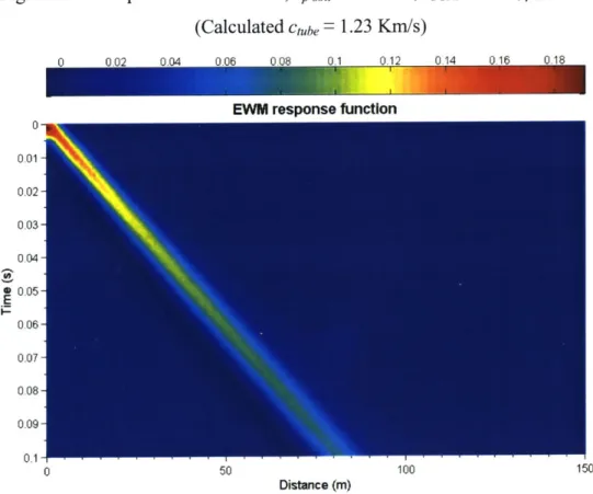
This excitation can only produce the "zero" axisymmetric mode in the pipe and so the initial pulse gets transmitted without any noise. However, since this pulse is made up from sinusoidal forms of higher frequencies as well, which attenuate faster, it gets dispersed while traveling in the pipe and it seems to extend in duration, as it can be shown by the next graphs. The graphs show the response function (product of the transfer function and the force FFT), the normalized pressure response in space and time and the pressure response at selected points in the pipe (at approximately 0, 18m, 38m and 75m from source).

(32)

Acoustical wave propagation in buried water-filled pipes Chapter 4: Simplified analysis of water filled pipe Response function 150- 100-E 50-0 0 100 200 300 400 500 600 700 800 Frequency (Hz) Figure 4.1: n I Response function (5ms 0.3 0.4 0.5 pulse) n R 07 Pressure Response 0 0.01 0.02 0.03 0.04 01 0 50 100 Distance (m)

Figure 4.2: Pressure response (5ms pulse)

Page 32 E

P-150

(33)

06

R0.4 .. . .

U') _

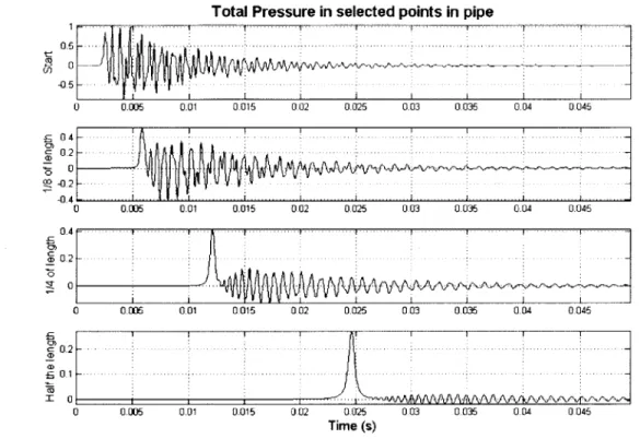
Pressure in selected points in pipe

-.-.-.-.- - - - - . . -. ...-.-.-.-. -. ... ........ ....-.-.-. ..-.-.-. ................ ....- . -0 001 002 003 004 005 006 007 008 009 22 0 2. . . . .. . . .. . . . . I .. . . .. . . .. . . 0 0.01 0.02 0.0 O.4 0.0 0.0 0.07 0.0 0.0 0 .2 -. -. -. -. -. .. - - ... . - - .- ... 0 0.01 0.02 0-0 0.4 0.0 06 0.07 0.8 0 0,6 0 .2 -. -. --. -. -. -. -. -. -. ...- .--- . ... .. ..- -- ..-- ..-- ..-.- 0 001 002 003 0.04 005 006 007 0.08 009 Time (s)

Figure 4.3: Pressure response in selected points in pipe (5ms pulse)

The above graphs show that the theoretically expected behavior is well reproduced. Figure

4.2 shows that the wave travels with a speed of 1.5Km/s (the speed of sound in water) and

that only the "zero" mode is excited in the pulse. At the same time, in figure 4.3 (but also in

figure 4.2) one can notice the slight dispersion of the wave's higher frequencies that result

in the extension of the initial pulse and the smoothening out of the pulse's starting and

ending regions. Although the initial pulse has a duration of 5ms, after 75m of propagation it lengthens up to 15ms, as it can be seen in the last part of figure 4.3.

High frequency excitations (0.2,0.5,1,2 ms puLses)

The following graphs show the response function (product of the transfer function and the force FFT), the response in space and time and the normalized pressure response at selected

(34)

Acoustical wave propagation in buried water-filled pipes Chapter 4: Simplified analysis of water filled pipe 1 2 3 4 5 6 Response function 150 100 50 0 0 0.2 0 4 0.6 0.8 1 1.2 1.4 1.6 1.8 2 Frequency (Hz) x10

Figure 4.4: Response function (0.2ms pulse)

-0.08 -0.06 -0.04 -0.02 0 0.02 0.04 0.06 0.08 Pressure Response 0 0.01 0.02 0.03 0.04 E 05 0.06 0.07 0.08 0.09 0.1 0 50 100 150 Distance (m)

Figure 4.5: Pressure response (0.2ms pulse)

(35)

. .. . . . ..

0

0 0.01 0.02 0.03 0.04 0.05 006 0.07 0.08 0.09

0.2 - - - -- - - - . - - - -...

a ooi1 0 02 oo03 0 04 0.05 0.06 0 07 oo oos.0

0-i I . . - t 7 0 0.01 0.02 0.03 0.04 0.05 0.06 0.07 0.0 0.09 0,5. ... ... . . .... 4 0 .1 00 .3 OG .0 .6 00 .8 00 0 001 0.02 0.03 0.04 0.05 0.06 0.07 0.08 0.09 Time (s)

Figure 4.6: Pressure response in selected points in pipe (0.2ms pulse)

1 2 3 4 5 6 7 8

Response function

0 1000 2000 3000 4000

Frequency (Hz)

5000 6000 7000 8000

Figure 4.7: Response function (0.5ms pulse)

I= 0 0.04 -... . .. I .2I) - -150 100 E 5 50 0 - --- --- ---- --- - ---6 --. - - ...- -. -. -.-. ...

.-.--.. ...-.--....-

- ...

-..

.

...

(36)

Acoustical wave propagation in buried water-filled pipes Chapter 4: Simplified analysis of water filled pipe 0.1 Pressure Response 0 0.01 02 0D03 0.04 S0.05 0.06 0.07 0.08 0.09 0 1 0 50 100 Distance (m) 150

Figure 4.7: Pressure response (0.5ms pulse)

05 - ---0 0 001 002 003 004 005 006 007 008 0.09 0 0 0.01 0.02 003 0.04 005 0.06 0.07 0.08 0.09 0 2 ... ... .. .. ... ... ... ... ... ... 0 -0 0.01 0.02 0.03 0.04 0.05 0.06 0.07 .O0B 0.09 a 0.5 -0 -- -1 - - -0.01 0.02 0.03 0.04 0.05 0.06 0.07 0.06 0.09 Time (s)

Figure 4.9: Pressure response in selected points in pipe (0.5ms pulse)

Page 36 0 ci) 04 0 0 Co 0 1~ 04

1~

(37)

Acoustical wave propagation in buried water-filled pipes Chapter 4: Simplified analysis of water filled pipe Response function 150 100 E 50 0 0 500 1000 1500 2000 2500 3000 3500 4000 Frequency (Hz)

4.10: Response function (1 ms pulse)

-0.2 -0.1 0 0.1 0.2 0.3 0.4 Pressure Response 0 0.01 0.02 0.03 0.04 0.05 0.06 0.07 0.08 0.09 0 50 100 Distance (m)

Figure 4.11: Pressure response (Ims pulse)

E

I-150

(38)

0 .5 - --- ...-. -.-. -. -. -. -. .....-. --. .. I . ... .. . .-. 0 0 0.01 0.02 003 0.04 0.05 0.0 007 0.08 0.09 0.. .. ... . . W . . . . . ~0.4 .- - - -- - --0 0 ₀_.01 _0.02 _0.03 _0.04 _0.05 _0.08 0.07 0.08 0.09 ! .. .. ... . . .. . . . 0 -0 2 ---- - - -0I CU T_ 0 0.01 0.02 0.03 0 04 0.06 0.06 0.07 008 0.09 0 .2 - - -. -..- -..--.. 1 0 .1 .. . ... .. .. .. .. .. .. ... .. ... .... ... .... . . .... .. .

1.

0.-0 0.01 0.02 003 0.04 005 0.06 0.07 0.08 0.09 Time (s)

Figure 4.12: Pressure response in selected points in pipe (Ims pulse)

2 Response function 150 100 50 200 400 600 800 1000 1200 Frequency (Hz) 1400 1600 1800 2000

4.13: Response function (2ms pulse)

Page 38 -. .

-0 0 __ - ____ - - - I __ I - - - - - - m - ; T__ I nifflw, - 1 -121, . ...

(39)

Acoustical wave propagation in buried water-filled pipes Chapter 4: Simplified analysis of water filled pipe 0 0.01 0.02 0.03 0.04 0 0.05 0.06 007 0.08 0.09 0.1 0.1 0.2 0.3 04 0.5 0.6 0.7 Pressure Response 0 50 100 Distance (m)

Figure 4.14: Pressure response (2ms pulse)

Pressure In selected points in pipe

0 6 - -- -- - - -. ---. 0 4 .- .-.- .-- . . -02 0 0 6 -- - - - -- - - - - -0 4

I

- -- - - - -- - -- - - - - -- -.-.-02 - - -- -- --- --0 0 0.01 0.02 0.03 0.04 0.05 0.06 0.07 0.08 0.09 150 0.01 0.02 003 0-04 0.05 Time (s) 0.06 0.07 0.08 0.09

Figure 4.15: Pressure response in selected points in pipe (2ms pulse)

0 0.01 0.02 003 004 0.6 o a 007 0.08 0.09 0 0.01 002 003 0.04 005 006 0.07 0.08 0.09 0 . 0 ~. .... . . . . ... --- - - I - --I ----.. .. .. -.. ...- . ...*. ... . .... .... .... ... . -... -... -... -... _.-... -..._. - - --...- ... -. ...- ... -- ..- .... . ... .-- - --- - -- - ... ... ... .. ... ..I-

(40)

-Acoustical wave propagation in buried water-filled pipes Chapter 4: Simplified analysis of water filled pipe

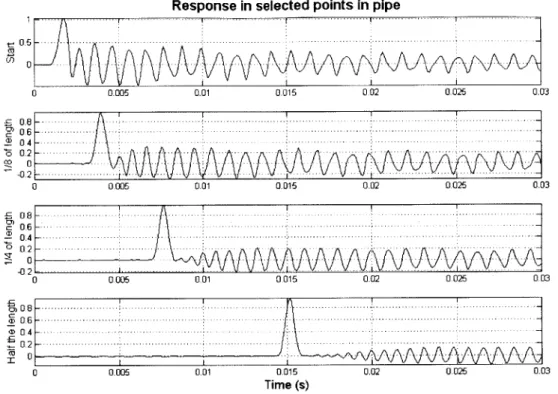
In the above graphs one can see the following major properties of high frequency wave propagation in the rigid pipe:

" The noise level increases with the increase of the frequency, but decreases very fast

with the distance the wave has traveled from the source. One can notice that, although the reverberations caused by pulses shorter than 1ms are very strong (sometimes stronger than the actual signal), at a distance of 75m the noise level is well below the main signal strength.

* The strength of the main signal decreases with an increase in the signal frequency,

since significant part of the energy of the signal is carried by the higher modes. However, as already noted, these modes attenuate much faster and so the final signal remaining has a lesser amplitude when the frequency of the excitation is higher.

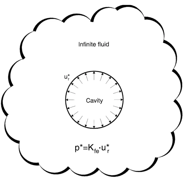
* Initially, the noise seems to travel at a very high speed and later on, as it approaches

the main signal, it shifts to the expected speed. This happens because, at start, it travels as a spherical wave, reaching the boundary of the pipe at close distances very fast. However, when the wave dominates all the cross-sectional area of the pipe it travels as a wave front with the acoustic wave velocity of the water.

* As in the low frequency case, the signal's duration seems to extend and the signal

smoothens out due to the attenuation of the higher modes.

In general, after a certain propagation distance, one expects to find no or very low noise and a signal with an extended duration which resembles the original one, having a lesser strength due to the attenuation of the "zero" mode, but mainly due to the loss of energy to the higher modes, which will have died out by that point. Consequently, at large enough distances the signal will come out clear, but one must be prepared to receive a fainter pulse than the one sent. A possible solution to long distance communication in the pipe would then be to use a very strong pulse, which will be cleared out and still have high enough

amplitude.

(41)

4.4 Conclusions

In chapter 4 a simplified analysis of the pipe was carried out to show the expected response of the system when the pipe has a much higher stiffness than the water it contains. The modes and characteristic frequencies were computed from the analytical solution and conclusions were drawn on the modes propagating in the pipe under a given frequency of excitation. The noise level was also associated with the frequency content of the excitation and the pressure-time relationship was calculated in many points inside the pipe. Moreover, it was concluded that, even for very high frequencies, the noise dies out after propagating a relatively small distance (75m maximum) compared to the propagation distance of the

main signal. As a final remark, due to the high frequency content of the noise, the signal was proven to sustain its strength much more than the noise following it, so any receiver placed downstream or upstream at an adequate distance will be certain to receive a clear

(42)

(43)

5. Beam Forming

As proven analytically and shown in Chapter 4.3, it is impossible to emit a sound signal of high enough frequency without having it spread in time and losing its strength due to its propagation. Nonetheless, high frequencies enable information transmission much faster and the success of the method of transmission lies upon this fact. So, it is easily understood that a noise reduction method is very valuable in this case. Although a lot of sophisticated filters from the branch of signal processing do exist, there is a much easier and cheaper method of noise filtering that is called "beam forming".

"Beam forming" is the alignment of sound signals in space and time so that the random noise in the conjoined received signal cancels out, while the coherent part is strengthened. In this chapter the analytical background for beam forming will be discussed and at the same time some practical uses of beam forming will be modeled. After these analyses it will be proven that the use of beam forming against noise reduction will allow for higher frequencies to be emitted and so for much more information to be channeled in the same amount of time.

5.2 Analytical considerations

In this chapter it will be shown that the analytical manipulation of the transfer function that describes the pressures in the pipe (or any attribute of the response for that matter) in the time and space domain is of no practical use and therefore there is no way to analytically calculate the joint response of the two sources. However, after understanding the noise problem in the pipe, it is relatively straightforward to position the sources' excitation in space and time to achieve the required noise reduction.

(44)

The analytical calculation of the beam forming response, based on the response of a single source, is not trivial. This is due to the inverse Fourier transformation, which the data must go under, and the summation of the different terms of the series as follows:

If the second source is spaced zo away from the first one and "fires" at to after the first one the transfer function of the pressures inside the pipe will have the form of:

--i(z-z0) k -ki;

p'(r, 0, z, ca)= 2 o f (o)e e 2 (given that the pressure is

j=1 Jkk (k0.R)

calculated at the center of the pipe, r=O)

It is easy to see that the exponential term of e- -kSi has a different value for each term

and therefore cannot be factorized and used outside the Fourier integral. At the same time

the e-'itO term, although equal for all

j,

cannot be factorized out of the Fourier integral,

because it contains the integration variable co. Consequently, there is not easy to derive formula that simulates the response of the system under the beam forming loading.

However, knowing the response function of the system and observing its maximum value region, one can get a fairly good estimation of a relationship between the delay and the spacing of the second source. Given that these must be linked through a wave speed of approximately 1.5 Km/s, one can then calculate the required zo and Ato. The following chapter will show how this can be done, given the dimension of the pipe and the signal properties.

5.3 Practical uses

Assuming a pipe of im radius under different kinds of excitation, this chapter will demonstrate how to space apart the second source and the delay required for a substantial noise reduction. The excitations used will be of high frequency content, so that they can generate enough noise. The term "intermediate noise level" is used to signify noise that has maximum amplitude equal to the initial signal strength, while the "high noise level" refers to noise that can exceed the initial signal in amplitude. The results will show the difference

Page 44

(45)

between the response of the system to a single source loading and a beam forming with 2 sources.

1 ms pulse (intermediate noise level)

This pulse will have a response function (for the single source) as shown in the next graph:

0.5 1 1.5 2 2.5 Response function 150 100 0I 50 0 500 1000 1500 2000 2500 3000 3500 4000 Frequency (Hz)