HAL Id: hal-01859899
https://hal.archives-ouvertes.fr/hal-01859899
Submitted on 22 Aug 2018
HAL is a multi-disciplinary open access
archive for the deposit and dissemination of
sci-entific research documents, whether they are
pub-lished or not. The documents may come from
teaching and research institutions in France or
abroad, or from public or private research centers.
L’archive ouverte pluridisciplinaire HAL, est
destinée au dépôt et à la diffusion de documents
scientifiques de niveau recherche, publiés ou non,
émanant des établissements d’enseignement et de
recherche français ou étrangers, des laboratoires
publics ou privés.
Inductance and Frequency-Dependent Resistance of
Windings in Transformers
Alexis Fouineau, Marie-Ange Raulet, Bruno Lefebvre, Noël Burais, Fabien
Sixdenier
To cite this version:
Alexis Fouineau, Marie-Ange Raulet, Bruno Lefebvre, Noël Burais, Fabien Sixdenier. Semi-Analytical
Methods for Calculation of Leakage Inductance and Frequency-Dependent Resistance of Windings
in Transformers. IEEE Transactions on Magnetics, Institute of Electrical and Electronics Engineers,
2018, 54 (10), pp.8400510. �10.1109/TMAG.2018.2858743�. �hal-01859899�
0018-9464 © 2015 IEEE. Personal use is permitted, but republication/redistribution requires IEEE permission. See http://www.ieee.org/publications_standards/publications/rights/index.html for more information. (Inserted by IEEE.)
Semi-analytical methods for calculation of leakage inductance and
frequency-dependent resistance of windings in transformers
Alexis Fouineau
1,2, Marie-Ange Raulet
2, Bruno Lefebvre
1, Noël Burais
2and Fabien Sixdenier
21SuperGrid Institute, Villeurbanne, France
2Univ Lyon, UCB Lyon 1, CNRS, AMPERE, Villeurbanne, F-69100, France
Leakage inductance and frequency-dependent resistance of windings are key parameters for the design of magnetic devices. This report focuses on analytical or semi-analytical calculation techniques to be integrated into a medium frequency transformer optimization process. To this extend, a review of currently most used method to calculate inductance and resistance of windings transformer is established. Based on this review, new calculation methods are developed. Magnetic field cartography is evaluated on the basis of two-dimensional structures thanks to a combination of Ampère’s law and image method. From this magnetic field map, leakage inductance can be calculated. The obtained accuracy with this method is equivalent to three-dimensional finite element modeling. For frequency-dependent resistance evaluation, new methods based on two-dimensional or one-dimensional approach are compared to finite element modeling and reviewed models. An analysis of behavior of each model is done, showing that newly developed models are more suitable in the case of medium frequency transformer design in terms of accuracy, robustness and calculation time. This work could be useful to magnetic devices designers because newly developed models could easily be adapted to various geometries, such as toroidal structures or even inductors.
Index Terms— Eddy currents, Electric resistance, Inductance, Power transformers
I. INTRODUCTION
In the field of energy conversion, power electronics will play a major role. For example, the use of solid-state transformers can provide new solutions to future electrical grids and traction networks [1]. It allows better connection of new renewable energy source such as far offshore wind farms [2]-[3], or reduction of energy consumption for traction systems thanks to higher efficiency and lower weight [4].
A key component of solid-state transformers is the medium frequency transformer, typically operating between 500 Hz and 20 kHz to reduce its size. Its main role is to provide a galvanic insulation but the converter also takes advantage of other intrinsic properties of transformers: transformation ratio, magnetizing and leakage inductances. The design of medium frequency transformer must take into account all these specifications, which involves a multi-objective optimization process [5]-[6].
In this paper, we will focus on a crucial active part of the medium frequency transformers which is the windings. Two windings characteristics must be evaluated accurately during the design process: AC resistance and leakage inductance [7].
The design process usually need low calculation time models to allow a great number of calculation points in the shortest time possible. Therefore, most of the accurate numerical solutions, such as finite element modeling (FEM), leading to high calculation time are not suitable. Analytical or semi-analytical models are usually better solutions.
The purpose of this paper is to propose new models to calculate leakage inductance (considering steady current) and frequency-dependent resistance of windings and to compare them with existing ones. To this aim, part II will present existing and newly developed calculation methods for both inductance and resistance. Then, part III will evaluate all previously identified models on typical test cases. The
accuracy and calculation time results given by the various models will be presented, and compared to numerical FEM calculation results in part III. Finally, part IV will analyze the performances of the different calculation methods and will list advantages, disadvantages and limitations of each one.
II. METHODS
In the case of medium frequency applications, it is important to note that the same magnetic fields are responsible for both stored energy and eddy currents, i.e. leakage inductance and frequency-dependent resistance. It is the reason why the calculation of magnetic field is a prerequisite.
A. Magnetic fields and leakage inductance 1) One-dimensional field of concentric windings
A classical geometry of transformer is the case of concentric primary and secondary windings inside a winding window as shown in Fig. 1.
Fig. 1. Concentric windings inside a winding window and associated one-dimensional magnetic field distribution.
In this case, the magnetic field H is oriented along the winding axis y. The maximal value of H is located between the windings, and can be calculated thanks to Ampère’s law. The expression is shown in (1), where I is the total magnetomotive force and h is the windings’ height. Finally,
H increases and decreases linearly in both windings.
y y
e
H
H
H
max
I
/
h
(1)This calculation method is widely used in transformer design because of its simplicity, but its limitations should not be forgotten. This model does not work if there is not a complete Ampère-Turns compensation between primary and secondary, such as in the case of an inductor. If the windings are not confined into a winding window or even if the winding height is inferior to the winding window height, then one-dimensional field hypothesis becomes false. This is why a two-dimensional approach might become necessary.
2) Field of basic conductors
This paragraph explains how to calculate magnetic field produced by a single conductor carrying a current inside vacuum. Two basic shapes of conductor will be considered: round and rectangular. These basic conductors will be used extensively for magnetic field two-dimensional calculation in transformers.
a) Round conductor
A round conductor of radius rc carrying a current I is
considered. Magnetic field in this case is purely orthoradial and its expression inside and outside the conductor can be easily obtained from Ampère’s law (2).
) 2 /( ) 2 /( ) ( 2 r I H r rI H c if if c c r r r r (2)
Fig. 2 shows a schematic of the configuration as well as an example of magnetic field cartography in this case.
Fig. 2. Schematic of a round conductor and magnetic field distribution of a 1 mm radius conductor carrying 1 A.
b) Rectangular conductor
In the case of a rectangular conductor, H is not orthoradial, particularly inside and near the conductor. However, its component can be calculated by using (3) (development may be found in [8]).
1 2 1 2 1 1 1 2 1 1 2 2 2 1 2 1 log log 8 log log 8 r r b y b y a x a x ab I H r a x r a x b y b y ab I H y x (3)Fig. 3 shows a schematic of the configuration with all the parameters mentioned in (3), as well as an example of magnetic field cartography in this case.
Fig. 3. Schematic of a rectangular conductor and magnetic field distribution of a 1 mm 2 mm conductor carrying 1 A.
3) Conductors next to a column
In this configuration, one or several basic conductors are considered placed next to a column constituted of a high permeability material, the conductors themselves being in vacuum. This configuration might be representative of the case where the concentric windings are outside the winding window.
Using magnetic image method [9], this situation is equivalent to having mirrored conductors as shown in Fig. 4. The schematic is just here to illustrate how the magnetic field can be calculated for any shape of conductors next to a magnetic circuit.
Fig. 4. Image method for conductors next to a high permeability material surface.
Usually, transformer core material has a very high permeability with µr > 1000. But if not, equation (4) can be
used to set the value of currents in image conductors.
I I r r image 1 1 (4)
The problem is then equivalent to multiple conductors in vacuum, and superposition principle can be used to determine total magnetic field as shown in (5).
c c
conductor
c c
conductorx y H x y
H
H , , (5)
A similar approach has been developed in [10], by using Biot-Savart law and discretization of the windings in multiple source points. Both methods are equivalent, but the one developed here requires less discretization and should be easier to implement. Nevertheless, windings sections must be a combination of round and rectangular shapes for the method presented here (5) to be applicable.
4) Conductors inside a winding window
One-dimensional field assumption is not always valid inside a winding window, for example when windings heights are not the same or do not match the window height, which is often the case for power transformers. This is why a two-dimensional magnetic field calculation might be necessary.
Applying the image method to conductors inside a winding window would theoretically create an infinity of image conductors. This is because the mirror effect of image method not only duplicates the current sources, but also the material interfaces [11]. It creates mirrored version of magnetic mirrors. For a winding window, there are two pairs of magnetic mirrors which results in a sort of infinite tiling of the two-dimensional space as shown in Fig. 5. Mirrored cells may be indexed with m and n depending on their position relative to the original cell. A and B are respectively the winding window width and height.
Fig. 5. Image method for conductors inside a winding window.
Nevertheless, superposition principle remains valid even for an infinity of conductors and total magnetic field may be calculated with (6), where the position of image conductor according to cell index is obtained from (7) considering geometric parameters defined in Fig. 5.
m n conductoram b n H H , (6) odd is if , even is if , ) ( odd is if , even is if , ) ( n b B nB n b nB n b m a A mA m a mA m a (7)However, it is not possible numerically to compute the magnetic field of the theoretical infinity of cables. Therefore, in practice, a limited number of cells must be considered. From (2) and (3), it is clear that an image conductor far away from the original cell will have a low contribution to magnetic field value inside the original cell. In practice, setting an empirical limit such that only reflected conductors distant less than the maximal dimension of A and B from the original cell must be taken into account gives good results.
A similar approach has been established in [11]. However, a preferential direction was supposed to take into account the infinity of conductors. This last assumption was too restrictive and consequently the calculated field was highly inaccurate in certain zones of the window area.
5) Core-type and shell-type leakage inductance
The previous models for calculation of two-dimensional magnetic field can now be applied to some transformer structures.
In particular, core-type and shell-type structures, which are the most common ones for power transformers, can be studied with a multiple 2D planes analysis. As shown in Fig. 6, each plane represents a portion of the geometry of the transformer and has its associated depth. The planes numbered “1” correspond to conductors inside the winding window, and the planes numbered “2” correspond to conductors next to a column but outside the winding window.
Fig. 6. a) Core-type structure. b) Planes and associated depths for core-type structure (top view). c) Shell-type structure. d) Planes and associated depths for shell-type structure (top-view).
Determining the total leakage inductance of a transformer can be carried out by setting perfectly opposed magnetomotive forces into the primary and secondary windings and
calculating the total magnetic energy Emag. This energy will
then correspond only to leakage flux because magnetizing flux will be equal to zero. To calculate this energy,firstly magnetic field is calculated for each 2D plane. Then this field is integrated over the whole plane to get the value of the plane energy E2D. This integration must be performed over a
sufficiently large area for infinite or semi-infinite configurations (winding next to a column). Any numerical integration method is possible as long as a good precision and a low calculation time are guaranteed. Finally, the energies
E2D are multiplied by their respective depths d2D and summed
using (8) to obtain the total magnetic energy Emag.
D D
mag E d
E 2 2 (8)
Leakage inductance can then be obtained from (9), where I is either primary or secondary current depending on which side the leakage inductance is considered.
2 2 1 LI Emag (9) B. Frequency-dependent resistance
At low frequency or direct current, winding resistance can be simply calculated from material electrical conductivity and geometric dimensions. However, when the frequency increases, magnetic field will create eddy currents in opposition to excitation current due to Faraday’s law of induction.
These eddy currents can be categorized into two types representing skin effect and proximity effect [12]. Skin effect corresponds to eddy currents inside a conductor created by the current flowing in the same conductor. Proximity effect represents eddy currents inside a conductor created by currents flowing in nearby conductors. Because both phenomena originate from two independent sources, they are independent [13]. Total losses can be split as shown in (10), where I is the peak current inside the conductor, Hext is the magnetic field
produced by nearby conductors and f is the frequency.
I P
I f
P
H f
P
PJoule DC skin , prox ext, (10)
A practical way to represent the increase of losses with the frequency is to use factors quantifying this increase compared to DC losses. In this paper, skin factor defined in (11) and proximity factor defined in (12) will be used.
1 DC skin DC S P P P F (11) 0 DC prox P P P F (12)
It should be noted that skin effect losses Pskin are directly
related to the current I flowing inside the considered conductor
and this is why it makes sense to define skin factor in (11). However, proximity effect losses Pprox are indirectly related to
the current I. In fact, proximity losses are due to the external magnetic field Hext. But in transformer windings, external
magnetic field Hext is a function of the current I. This function
depends on the transformer geometry (number of turns, number of independent conductors per turns and location of each independent conductor). So it also makes sense to define a proximity factor in (12).
Finally, the frequency dependent resistance RAC and the
global resistance factor FR are defined thanks to (13).
S P
DC DCR
AC FR F F R
R (13)
These factors will be used to consistently define the different models. Next paragraphs will present various existing models and the development of new ones.
1) Dowell’s model
Dowell’s model [14] is probably the most commonly used one to calculate frequency-dependent resistance in transformer design phase. Main hypothesis of this model is the one-dimensional magnetic field, as presented previously in II.A.1. Windings are supposed to be composed of m successive layers of thickness d parallel to the magnetic field. By definition, these layers must have a rectangular shape, which is very suitable for windings constituted of foil or flat conductors.
However, in the case of round wires cables or Litz cables, this model can be adapted by the introduction of a porosity factor ηw (ratio of winding height hw and window height h).
Round conductors are transformed to square ones and empty space between them is taken into account through the porosity factor. In the following equations, δ represents the skin depth at the considered frequency.
h δ πf h d d X w w 1 ' (14)
2 '
cos
2 '
cosh ' 2 sin ' 2 sinh ' X X X X X FS (15)
' cos ' cosh ' sin ' sinh ' 1 3 2 2 X X X X X m FP (16) 2) Ferreira’s modelThis model also considers the case of a one-dimensional field, but unlike Dowell’s model, basic conductors are supposed round [15]. In the following equations, ds is the
diameter of a basic conductor (strand or wire), and bern and bein are the Kelvin-Bessel functions of order n.
2
2 2 ' ' ' ' 2 ber bei ber bei bei ber FS (18)
P P P P K f m f F 2 12 (19)
2 2' 22 ' bei ber ber bei bei ber fP (20)Proximity factor has been factorized into two terms in (19).
KP represents the winding structure factor and is independent
of the frequency, whereas fP represents the
frequency-dependent factor and depends only on frequency and conductor diameter.
3) Reatti and Kazimierczuk model
In [16], the authors have developed a model very similar to Ferreira’s one. However, the porosity factor has been taken into account. All formulas are the same as Ferreira’s model except for the winding structure factor defined by (21).
1 3 1 4 2 2 m KP w (21)Other models based on Ferreira’s model exist, considering various structures for windings. For example, Litz cable structure is considered in [17] and [18]. However, main hypotheses (one-dimensional field and layers inside winding) are the same therefore these models will not be considered in this paper.
4) Asymptotic model
Contrary to previously presented models, this one does not take into account skin effect and only represents impact of proximity losses due to external magnetic field. Therefore
FS = 1 and FR = 1 + FP.
The basic formula is presented in [19], and expresses the proximity losses inside a round conductor of diameter ds
inside a homogeneous magnetic field H as shown in (22). In this equation, ρ is the resistivity, µ the permeability, l the length and ω the angular frequency.
128 2 2 4 2ld H P s prox (22)
For a winding of width w, height h containing N turns placed inside a one-dimensional field such as the one described in II.A.1, a proximity factor can be expressed as shown in (23). Development of this equation may be found in Appendix A, and η corresponds to the proportion of conductive material inside the winding being considered as composed of evenly distributed round conductors with insulating material between them.
h Nw f d F s P 2 2 4 2 3 48 (23)
For a given geometry, the proximity factor is proportional to f 2. Thus it creates a line in logarithmic scale and this is why
this model is called “asymptotic”.
5) Albach’s model
In [20], the author has developed formulas for both skin and proximity losses inside a round conductor subject to any external magnetic field distribution.
Skin factor is expressed as shown in (25) where α is defined in (24). In is the modified Bessel function of first kind and a is
the radius of the conductor.
1i (24)
a I a I a FS 1 0 Re 2 1 (25)Proximity losses are calculated thanks to spatial Fourier series decomposition. In (26), coefficients ak and bk (resp. ck
and dk) are the decomposition coefficients of Hr (resp. Hφ) on
the surface of the conductor in polar coordinates.
II aa a d a c b l P k k k k k k k prox 1 1 2 2 Re 2 (26)However, windings composed of Litz wires have strands whose size is usually very small compared to the size of the winding itself. Therefore external magnetic field can be considered constant over a strand. In this case, previous equation can be simplified into (27) as shown in Appendix B.
a I a I a H l Pprox 0 1 2 Re 2 (27)Finally, a proximity factor can be expressed under the assumption of a one-dimensional field with the same method used for asymptotic model, as shown in (28). The development of this equation may be found in Appendix A.
a I a I a h Nw f K FP P P 0 1 Re 3 4 (28)This proximity factor was split into a frequency- independent factor KP and a frequency-dependent factor fP, as
done previously with Ferreira’s model. In fact, Albach and Ferreira models have the same skin factors FS and
frequency-dependent factor fP (demonstration in Appendix C); the only
difference between them lies in the expression of the winding structure factor KP.
III. RESULTS
A. Magnetic fields and leakage inductance
To test out the models of magnetic field and leakage inductance calculation, structures presented on Fig. 6 were used. The considered geometry has a winding window of 100 mm 200 mm. Windings are 150 mm high, the distance between the first winding and the core is 10 mm, and the distance between the second winding the and first winding is 20 mm. Both windings are comprised of only one turn for the purpose of calculation. For both core-type and shell-type structures, the same geometry is used but the winding window of the core-type structure contains a total of four windings whereas the shell-type one has only two windings.
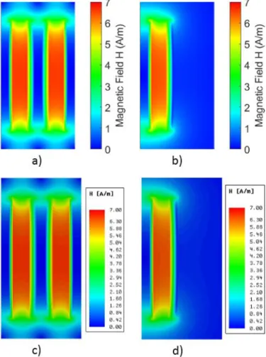
Fig. 7 shows the magnetic field obtained for the core-type structure inside and outside the winding window, with a current of 1 A flowing inside each winding. Magnetic fields obtained with 2DFEM or with analytical model look identical. To confirm this observation, total energies of these planes were calculated and compared in Table I. The maximum difference on the calculation results between the two different methods is below 1%.
Fig. 7. Magnetic field distribution for: a) Winding window, analytical model; b) Leg side, analytical model; c) Winding window, 2DFEM; d) Leg side, 2DFEM.
From these energy values, total leakage inductance was calculated analytically on each structure. Also, the newly developed “2x2D” model was compared to classical 1D method using magnetic field calculated as presented in II.A.1 on the one hand, and to 3DFEM results on the other hand. This comparison is available in Table II. The “2x2D” method gives results very close to 3DFEM ones with less than 2% deviation, whereas one-dimensional approach overestimates leakage inductance by more than 10% in this case.
B. Frequency-dependent resistance
To be able to compare the calculation results achieved by the analytical models and the 2D finite element modeling, a typical transformer structure was considered. This two-dimensional structure is located inside a winding window and constituted of two identical windings. Basic conductors are strands with 0.5 mm diameter and 33 µm enamel thickness. A winding is made up of 1 000 strands organized as shown in Fig. 8, with 10 strands per horizontal row. Horizontal distances between core and windings and between windings are all equal to 5 mm. Finally, the winding height wh is equal
to 56.6 mm and the vertical gap eh is fixed to obtain the
desired porosity factor following (29) where Ds and ds are the
strand diameter with and without enamel.
h h h s s w e w w D d 2 4 (29) TABLEI
COMPARISON OF MAGNETIC ENERGY OF PLANES
Plane Energy (Analytical) Energy (FEM) Difference Winding window 1.8885.10-7 J/m 1.8963.10-7 J/m -0.41% Led Side 9.0958.10-7 J/m 9.0944.10-7 J/m +0.01%
Comparison of energies of considered planes obtained with analytical method and with finite element method (FEM) simulation. FEM is considered as reference.
TABLEII
COMPARISON OF LEAKAGE INDUCTANCE CALCULATION METHODS
Structure Method Leakage
Inductance Difference Time
Core -type Analytical 1D 1.6775.10-7 H +13.44% 0.3 ms Analytical 22D 1.4691.10-7 H -0.54% 230 ms FEM 3D 8k tetrahedrons 1.4896.10-7 H +0.85% 28 s FEM 3D 1M tet. 1.4770.10-7 H 0% 3066 s Shell -type Analytical 1D 8.3776.10-8 H +13.84% 0.3 ms Analytical 22D 7.2434.10-8 H -1.57% 100 ms FEM 3D 5k tet. 7.4310.10-8 H +0.98% 21 s FEM 3D 0.7M tet. 7.3590.10-8 H 0% 1139 s
Comparison of leakage inductance values obtained with analytical and numerical methods. FEM 3D with 0.7 - 1 million tetrahedrons is taken as reference.
Fig. 8. Geometry definition of windings and window used for test cases of frequency-dependent resistance calculation.
Even if this geometry may not be representative of a Litz wire winding of a medium frequency transformer, it is a good test case to compare models with each other. Moreover, the limited number of strands allows a good meshing of the geometry for finite element modeling by using an eddy current solver (in this case, ten triangles along a strand diameter) with reasonable computation time. It should be noted that in this configuration, current was considered equally divided between all strands, which corresponds to an ideal twisting pattern. Fig. 9 presents the obtained results in all considered cases of porosity factors. The resistance factor was calculated with each of the models and FEM modeling for various frequencies (corresponding to ratio diameter to skin depth ds/δ) in the
range of 100 Hz - 1 MHz. For asymptotic and Albach, 2D refers to (22) and (27) being used with a two-dimensional magnetic field calculation method, whereas 1D refers to (23) and (28).
From these results, Dowell’s model is always closer to FEM one than Ferreira’s or Reatti’s. Moreover, asymptotic model gives the same results as Albach’s one at low frequencies whereas it is completely false at higher frequencies. Therefore, Dowell and Albach look as the best performing models.
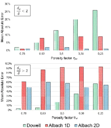
To compare them in a better way, two main zones can be considered: before and after a ratio of diameter to skin depth of 2. The mean absolute error was calculated for each model in both zones and results are presented in Fig. 10. Dowell’s model presents an error increasing consistently with the reduction of porosity factor in each zone. However, Albach’s model has an error quite independent of the porosity factor. This error remains low at low frequencies, particularly for Albach 2D, but it is much higher at high frequencies.
To complement these results, it should be mentioned that the calculation time is about 0.5 ms for all one-dimensional models and about 25 ms in the case of two-dimensional models.
Fig. 9. Frequency-dependent resistance factor obtained for all tested models on test cases with different porosity factor (one per graph).
Fig. 10. Mean Absolute Error (MAE) of three best-performing models. First graph is MAE only for frequencies where skin effect is negligible. Second graph is MAE only for frequencies where skin effect is not negligible.
IV. DISCUSSION
A. Magnetic fields and leakage inductance
For magnetic field calculation, results show very good agreement between the newly developed “2x2D” method and 2D finite element modeling. Magnetic fields and plane energies are almost identical in the considered case.
Moreover, leakage inductance calculation based on this “2x2D” method presents a good accuracy when comparing with finite element modeling for both core-type and shell-type structures. It means that the decomposition of the structure in multiple characteristic planes is a good hypothesis.
However, the accuracy of this approach is limited inside the winding window because the calculation would require an infinity of images to make the error close to zero. This limitation is highlighted by a small difference of 0.41% between numerical simulation and plane energy in Table I, whereas leg side results are almost identical with a difference of 0.01%.
Winding window energy is not the only cause of difference between leakage inductance calculated analytically and numerically. The other one is the two-dimensional decomposition. In fact, the associated depth of each plane is inaccurate because the geometry varies along this depth, particularly in corner region of windings as it can be seen on Fig. 6. It explains why there is more difference for leakage inductance than for planes energies. Nevertheless, accuracy (below 2%) can be considered as very satisfying, especially when considering that calculation time has been reduced by
more than 100 times. However, one-dimensional calculation is still faster because there is no discretization at all, but at the expense of a much lower accuracy. So the newly developed “2x2D” model is a good compromise between accuracy and calculation time.
This model is also a very good solution to compute magnetic field only in a specific area without having to calculate it over the whole geometry, as it is the case in finite element modeling.
Finally, maybe the most important advantage of this model is its adaptability. The method used is very general and applicable to almost any transformer or magnetic device geometry, provided that it can be decomposed into multiple two-dimensional structures (symmetries). There is no need for windings to be concentric, and it can be easily adapted to toroidal structures by using the two-dimensional decomposition presented in [21].
B. Frequency-dependent resistance 1) General comments
In the case of frequency-dependent resistance calculation methods, the results show a great disparity between models on accuracy levels and frequency behavior. First of all, three main zones can be considered for resistance factor curve obtained by FEM, in black straight line on Fig. 9. First zone corresponds to a resistance factor close to one which means that there is no significant proximity or skin effect. Then, by increasing the frequency, a second zone appears with a first slope corresponding to proximity effect. This transition can occur at different ratio ds/δ depending on the geometry. Here,
the geometry of the winding does not vary so much between the different cases so the transition always occur around ds/δ =
0.7. Finally, the last zone corresponds to another slope, lower than the previous one, combining proximity and skin effects. This transition will always occur around ds/δ = 2 because of
skin effect. These three zones and their associated boundary frequencies have been identified in [22] and [23]. Actually, skin effect is already present before this limit but is not high enough to have a significant impact on the resistance factor. The slope in this zone is lower because the skin effect acts as a shielding of the strands and prevents the penetration of external magnetic field inside them, thus confining proximity effect in a reduced portion of the conductors. In other words, magnetic field induced by eddy currents is not negligible anymore in this zone and reduce drastically the static magnetic fields inside conductors.
Before discussing the results obtained for each model, it should be noted that, in the case of medium frequency transformer, the accuracy level in the zones before ds/δ = 2 is
much more important that the one obtained after. In fact, a proper design must have a low resistance factor, and this case usually corresponds to the situation where skin effect is negligible if an important number of conductors has to be considered. Therefore, the inaccuracy that can occur in the high frequency zone will mostly impact designs that wouldn’t have been retained (in a first design step) because their losses would have been too high even in the low frequency region.
However, it is still relevant to be accurate enough in this zone (after ds/δ = 2), in a second design step, for possible
high-frequency harmonics of the considered current, and ensure that these harmonics will not cause too many additional losses.
2) Models comparison
Ferreira’s model always overestimates resistance factor. This is because the porosity factor is not considered for this model and therefore the gaps between conductors are ignored as if the vertical dimension was completely filled with conductors. It results in an overestimation of proximity losses. This is why this model will not be further investigated.
Dowell’s model is almost exact for a porosity factor of 0.78. In this case, the distance between windings and core eh is zero
and the porosity factor is only due to gaps between strands inside windings. Therefore, the one-dimensional hypothesis for magnetic field is valid. The use of equivalent foil to represent strands seems to be in accordance with Dowell’s hypothesis regarding the level of accuracy obtained (less than 2%). The model remains exact even at high frequency where skin effect is important because Dowell’s model is not influenced by magnetic field of nearby conductors. In fact, the equation is obtained by setting boundary conditions on both sides of the foil and solving Maxwell equations. The field on the side of the foil is independent of the frequency so boundary conditions remain valid on the whole frequency range and the equation of the resistance factor is also valid. This is why Dowell’s model gives the best results in the case of one-dimensional field. However, when the distance between core and windings increases, one-dimensional hypothesis is no longer valid which explains why Dowell’s model accuracy decreases in both zones before and after significant skin effect.
Reatti and Kazimierczuk model is similar to Ferreira’s model except that it takes into account the porosity factor. This is why the model behaves like Dowell’s model. However, its accuracy at high frequency is limited because the eddy currents due to magnetic field induced by eddy currents of nearby conductors is not taken into account. Thus this model is less accurate than Dowell’s one and will not be further investigated.
The main disadvantage of the asymptotic model is its behavior in the high frequency zone. Even if the resistance factor is accurate at low frequency, skin effect is not considered at all. Therefore, no shielding effect is preventing eddy current development inside conductors at high frequency, and the losses are greatly overestimated. Everything happens as if proximity effect was independent of frequency, and this is why the asymptotic behavior occurs. The disadvantage is the same for one-dimensional or two-dimensional versions, so this model will not be further investigated.
For a porosity factor of 0.78, Albach’s model has the same behavior as Reatti and Kazimierczuk. This is because in this case, formulation of equations are almost equivalent. It means Albach’s model suffers from the same limitation at high frequency, not taking into account mutual influence between
conductors due to magnetic field produced by eddy currents. However, when the porosity factor decreases, Albach’s model accuracy remains almost constant. This is because the porosity factor is not directly used, but the proportion of conductive material inside winding η is considered instead. Overall, this is why this model gives the best results in the cases of low porosity factor, with a very good accuracy at low frequency and a contained error at high frequency. The one-dimensional version of the model has an error of less than 10% at low frequency and below 100% at high frequency, whereas the two-dimensional version has an error below 2% at low frequency and 60% at high frequency. In fact, both versions have the same accuracy for a porosity factor of 0.78 because one-dimensional hypothesis is valid in this case. For lower porosity factor, the two-dimensional model is logically more accurate because the magnetic field is two-dimensional. However, if calculation time is critical, the one-dimensional version is still a solution for this type of geometry.
All these observations explain why Albach’s model is considered as the best candidate for medium frequency transformer design. It provides a good accuracy and a great resilience to porosity factor variations from a design to another, with no additional calculation time in its one-dimensional version. Actually, it is even faster than Dowell’s model as Bessel functions inputs depend only on strand diameter and frequency, whereas the inputs of trigonometric functions of Dowell’s model include the porosity factor and therefore depend on the transformer geometry. This allows a reduction of the calculation time when applied to a great number of geometries.
Moreover, the model is very adaptable. As long as the magnetic field is known for a given geometry, the proximity losses can be calculated and a resistance factor formula can be derived. This hypothesis is still satisfied for configurations without concentric windings, such as toroidal structures or even inductors where there is no secondary and therefore no Ampère-Turns compensation.
Nevertheless, this model has some limitations. First one, already discussed, is its reduced accuracy at higher frequency. This problem could be limited if equation (26) was used instead of its simplified version (27) and an iterative process was followed [20]. This last option would complicate the model implementation and it would have a high negative impact on the global calculation time in a first design step. A possible way would be to use the improved version only for a very limited number of designs (second design step). It leads us to another downside of this model which is the necessity of calculating magnetic field inside windings with enough accuracy. The method presented in this article to calculate magnetic field is very adaptable, but at high frequency, the windings cannot be homogenized as a macroscopic rectangular conductor and each strand contribution must be considered. Therefore the computation time would depend on the number of strands, which is a real inconvenience. A way to solve this last problem would be to combine Albach’s model to determine equivalent complex magnetic permeability and
electrical conductivity for a given winding structure, following a method such as the one presented in [24]. It would correct the accuracy at higher frequency, but to the detriment of a more complex model and an important calculation time. This could be a solution to calculate a precise frequency-dependent resistance for specific designs, but again, it is not suitable for integration inside an optimization process.
V. CONCLUSION
In this article, a review of magnetic field, leakage inductance and frequency-dependent resistance calculation methods has been done. For each subject, new methods of calculation were developed. The two-dimensional (“2x2D”) method for magnetic field calculation revealed its accuracy with low calculation time, and leads to precise leakage inductance evaluation in the case of usual core-type and shell-type transformer structures.
Concerning the frequency-dependent resistance calculation method, the newly developed model based on Albach’s theory is more accurate, more robust and faster than reviewed models.
Overall, newly developed models are already an improvement from reviewed ones, and are very promising due to their possibility of further improvements: adaptability to new structures (toroidal, inductors) and increased accuracy for high frequency. In this sense, they are very good candidates for magnetic devices design and optimization. Implementation of these tools is in progress.
APPENDIX A
Demonstration of one-dimensional proximity factor for asymptotic model. y y e h NI w x e H w x H max
h w h w s s strand strand prox dxdy d H ld dxdy S P P 0 0 0 0 2 2 2 4 2 4 128 h w I N d l P s prox 96 2 2 2 2 2 2 2 s dc d lNI P h Nw f d P P F s DC prox P 2 2 4 2 3 48 Demonstration of one-dimensional proximity factor for Albach’s model.
h w h w s strand strand prox dxdy d a I a I a H l dxdy S P P 0 0 0 0 2 0 1 2 4 Re 2
a I a I a h d w I lN P s prox 0 1 2 2 2 Re 3 8
a I a I a h Nw P P F DC prox P 0 1 Re 3 4 APPENDIX BSimplification of Albach model in case of homogeneous magnetic field.
Series Fourier of any magnetic field in polar coordinates on the surface of the conductor:
1 1 sin cos , sin cos , k k k k k k r k d k c a H k b k a a H If magnetic field is constant over the strand:
H H
e H H
e H e H e H H x y r y x y y x x sin cos sin cos By identification: x H a1 b1Hy c1Hy d1Hx 0 k k k k b c d a for k1Then by injecting this result in (26), one can obtain (27). APPENDIX C
Demonstration of equality between FS and fP of Albach and
Ferreira models. 1i 2 ds 4 4 2 2 2 1 i i s s d e e d i a
Relations between Bessel and Kelvin-Bessel functions:
2 4 i n ni n n x i bei x e I xe ber
ber
x x n x bei x ber x ber n n n n 2 ' 1 1
bei
x x n x bei x ber x bei n n n n 2 ' 1 1
2 2 2 1 2 1 1 1 1 1 1 1 4 1 0 ' ' ' ' 2 2 2 Re 2 1 Re 2 1 bei ber ber bei bei ber bei ber bei ber bei bei ber ber bei i ber bei i ber i e a I a I a F i S Same method is applied for (20) and (28):
2 2 2 2 2 2 1 1 1 1 1 1 4 0 1 ' ' 2 Re Re bei ber ber ber bei bei bei ber bei ber ber bei ber bei bei i ber i bei i ber e a I a I a f i P ACKNOWLEDGMENTThis work was supported by a grant overseen by the French National Research Agency (ANR) as part of the “Investissements d’Avenir” Program (ANE-ITE-002-01).
REFERENCES
[1] J. W. Kolar and G. Ortiz, "Solid-state-transformers: key components of future traction and smart grid systems," in Proceedings of the
International Power Electronics Conference-ECCE Asia (IPEC 2014),
2014.
[2] A. Prasai, J.-S. Yim, D. Divan, A. Bendre and S.-K. Sul, "A new architecture for offshore wind farms," Power Electronics, IEEE
Transactions on, vol. 23, pp. 1198-1204, May 2008.
[3] T. Lagier and P. Ladoux, "A comparison of insulated DC-DC converters for HVDC off-shore wind farms," in 2015 International Conference on
Clean Electrical Power (ICCEP), 2015.
[4] D. Dujic, F. Kieferndorf, F. Canales and U. Drofenik, "Power electronic traction transformer technology," in Proceedings of The 7th
International Power Electronics and Motion Control Conference, 2012.
[5] A. Garcia-Bediaga, I. Villar, A. Rujas, L. Mir and A. Rufer, "Multiobjective optimization of medium-frequency transformers for usolated soft-switching converters using a genetic algorithm," IEEE
Transactions on Power Electronics, vol. 32, pp 2995-3006, 2016.
[6] M. Leibl, G. Ortiz and J. W. Kolar, "Design and experimental analysis of a medium-frequency transformer for solid-state transformer applications," IEEE Journal of Emerging and Selected Topics in Power
Electronics, vol. 5, pp. 110-123, March 2017.
[7] M. Mogorovic and D. Dujic, "Medium frequency transformer leakage inductance modeling and experimental verification," in 2017 IEEE
Energy Conversion Congress and Exposition (ECCE), 2017.
[8] K. J. Binns and P. J. Lawrenson, Analysis and Computation of Electric
and Magnetic Field Problems, Pergamon International Library of
Science and S. Studies, Elsevier, 1973.
[9] P. Hammond, "Electric and magnetic images," Proceedings of the IEE -
Part C: Monographs, vol. 107, pp. 306-313, September 1960.
[10] V. S. Duppalli and S. Sudhoff, "Computationally efficient leakage inductance calculation for a high-frequency core-type transformer," in
2017 IEEE Electric Ship Technologies Symposium (ESTS), 2017.
[11] E. Billig, "The calculation of the magnetic field of rectangular conductors in a closed slot, and its application to the reactance of transformer windings," Proceedings of the IEE - Part IV: Institution
Monographs, vol. 98, pp. 55-64, October 1951.
[12] T. Guillod, J. Huber, F. Krismer and J. Kolar, "Litz wire losses: effects of twisting imperfections," in 2017 IEEE 18th Workshop on Control and
Modeling for Power Electronics, 2017.
[13] J. Acero, R. Alonso, J. M. Burdio, L. A. Barragan and D. Puyal, "Frequency-dependent resistance in Litz-wire planar windings for
domestic induction heating appliances," IEEE Transactions on Power
Electronics, vol. 21, pp. 856-866, July 2006.
[14] P. L. Dowell, "Effects of eddy currents in transformer windings,"
Electrical Engineers, Proceedings of the Institution of, vol. 113, pp.
1387-1394, August 1966.
[15] J. A. Ferreira, "Improved analytical modeling of conductive losses in magnetic components," Power Electronics, IEEE Transactions on, vol. 9, pp. 127-131, Jan 1994.
[16] A. Reatti and M. K. Kazimierczuk, "Comparison of various methods for calculating the AC resistance of inductors," Magnetics, IEEE
Transactions on, vol. 38, pp. 1512-1518, 2002.
[17] F. Tourkhani and P. Viarouge, “Accurate analytical model of winding losses in round Litz wire windings,” Magnetics, IEEE Transactions on, vol. 37, pp. 538-543, 2001.
[18] M. Bartoli, N. Noferi, A. Reatti and M. K. Kazimierczuk, “Modeling Litz-wire winding losses in high-frequency power inductors,” in 27th
Annual IEEE Power Electronics Specialists Conference, 1996.
[19] C. R. Sullivan, "Optimal choice for number of strands in a Litz-wire transformer winding," Power Electronics, IEEE Transactions on, vol. 14, pp. 283-291, 1999.
[20] M. Albach, "Two-dimensional calculation of winding losses in transformers," in IEEE 31st Annual Power Electronics Specialists
Conference Proceedings, vol. 3, pp. 1639-1644, 2000.
[21] R. Prieto, J. A. Cobos, V. Bataller, O. Garcia and J. Uceda, "Study of toroidal transformers by means of 2D approaches," in 28th Annual IEEE
Power Electronics Specialists Conference, 1997.
[22] R. Wojda and M. K. Kazimierczuk, “Winding resistance of Litz-wire and multi-strand inductors,” IET Power Electronics, vol. 5, pp. 257-268, Feb 2012.
[23] R. Wojda and M. K. Kazimierczuk, “Winding resistance and power loss of inductors with Litz and solid-round wires,” IEEE Transactions on
Industry Applications, to be published, Apr 2018.
[24] A. T. Phung, G. Meunier, O. Chadebec, X. Margueron and J. P. Keradec, "High-frequency proximity losses determination for rectangular cross-section conductors," IEEE Transactions on Magnetics, vol. 43, pp. 1213-1216, April 2007.