Correlations in Monte Carlo eigenvalue simulations : uncertainty quantification, prediction and reduction

(1)

Correlations in Monte Carlo Eigenvalue Simulations:

Uncertainty Quantification, Prediction and

Reduction

by

Jilang Miao

B.S, University of Science and Technology of China (2013)

Submitted to the Department of Nuclear Science and Engineering

in partial fulfillment of the requirements for the degree of

Doctor of Philosophy in Nuclear Science and Engineering

at the

MASSACHUSETTS INSTITUTE OF TECHNOLOGY

September 2018

c

○ Massachusetts Institute of Technology 2018. All rights reserved.

Author . . . .

Department of Nuclear Science and Engineering

Aug 10, 2018

Certified by . . . .

Benoit Forget, Ph.D.

Associate Professor of Nuclear Science and Engineering

Thesis Supervisor

Certified by . . . .

Kord S. Smith, Ph.D.

KEPCO Professor of the Practice of Nuclear Science and Engineering

Thesis Supervisor

Accepted by . . . .

Ju Li, Ph.D.

Battelle Energy Alliance Professor of Nuclear Science and Engineering

Professor of Materials Science and Engineering

Chairman, Department Committee on Graduate Students

(2)

(3)

Correlations in Monte Carlo Eigenvalue Simulations:

Uncertainty Quantification, Prediction and Reduction

by

Jilang Miao

Submitted to the Department of Nuclear Science and Engineering on Aug 10, 2018, in partial fulfillment of the

requirements for the degree of

Doctor of Philosophy in Nuclear Science and Engineering

Abstract

Monte Carlo methods have mostly been used as a benchmark tool for other trans-port and diffusion methods in nuclear reactor analysis. One imtrans-portant feature of Monte Carlo calculations is the report of the variance of the estimators as a measure of uncertainty. In the current production codes, the assumption of independence of neutron generations in Monte Carlo eigenvalue simulations leads to the oversimplified estimate of the uncertainty of tallies. The correlation of tallies between neutron gen-erations can make reported uncertainty underestimated by a factor of 8 in assembly size tallies in a typical LWR.

This work analyzes the variance/uncertainty convergence rate in Monte Carlo eigenvalue simulations and develops different methods to properly report the vari-ance. To correct the underestimated variance as a post-processing step, a simple correction factor can be calculated from the correlation coefficients estimated from a sufficient number of active generations and fitted to decreasing exponentials. If the variance convergence rate is needed before or during the simulation to optimize the run strategy (number of generations and neutrons per generation), a discrete model can be constructed from the inactive generations that can predict the correlation be-havior of the original problem. Since it is not efficient to perform variance correction to all tallies on all problems, a simple correlation indicator is also developed to quickly determine the potential impact of correlations on a given tally in a given problem. This can help decide if more complicated correction analysis or the use of independent simulations should be used to calculate the true variance.

Run strategy to reduce correlations is also investigated by introducing the notion of delayed neutrons. A predictive model for the new source update scheme was developed to help identify optimal delayed neutron parameters before implementing in OpenMC. Optimal run strategies in terms of delayed bank size, frequency of delayed bank sampling and true simulation costs are proposed.

(4)

Title: Associate Professor of Nuclear Science and Engineering Thesis Supervisor: Kord S. Smith, Ph.D.

(5)

Acknowledgments

The author would like to express his sincere gratitude to thesis advisors Professors Benoit Forget and Kord Smith, who not only suggested this problem and provided him with the constant guidance and ever-ready help so kindly and generously, but also gave him much needed encouragement throughout the course of this work.

This research was supported in part by the Consortium for Advanced Simula-tion of Light Water Reactors (CASL), an Energy InnovaSimula-tion Hub for Modeling and Simulation of Nuclear Reactors under U.S. Department of Energy Contract No. DE-AC05-00OR22725.

(6)

(7)

List of Figures

1-1 Monte Carlo Eigenvalue Problem Calculation Procedure . . . 22

1-2 Plots of autocorrelation coefficients and convergence rate of assembly-size tally on 2D BEAVRS. Generation-to-generation correlation makes statistical error deviate from ideal convergence rate. (From "Monte Carlo and Thermal Hydraulic Coupling using Low-Order Nonlinear Diffusion Acceleration" by B. Herman, 2014 [22] ) . . . 24

2-1 Autocorrelation coefficients of test problem TD1 . . . 51

2-2 Simple benchmark autocorrelation coefficients and assembly-size tally convergence rate . . . 52

2-3 Verification of exponential ACC fitting in central region of test problem 𝑇 𝐷1 . . . 54

2-4 Verification of exponential ACC fitting of test problem 𝑇 𝐶1 . . . 55

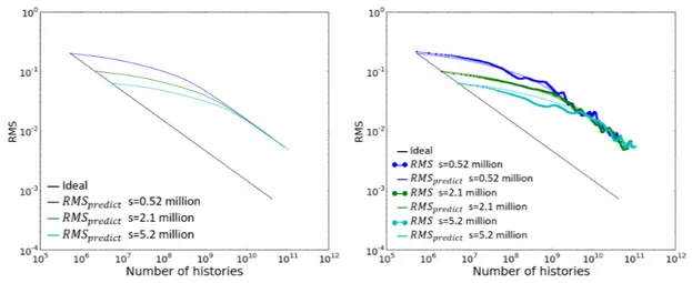
2-5 𝑅𝑀 𝑆 − 𝑁𝑡 curves merge; left: prediction with fitted ACC; right: with

𝑅𝑀 𝑆 data from MC simulation . . . 59

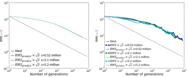
2-6 RMS×√𝑠 − 𝑁 curves overlap; left: prediction with fitted ACC; right: with 𝑅𝑀 𝑆 data from MC simulation . . . 60

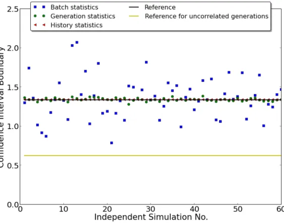
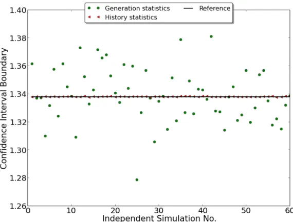
2-7 Comparison of CI evaluated from different methods Batch statistics: Estimate ̂︁𝜎2

𝒳 in 𝑈 𝐵𝐶𝐼 (Eq 2.4.21) with Eq 2.4.22. Generation

statis-tics: Estimate ̂︀𝜎2 _{in 𝐶𝐺𝐶𝐼}

ℎ (Eq 2.4.16) with Eq 2.4.17. History

statis-tics: Estimate ̂︀𝑐2 _{in 𝐶𝐺𝐶𝐼}

𝑁 (Eq 2.4.32) with Eq 2.4.10. . . 70

2-8 Comparison of CI: history and generation statistics . . . 71

(14)

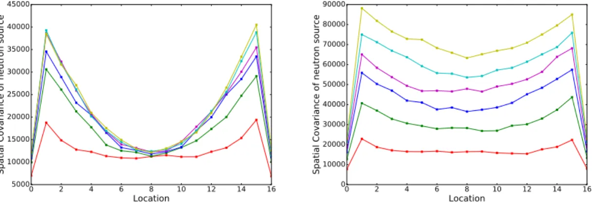
3-1 Variance of tallies as function of location at different generations. . . 80

3-2 Correlation coefficients of tallies as function of location at different generations. . . 81

3-3 Variance of fission source tally of problem TD1 and TD2 . . . 89

3-4 Correlation Prediction from Markov Chain Method and reference of 𝑇 𝐷2 90

3-5 Spatial moments of test problem 𝑇 𝐷1. The solid curves in both figures

correspond to 𝐶𝑖,𝑖(𝑛)−𝜇𝑖(𝑛)𝜇𝑖(𝑛) at generations 𝑛 ∈ {25, 75, 125, 175, 225, 275}

calculated according to Eq 3.3.32 and Eq 3.3.39. . . 102

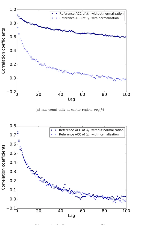
3-6 Correlation coefficients of problem TD1 for tally 𝑍8. The green solid

curve is the predictive model. The green dots are the reference values from independent simulations of problem 𝑇 𝐷1𝑓. The blue crosses are

the corresponding reference correlation coefficients of problem 𝑇 𝐷1𝑛,

where neutron normalization at each generation is enforced. . . 106

3-7 Variances of normalized tally for all regions of problem 𝑇 𝐷1 The solid curves correspond to Var[𝑋𝑖(𝑛)] predicted by Eq 3.3.63 up to order

𝒪 (E𝜖2_{). The dots in Figure 3-7(a) correspond to references calculated}

from simulations without neutron number normalization. The dots in Figure 3-7(b) correspond to references calculated from simulations with neutron number normalization. . . 111

3-8 Correlation coefficients of 𝑋 tallies in problem TD1. The green solid curves correspond to predicted correlation coefficients of 𝜌𝑋,𝐼(𝑘) for

𝐼 = 8 (Figure 3-8(a)) and 𝐼 = 1 (Figure 3-8(b)). The green dots correspond to reference correlation coefficients of 𝑋8 (Figure 3-8(a))

and 𝑋1 from simulations on 𝑇 𝐷1𝑓 (Figure 3-8(b)). The blue crosses

correspond to reference correlation coefficients of 𝑋8 (Figure 3-8(a))

and 𝑋1 from simulations on 𝑇 𝐷1𝑛 (Figure 3-8(b)). . . 114

(15)

3-10 Predicted and Reference 𝐴𝐶𝐶 for the three selected assemblies. The blue diamonds are references calculated from 450 independent simu-lations according to Eq 2.2.41. The black solid curves correspond to the prediction out of the MBP model built from first 8 active gener-ations. The green dashed curves fit the predicted 𝐴𝐶𝐶 to three-term exponential (𝐽 = 3 in Eq 2.3.2). . . 123

3-11 Predicted and Reference variance convergence rate 𝑟(𝑁 )/𝑁 at three selected assemblies. The blue diamonds are references calculated from 450 independent simulations according to Eq 2.2.46. The black solid curves correspond to the prediction out of the quarter-assembly MBP model built from first 8 active generations. The green dashed curves correspond to the calculation from fitting the predicted 𝐴𝐶𝐶 𝜌𝐼(𝑑) up

to 𝑑 = 100 to sum of exponentials.. . . 124

3-12 Predicted and Reference bias of variance at three selected assemblies. The blue diamonds are references calculated from 450 independent simulations according to Eq 2.2.44. The black solid curves correspond to the prediction out of the quarter-assembly MBP model built from first 8 active generations. The green dashed curves correspond to the calculation from fitting the predicted 𝐴𝐶𝐶 𝜌𝐼(𝑑) upto 𝑑 = 100 to sum

of exponentials. . . 125

3-13 Predicted 𝑅𝑀 𝑆 (calculated from variance fully corrected by 𝑟(𝑁 ) and 𝑏(𝑁 )) and Reference 𝑅𝑀 𝑆 at three selected assemblies. The blue diamonds are references calculated from 450 independent simulations according to Eq 2.2.14. The black solid curves correspond to the pre-diction out of MBP model built from first 8 active generations. The green dashed curves correspond to the calculation from fitting the pre-dicted 𝐴𝐶𝐶 𝜌𝐼(𝑑) up to 𝑑 = 100 to sum of exponentials. The green

dots correspond to the 𝑅𝑀 𝑆 prediction if traditional variance estima-tor were used. . . 125

(16)

4-1 Correlation coefficients for central tally region with different sizes in 𝑇 𝐶1 − 1𝐷. The dots correspond to correlation coefficients estimated from independent simulations. The solid line curves correspond to correlation coefficients predicted from the continuous model. . . 145

4-2 Variance convergence rate calculated from underestimation ratio for central tally region with different sizes in 𝑇 𝐶1 − 1𝐷. The dots corre-spond to 𝑟𝐼(𝑛)

𝑛 estimated from independent simulations. The solid line

curves correspond to predictions from the continuous model. . . 147

4-3 Relative square error for central tally region with different sizes in 𝑇 𝐶1 − 1𝐷. The dots correspond to 𝑅𝑆𝐸𝐼 estimated from independent

simulations. The solid line curves correspond to predictions from the continuous model. . . 148

4-4 𝜌𝐼(𝑑) and 𝑟(𝑛)_𝑛 and prediction series truncation. 𝑎 = 20.0𝑐𝑚 is fixed.

The dots correspond to estimation from independent simulations for 𝑇 𝐶1 − 1𝐷. And the solid line curves correspond to prediction with different truncations applied to tally in the central region. . . 150

4-5 Asymptotic variance underestimation ratio for central tally region with different sizes in 𝑇 𝐶1 − 1𝐷. The squares correspond to 𝑟𝐼 estimated

from independent simulations. The dots correspond to predictions from the continuous model with sufficient expansion terms. The diamonds correspond to predictions from the continuous model with the first expansion term. . . 151

4-6 Correlation coefficients for central tally region with different sizes in 𝑇 𝐶1. The dots correspond to correlation coefficients estimated from independent simulations. The solid line curves correspond to correla-tion coefficients predicted from the continuous model. . . 167

4-7 Variance convergence rate calculated from underestimation ratio for central tally region with different sizes in 𝑇 𝐶1. The dots correspond to 𝑟𝐼(𝑛)

𝑛 estimated from independent simulations. The solid line curves

(17)

4-8 Relative square error for central tally region with different sizes in 𝑇 𝐶1. The dots correspond to 𝑅𝑆𝐸𝐼estimated from independent simulations.

The solid line curves correspond to predictions from the continuous model. . . 169

4-9 Asymptotic variance underestimation ratio for central tally region with different sizes in 𝑇 𝐶1. The squares correspond to 𝑟𝐼 estimated from

independent simulations. The dots correspond to predictions from the continuous model with sufficient expansion terms. The diamonds cor-respond to predictions from the continuous model with the first expan-sion term. . . 172

4-10 Correlation coefficients for central tally region with different sizes in 2D BEAVRS. The dots correspond to correlation coefficients estimated from independent simulations. The solid line curves correspond to correlation coefficients predicted from the continuous model. . . 174

4-11 Variance convergence rate for central tally region with different sizes in 2D BEAVRS. The dots correspond to 𝑟𝐼(𝑛)

𝑛 estimated from independent

simulations. The solid line curves correspond to predictions from the continuous model. . . 175

4-12 Asymptotic variance underestimation ratio for central tally region with different sizes in 2D BEAVRS. The squares correspond to 𝑟𝐼 estimated

from independent simulations. The dots correspond to predictions from the continuous model with sufficient expansion terms. . . 176

5-1 Two types of optimization . . . 184

5-2 Source update schemes . . . 187

5-3 Spatial moments on starting delayed scheme, test problem 𝑇 𝐷1 − 𝐷1𝑓 223

5-4 Spatial moments results at active generation 50, 100, 150, 200 and 250, test problem 𝑇 𝐷1 − 𝐷1𝑓 . . . 224

5-5 Correlation coefficients of normalized tallies on test problem 𝑇 𝐷1𝐷1𝑓

(18)

5-6 Variance convergence rate 𝑅(𝑁 )/𝑁 of normalized tallies on test prob-lem 𝑇 𝐷1𝐷1𝑓 and 𝑇 𝐷1𝐷1𝑛 . . . 228

5-7 Var ¯𝑋(𝑁 ) of normalized tallies on test problem 𝑇 𝐷1𝐷1𝑓 and 𝑇 𝐷1𝐷1𝑛 230

5-8 Var ¯𝑋(𝑁 ) of normalized tallies on test problem 𝑇 𝐷1𝑛 and 𝑇 𝐷1𝐷1𝑛 . 231

5-9 Var ¯𝑋(𝑁 ) of normalized tallies on test problem 𝑇 𝐷1 with different delayed neutron schemes. . . 240

5-10 Var ¯𝑋(𝑁 ) of normalized tallies on test problem 𝑇 𝐷1 . . . 241

5-11 Variance and expected Square error (normalized by squared tally ref-erence) of 𝑋 tallies on test problem 𝑇 𝐶1 . . . 242

5-12 bias of ¯𝑋(𝑁 ) of normalized tallies on test problem 𝑇 𝐷1. . . 245

5-13 bias of 𝑋(𝑁 ) of normalized tallies on test problem 𝑇 𝐷1. . . 247

5-14 CDF of neutron age distribution under different delayed neutron schemes249

5-15 bias of normalized tallies and age distribution . . . 252

5-16 𝑅𝑆𝐸𝐼(𝑁 ) vs 𝑁𝑐 with 𝑁0 = 0 . . . 254

5-17 𝑅𝑆𝐸(𝑁 ) vs 𝑁𝑐 with 𝑁0 ∈ {20, 200} and 𝛽 ∈ {0.1, 0.5, 1} in Assembly 2255

5-18 𝑅𝑆𝐸(𝑁 ) vs 𝑁𝑐 with 𝑁0 ∈ {20, 200} and 𝛽 ∈ {0.1, 0.5, 1} in Assembly 3256

5-19 Variance correction under the selected delayed source update scheme. Var[ ¯𝑋(𝑁 )] is plotted as function of active generation number 𝑁 . It can be transformed into function of computation cost as in Figure 5-17 by scaling and shifting the x-axis. . . 259

(19)

List of Tables

2.1 Parameters of demonstration problem . . . 34

2.2 Comparison of Confidence Intervals . . . 65

(20)

(21)

Chapter 1 Introduction

Numerical modeling of neutron physics in nuclear reactors has long played an impor-tant role in the nuclear industry to ensure the safety and reliability of the operating fleet of nuclear reactors and to evaluate the technical capabilities of advanced designs. Monte Carlo methods have long been considered a reference for neutron transport simulations since they make very few approximations in simulating the random walk of neutrons in a system. Monte Carlo simulations permit an accurate representation of the geometry and energy dependence of reaction cross sections and thus provide high-fidelity core spectral calculations.

Previous work has observed correlation effects between neutrons in systems with fission, particularly when performing eigenvalue simulations based on the power iter-ation [3] [22] [17] [42]. In the presence of neutron correlation, Monte Carlo simulation will typically underestimate variance and thus report inaccurate confidence intervals. Correlation will also reduce the tally convergence rate thus requiring many additional generations of neutrons in order to obtain statistically accurate results.

1.1 Background and Literature Review

The general procedure to solve a Monte Carlo eigenvalue problem is described here to introduce the unfamiliar reader to this concept. Individual neutron histories are tracked through an heterogeneous system and information is gathered as they cross

(22)

boundaries and collide with nuclides. At the level of the neutron history, a neu-tron is tracked from birth (source site) to death (absorption or leakage) by sampling path lengths and collision events based on neutron and material properties. In the eigenvalue problem, a number of such neutron histories are grouped into a Fission Source Generation (FSG). In a FSG, when a neutron is terminated by absorption and a fission event is sampled from the cross section data, the fission source site is accumulated into a fission bank for the next FSG. After all neutrons of a generation have been tracked, normalization of the ensuing fission bank is performed to avoid neutron number explosion or extinction. After normalization, a new FSG starts from the normalized fission bank. Once a sufficient number of FSGs (i.e. inactive gener-ations) are performed to achieve a stationary distribution (i.e. distribution follows the fundamental mode), additional FSGs (i.e. active generations) are performed to score tallies of interest. Tallies from all active generations form a sample from which estimate parameters such as 𝑘𝑒𝑓 𝑓, flux, reaction rates and their associated variance can be estimated The procedure is schematically plotted in Fig 1-1.

Figure 1-1: Monte Carlo Eigenvalue Problem Calculation Procedure

If the FGS’s are independent, the variance of the commonly used estimators de-crease inversely proportional to the number of generations (the 1/𝑁 rate). Further if the estimators are unbiased (bias small enough to be neglected when using a large

(23)

gen-eration size [3]), the expected square error decreases with the same 1/𝑁 rate. Previous work has observed correlation effects between neutrons in systems with fission, partic-ularly when performing eigenvalue simulations based on the power iteration [22] [21]. Fig1-2(c)shows the impact of generation-to-generation correlation on the conver-gence rate of a tally on an assembly size mesh for the 2D BEAVRS benchmark [22] [23]. In the presence of correlation, additional generations of neutrons will only slightly im-prove the sample mean and may not be worth the additional effort. In Monte Carlo eigenvalue simulations, quantities of interests are usually estimated as an average over many generations once a stationary fission source is obtained. The sample mean is reported accompanied by an estimate of the variance indicating the level of statistical uncertainty of the simulation and allowing for the definition of confidence intervals. If generation-to-generation correlation is neglected, the variance of the estimator will be evaluated as the variance of the sample of generation tallies divided by 𝑁 , the gen-eration number. This underestimates the variance of the estimator and will report inaccurate confidence intervals.

Neglecting this correlation effect results in an underestimate of uncertainty re-ported by Monte Carlo calculations, the magnitude of which depends on the domi-nance ratio of the problem and the size of the phase space being tallied [46]. The simple approach to avoid underestimation of the variance is to perform multiple in-dependent simulations with different initial random seeds. This will lead to good variance estimates but requires lots of additional work since each independent simu-lation needs an independent fission source and will not improve convergence rates [22]. Another approach is to tally neutrons from batches (one batch contains more than one fission source generations)[13]. This is based on the observation that generation-to-generation correlations decrease as a function of generation lag, which leads to lower correlation between tallies from simulation batches than those from genera-tions. The many-generations-in-one-batch method provides a better estimate of the variance with a single simulation at the cost of many more generations. The super-history method [3] tracks each neutron through more than one generations (instead of just one) before any fissions are banked for the next batch. This is similar to the

(24)

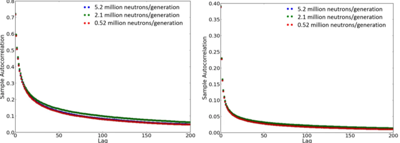
(a) Autocorrelation coefficients assembly-size tally

(b) Autocorrelation coefficients pin-size tally

(c) RMS Convergence assembly-size tally

Figure 1-2: Plots of autocorrelation coefficients and convergence rate of assembly-size tally on 2D BEAVRS. Generation-to-generation correlation makes statistical error deviate from ideal convergence rate. (From "Monte Carlo and Thermal Hydraulic Coupling using Low-Order Nonlinear Diffusion Acceleration" by B. Herman, 2014 [22] )

many-generation-in-one-batch method except that tallies are only performed on the last generation in each batch. Wielandt’s method, originally developed for deter-ministic nuclear reactor calculations [7] [37] was applied to Monte Carlo eigenvalue calculation [6] by tacking some neutron for more than one generations in one batch. Wielandt shift method reduces correlation by effectively solving a different problem with lower eigenvalues. This method requires an estimate of the upper bound of the eigenvalue. Significant reduction requires a compact estimate of the upper bound.

The generation-to-generation correlation of tally 𝑋 between generation 𝑛 and 𝑛 + 𝑘 can be directly characterized by the covariance matrix of a tally from different

(25)

generations.

𝜌(𝑛, 𝑛 + 𝑘) = Cov[𝑋(𝑛), 𝑋(𝑛 + 𝑘)]

√︀Var[𝑋(𝑛)] Var[𝑋(𝑛 + 𝑘)] (1.1.1)

When the generation tally values can be viewed as stationary time series, the covari-ance between generations only depends on generation distcovari-ance or lag [47] [22].

𝜌(𝑛, 𝑛 + 𝑘) = 𝜌(𝑛; 𝑘) = 𝜌(𝑘) (1.1.2)

In recent years, more effort has been dedicated at evaluating the auto-correlation coefficients (ACC) observed in the Monte Carlo eigenvalue simulations. Recent work by Herman [21] [22] extensively demonstrated the impact of generation-to-generation correlations on a realistic 2D full core PWR benchmark. This work also numerically showed the dependency on the mesh size as well as the insensitivity to the number of neutrons per generation (Figure 1-2(a) and Figure1-2(b)).

Previous work has also proposed methods to predict the underestimation ratio between the correlated and uncorrelated estimates. The investigated methods can be classified into two categories. The first performs data fitting on simulation outputs to capture the correlation. The second directly computes covariance between the Monte Carlo generations based on corresponding approximations of the Monte Carlo simulation [44]. Demaret et al [14] fitted AR (auto-regressive) and MA (Moving Average) models to the results of Monte Carlo eigenvalue calculations and used the AR and MA models to give variance estimator of 𝑘𝑒𝑓 𝑓. Yamamoto et al [49] [50] expanded the fission source distribution with diffusion equation modes, performed numerical simulation of the AR process of the expansion coefficients and used the correlation of the AR process to predict the Monte Carlo eigenvalue simulation. Approximating the original neutron transport problem with a diffusion problem lead to a non-negligible lost in accuracy. Inspired by Brissenden and Garlick’s work [3], Sutton [42] applied the discretized phase space (DPS) approach to predict the underestimation ratio but the method cannot predict the ratio when one neutron generates offspring in different

(26)

phase space regions or generates a random number of offspring. Ueki [45] developed variance estimator with orthonormally weighted standardized time series (OWSTS). The estimator is based on the convergence of step-wise interpolation of standardized tallies (SIST) to a Brownian bridge. SIST weighted by a trigonometric family of weighting functions gives a new statistical estimator for the variance. Asymptotic behavior of the expectation of the new estimator leads to a variance estimator that is not affected by the correlation effect thus converging at a 1/N rate. Numerical results showed that the variance can be accurately estimated after approximately 5000 ∼ 10000 active generations for problems with non-negligible auto-correlation up to 100 generation lags (as observed in a typical LWR). A convergence diagnosis is also necessary to determine when the asymptotic behavior is reached. However, the convergence diagnosis cannot be implemented on-the-fly.

In summary, among the current methods to reduce the impact of correlations, the methods that decorrelate batches become very costly due to an increase in the number of generations. The methods that correct the variance underestimation using post-processing techniques are very memory intensive since tallies of all active generations need to be stored. Finally, the methods that predict the correlation coefficients and thus correct the variance with approximate models do not capture a sufficient level of accuracy.

Previous work also proposes quantitative explanations of the generation-to-generation of tallies. Dumonteil et al [18] attributed the generation-to-generation correlation to spatial correlation of the fission process and ensuing asymmetry between neutron cre-ation and annihilcre-ation in a stochastic branching process. Houchmandzadeh [24] and Zoia [51] investigated the issue of neutral particle clustering, the phenomenon where particles without interaction can concentrate locally. In simple homogeneous prob-lems, spatial covariance between particle number density at different positions proves existence of clustering theoretically and thus explains the existence of generation-to-generation correlation of tallies contributed by these clustered particles.

(27)

1.2 Thesis Objectives

The subject matter of this thesis is organized along three main themes:

∙ Correlation Analysis – Quantify correlation coefficients in different problems, analyze the effect of correlations on variance estimation, analyze the dependency of correlation on problems and simulation parameters. The goal is to understand the nature of the correlations and determine appropriate variance estimators if the correlations are known.

∙ Correlation prediction – Develop models to predict correlation coefficients as a function of tally position, region and simulation parameters accurately without storing all tallies. The goal is to develop a simple deterministic model that can predict correlations prior to performing the bulk of the simulation thus providing an accurate estimate of the variance correction needed and an estimate as to when the desired level of accuracy will be reached.

∙ Run Strategy in the presence of correlations – Allocate computation resources in optimal ways to reach better results given cost requirement. The goal is to develop a simple diagnosis indicating the need for corrective action, and once identified, provide an optimal run strategy to achieve the target accuracy faster.

1.3 Thesis Outline

Chapter 2 discusses the correlation coefficients of tallies in Monte Carlo simulations and their impact on the underestimation of variances. Behavior of correlation coef-ficients and variance underestimation ratios are analyzed in different situations. A post-processing method is proposed by assuming the correlation coefficients 𝜌(𝑛; 𝑘) do not depend on generation 𝑛 and decrease exponentially as a function of the gener-ation lag 𝑘. This method estimates correlgener-ation coefficients from all tallies and fits the estimated correlation coefficients to exponentials. The fitted correlation coefficients can accurately predict variance of accumulated tallies at any generation 𝑛. The fitted

(28)

correlation coefficients also explain the particular features of the variance convergence rates observed numerically.

Chapter 3 focuses on predicting correlation coefficients before starting the active generations of the simulation. This provides not only correction to the underestimated variance but also provides an estimate on when a target accuracy will be reached. A Markov Chain Monte Carlo model is developed to show that the dependence of neutron source bank between consecutive generations contributes a significant fraction of the correlation of tallies between generations but also misses an important part caused by the multiplying effect of fission. The method of multitype branching process (MBP) is developed to capture both the source bank dependence and the correlation due to multiplication. The MBP model is exact in predicting correlations for neutrons transported in a discrete phase space and provides acceptable accuracy in continuous problems by constructing an approximate discrete problem from tallies. Since the MBP model is a discrete approximation, it can predict correlations and variances on tally meshes coarser than the discretized model mesh accurately.

Chapter 4 provides a prediction model of the correlation level at any mesh size without the requirement of high accuracy discrete tallies in order to quickly determine if variance correction is needed. This chapter generalizes the MBP model to a contin-uous space and solves correlation coefficients (and thus variance correction factors) exactly in a homogeneous problems. The real heterogeneous problem can then be homogenized while imposing preservation of the neutron migration area. The corre-lation coefficients and asymptotic variance underestimation ratio of the homogenized problem can give a rough estimate of those in the real problem.

Chapter 5 investigates how to modify the current Monte Carlo eigenvalue sim-ulations to reduce the impact of correlations and improve the variance convergence rate in the active generations. For a given active generation size, more neutrons are simulated in the inactive generations to enable a split of the source bank into two parts, neutrons in one part are transported in every active generation (i.e. prompt bank) and contribute to tallies, neutrons in the other bank (i.e. delayed bank) are car-ried forward until included in the prompt at later generations. The delayed neutron

(29)

method provides better variance behavior at the cost of more work in the inactive generations. A predictive model for the delayed scheme is also developed to help identify an optimal run strategy and provide an estimate of the variance correction.

(30)

(31)

Chapter 2 Estimating Correlation and

Correcting Variance

2.1 Problems for Illustration

Since performing meaningful analysis on a large problem is inherently difficult, this section defines two simple problems to illustrate the impact of correlations and provide references for the predictive methods developed in this work.

The first problem tracks neutrons in discrete phase space regions and has an analytic solution that can easily be used to evaluate spatial and temporal moments, and correlation coefficients of tallies.

The problem is also characterized by simple parameters which facilitates the in-terpretation of the observed correlation induced behavior. This test problem will be referred to as 𝑇 𝐷1(discrete test problem) in the following chapters.

The second problem tracks neutrons in a simple homogeneous reflective cube with constant (one group) cross section. This problem has an exact solution for flux and reaction rates. The geometry and material properties of the cube are selected to be representative of and exhibit similar behavior to the full core PWR by matching the migration area of neutrons of a typical LWR.

This test problem will be referred to as 𝑇 𝐶1(continuous test problem) in the following chapters.

(32)

2.1.1 Neutrons in Discrete Phase Space

In the first problem, neutrons are being transferred among 𝑀 phase space regions. The process is specified by a Markov Chain transfer matrix 𝑃 , with 𝑃𝑖,𝑗 being the probability that a neutron at region 𝑖 will be in region 𝑗 in the next generation and a random variable 𝜉𝑖 representing new neutrons per fission at region 𝑖 with 𝑝𝑖,𝑎 being the probability that a fission at region 𝑖 produces 𝑎 new neutrons.

In OpenMC [39], like in many other Monte Carlo codes, the fission process is simulated by first evaluating the expected number of neutrons per fission

𝜈 ≡ E[𝜉 |𝜉 ̸= 0] (2.1.1)

where 𝜉 denotes the random variable of new neutrons per absorption and adding the condition 𝜉 ̸= 0 makes the conditional expectation equal to the expected number of new neutrons per fission.

Then sample ⌈𝜈⌉ (the closest integer that is larger than or equal to 𝜈) and ⌊𝜈⌋ (the closest integer that is smaller than or equal to 𝜈) with appropriate probability to satisfy the constraint on expectation of 𝜉 (Eq 2.1.1).

That is, after a neutron is determined to induce a fission event and the expected number of new neutrons per fission is determined to be 𝜈, the number of new neutrons is sampled to be ⌈𝜈⌉ with probability 𝑝′_⌈𝜈⌉ and ⌊𝜈⌋ with probability 𝑝′_⌊𝜈⌋ such that

⌊𝜈⌋𝑝′_⌊𝜈⌋+ ⌈𝜈⌉𝑝′_⌈𝜈⌉ = 𝜈 (2.1.2)

In the simple test problem, it is not necessary to simulate the neutrons as above by first determining whether the neutron induces a capture or fission event then determining the number of new neutrons per fission. The test problem specifies the probability of number of new neutrons per absorption directly. Then the distribution

(33)

of 𝜉𝑖 can be solved from the below equations ∑︁ 𝑎 𝑝𝑖,𝑎= 1 ∑︁ 𝑎 𝑎 𝑝𝑖,𝑎= E𝜉 ∑︁ 𝑎 𝑎 𝑝𝑖,𝑎 1 − 𝑝𝑖,0 = 𝜈𝑖 (2.1.3)

If a further assumption is made to make the system critical, that is E𝜉 = 1. The probabilities are determined as

𝑝𝑖,0 = 1 − 1 𝜈𝑖 𝑝𝑖,⌊𝜈⌋ = ⌈𝜈⌉ − 𝜈 𝜈 𝑝𝑖,⌈𝜈⌉ = 𝜈 − ⌊𝜈⌋ 𝜈 𝑝𝑖,𝑎 = 0 (𝑜𝑡ℎ𝑒𝑟𝑤𝑖𝑠𝑒) (2.1.4)

where the material is assumed to be fissile and the equations above will only be applied to test problems with fissile material.

The numerical values of the matrix 𝑃 are selected such that 𝑃𝑖,𝑖 = 0.5

𝑃𝑖,𝑖−1 = 𝑃𝑖,𝑖+1 = 0.25 (𝑖 > 1, 𝑖 < 𝑀 )

𝑃1,2 = 𝑃𝑀,𝑀 −1= 0.5

𝑃𝑖,𝑗 = 0 (𝑜𝑡ℎ𝑒𝑟𝑤𝑖𝑠𝑒)

(2.1.5)

where the 𝑀 phase space regions are indexed from 1 to 𝑀 .

It can be shown that the Markov matrix specified according to Eq 2.1.5 has the normalized equilibrium distribution 𝜋 with

(34)

Table 2.1: Parameters of demonstration problem

Geometry 𝜈 Macro Cross-Section 𝑘𝑒𝑓 𝑓

Boundary Width(cm) Σ𝑠(𝑐𝑚−1) Σ𝑐(𝑐𝑚−1) Σ𝑓(𝑐𝑚−1) Σ𝑡(𝑐𝑚−1) Reflective 400 2.45 0.270 0.018 0.012 0.300 1 𝜋𝑖 = 1 𝑀 − 1 (𝑖 = 2, · · · , 𝑀 − 1) 𝜋𝑖 = 1 2(𝑀 − 1) (𝑖 = 1, 𝑀 ) (2.1.6)

For any given neutron at region 𝑖, the destination region 𝑗 is sampled according to 𝑃𝑖,𝑗. Then for the neutron absorbed at region 𝑗, the number of new neutrons 𝑎 is sampled according to 𝑝𝑗,𝑎. The 𝑎 neutrons in region 𝑗 will then be transferred to new locations as described above.

2.1.2 Neutrons in a Homogeneous Cube

This problem is designed to mimic the correlation behavior of real PWR neutron eigenvalue simulation. Analyzing correlation coefficients on a full core realistic prob-lem is a very costly endeavor. Herman et al [22] were able to compute such coefficients on the 2D BEAVRS benchmark using extensive computational time making any sub-stantive analysis impractical. In order to accelerate the process, a simple benchmark was developed that preserves the correlation effects, reduces run time and has a simple analytical reference solution of neutron distribution. Parameters of the homogenized cubic reactor are given in Table 2.1. The simple benchmark was chosen as a 400𝑐𝑚 reflective cube since it has dimensionality similar to that of a full core PWR. Addi-tionally, the one group cross sections were selected such that the system is critical and preserves the migration length of neutrons.

In this problem, neutrons are not transferred among discrete states but instead within a continuous phase space in a realistic way. The transfer probability density

(35)

for a collision from position 𝑥 to 𝑥′ is defined as

𝑃 (𝑥, 𝑥′) = Σ𝑡𝑒−Σ𝑡|𝑥−𝑥

′_|

(2.1.7)

The probability mass function of new neutrons after an absorption event at any position is 𝑝0 = Σ𝑐 Σ𝑎 𝑝1 = 0 𝑝2 = Σ𝑓 Σ𝑎 0.55 𝑝3 = Σ𝑓 Σ𝑎 0.45 𝜈 = 0.55 × 2 + 0.45 × 3 (2.1.8)

where 𝑝0 is the probability of neutron capture, 𝑝2 and 𝑝3 represent a probability for producing a discrete number of neutrons from fission.

The stochastic behavior of fission events in the simple benchmark can be evaluated analytically. For a tally region 𝑚 occupying 𝜂𝑚fraction of volume of the whole system, the expected number of fission events 𝑍𝑚 induced by 𝑠 independent neutrons is

⟨𝑍𝑚⟩ = 𝑠 Σ𝑓 Σ𝑡− Σ𝑠

𝜂𝑚 (2.1.9)

where Σ𝑡, Σ𝑓, Σ𝑠 are the total cross section, fission cross section, scattering cross section of the cube respectively. And the variance of 𝑍𝑚 is

Var[𝑍𝑚] = 𝑠 Σ𝑓𝜂𝑚 Σ𝑎 (︂ 1 − Σ𝑓𝜂𝑚 Σ𝑎 )︂ (2.1.10)

Derivation of the expectation and variance of 𝑍𝑚 is shown in AppendixA1.1.

To analyze this benchmark a simple Monte Carlo code was developed on a GPU to accelerate the analysis. The number of neutrons at each generation is equal to the

(36)

number of threads (number of blocks times number of threads per block) launched. Each thread has a local collision tally in each spatial bin and a reduction algorithm is performed after each generation to obtain the global tally. When the generation size (number of neutrons per generation) exceeds the number of threads on the GPU, kernels are launched sequentially. Generation sizes are selected to the power of 2 for more efficient use of the GPU hardware. The fission source distribution is then obtained by multiplying the collision source distribution by the constant factor Σ𝑓

Σ𝑡.

2.2 Background

2.2.1 Variance of correlated sample average

In Monte Carlo eigenvalue simulations, quantities of interests are usually estimated as an average over many generations once a stationary fission source is obtained. The sample mean is reported accompanied by an estimate of the variance indicating the level of statistical uncertainty of the simulation and allowing for the definition of confidence intervals.

2.2.1.1 Correlation coefficients in variance underestimation For tally 𝑋, by definition, the variance of the sample mean is given by

Var[︀𝑋(𝑁 )]︀ = Var¯ ⎡ ⎢ ⎢ ⎣ 𝑁 ∑︀ 𝑛=1 𝑋(𝑛) 𝑁 ⎤ ⎥ ⎥ ⎦ = 1 𝑁2 Var [︃ _𝑁 ∑︁ 𝑛=1 𝑋(𝑛) ]︃ = 1 𝑁2E ⎡ ⎣ (︃ _𝑁 ∑︁ 𝑛=1 𝑋(𝑛) − E [︃ _𝑁 ∑︁ 𝑛=1 𝑋(𝑛) ]︃)︃2⎤ ⎦ (2.2.1)

where 𝑋(𝑛) is the result obtained from generation 𝑛 and 𝑁 is the total number of active generations.

(37)

groups of terms Var[︀𝑋(𝑁 )]︀ =¯ 1 𝑁2 (︃ ∑︁ 𝑛 E[︀(𝑋(𝑛) − E[𝑋(𝑛)])2]︀ + ∑︁ 𝑛̸=𝑗 E [(𝑋(𝑛) − E[𝑋(𝑛)])(𝑋(𝑗) − E[𝑋(𝑗)])] )︃ = 1 𝑁2 (︃ 𝑁 𝜎2+ 2∑︁ 𝑛<𝑗 Cov [𝑋(𝑛), 𝑋(𝑗)] )︃ (2.2.2) where {𝑋(𝑛)}𝑁

𝑛=1 is assumed to have identical distribution and 𝜎2 is the variance of 𝑋(𝑛) for any 𝑛.

𝜎2 = Var[𝑋(𝑛)] ∀𝑛 (2.2.3)

If further assumptions are made that the generations are uncorrelated, as often assumed in Monte Carlo simulations, the covariance terms would vanish and the variance of the sample mean would be

Var[ ¯𝑋(𝑁 )] = 𝜎 2

𝑁 (2.2.4)

In the presence of correlation, since the generation tally values can be modeled as stationary time series, the covariance between two batches only depends on batch distance or lag, 𝑘, [22] [47] Var[︀𝑋(𝑁 )]︀ =¯ 1 𝑁2 (︃ 𝑁 𝜎2+ 2 𝑁 −1 ∑︁ 𝑘=1 𝑁 −𝑘 ∑︁ 𝑖=1 Cov[𝑋(𝑖), 𝑋(𝑖 + 𝑘)] )︃ = 1 𝑁2 (︃ 𝑁 𝜎2+ 2 𝑁 −1 ∑︁ 𝑘=1 (𝑁 − 𝑘) Cov[𝑋(𝑖), 𝑋(𝑖 + 𝑘)] )︃ (2.2.5)

where the first equality restructures the summation over indices 𝑖, 𝑗 into 𝑖, 𝑗 = 𝑖 + 𝑘 with 𝑘 being the generation lag, the second equality recognizes the 𝑁 − 𝑘 identical covariance terms Cov[𝑋(𝑖), 𝑋(𝑖 + 𝑘)] based on the stationarity assumption.

Taking into account the covariance between generations, the variance of the sample mean of observable 𝑋 can be evaluated with Eq 2.2.6, where 𝜎2 is the variance of

(38)

𝑋, 𝑁 is the number of active generations, and 𝜌(𝑘) is the autocorrelation coefficient between 𝑋’s with generation lag 𝑘.

Var[ ¯𝑋] = 𝜎 2 𝑁 (︃ 1 + 2 𝑁 −1 ∑︁ 𝑘=1 (︂ 1 − 𝑘 𝑁 )︂ 𝜌(𝑘) )︃ (2.2.6) 𝜌(𝑘) = 𝜌(𝑛; 𝑘) = 𝜌(𝑛, 𝑛 + 𝑘) = Cov[𝑋(𝑛), 𝑋(𝑛 + 𝑘)] √︀Var[𝑋(𝑛)] Var[𝑋(𝑛 + 𝑘)] (2.2.7)

It is worthwhile to note that 𝜌(𝑘) should have been more naturally written as Cov[𝑋(𝑖), 𝑋(𝑖+ 𝑘)]/𝜎2_{following the derivation above. 𝜎}2_{is expanded back into}_{√︀Var[𝑋(𝑖)] Var[𝑋(𝑖 + 𝑘)]} with the stationarity assumption in order to make 𝜌(𝑘) match the definition of the Pearson correlation coefficient [9].

As can be seen from Eq 2.2.6, if the variance of the sample formed by the gener-ation results {𝑋(1), · · · , 𝑋(𝑁 )} is divided by the total number of active genergener-ations 𝑁 to estimate the variance of their average, the variance of the estimator is underes-timated by a factor 𝑟(𝑁 ) defined as

𝑟(𝑁 ) ≡ Var[ ¯𝑋(𝑁 )] Var[𝑋] = 1 + 2 𝑁 −1 ∑︁ 𝑘=1 (︂ 1 − 𝑘 𝑁 )︂ 𝜌(𝑘) (2.2.8)

where 𝑟(𝑁 ) < 𝑁 unless 𝜌(𝑘) = 1 for all k.

2.2.1.2 Correlation coefficients in predicting 𝑅𝑀 𝑆

When estimating observable 𝑋 (with expectation ⟨𝑋⟩) by estimator ˆ𝑋, it can be shown that the expected square error (ESE) equals the variance of the variable plus the bias of the estimator.

𝐸𝑆𝐸 = E[( ˆ𝑋 − ⟨𝑋⟩)2] = Var[ ˆ_{𝑋] + (E[ ˆ}𝑋] − ⟨𝑋⟩)2 (2.2.9)

If the estimator is unbiased, the expected square error becomes

(39)

Eq 2.2.10 shows the equivalence between square error and variance of estimator. Therefore, the error and convergence rate of the estimator (the sample mean) can be predicted by its 𝐸𝑆𝐸 or variance. The 𝐸𝑆𝐸 can be used as a predictor for the 𝑅𝑀 𝑆 as follows.

First, from the above unbiasedness assumption, for any tally in region 𝑚, the expectation of square error is equal to the variance

𝐸𝑆𝐸𝑚 = Var[ ˆ𝑋𝑚] (2.2.11)

One common metric of interest is the relative square error (RSE),

𝑅𝑆𝐸𝑚 =

( ˆ𝑋𝑚− ⟨𝑋𝑚⟩)2 ⟨𝑋𝑚⟩2

(2.2.12)

whose expectation is related to the variance as before

𝐸[𝑅𝑆𝐸𝑚] = 𝐸𝑆𝐸𝑚 ⟨𝑋𝑚⟩2 = Var[ ˆ𝑋𝑚] ⟨𝑋𝑚⟩2 (2.2.13)

This work focuses on predicting variance, and the predicted variance is used as an approximation of 𝑅𝑆𝐸.

𝑅𝑆𝐸𝑚,𝑝𝑟𝑒𝑑𝑖𝑐𝑡 =

Var[ ˆ𝑋𝑚] ⟨𝑋𝑚⟩2

(2.2.14)

Finally, a global metric of error is constructed as spatially averaging the 𝑅𝑆𝐸𝑚 for each region.

𝑅𝑀 𝑆 = ⎯ ⎸ ⎸ ⎸ ⎷ 𝑀 ∑︀ 𝑚=1 𝑅𝑆𝐸𝑚 𝑀 (2.2.15)

where the subscript 𝑚 denotes index of a tally region, 𝑀 is the total number of tally regions; 𝑅𝑀 𝑆 stands for Root Mean Square error, since it is the square root of average of the relative square error over all tally regions. 𝑅𝑀 𝑆 synthesizes the relative square error of all tally regions into a one number metric.

(40)

prediction 𝑅𝑀 𝑆𝑝𝑟𝑒𝑑𝑖𝑐𝑡 = ⎯ ⎸ ⎸ ⎸ ⎷ 𝑀 ∑︀ 𝑚=1 𝑅𝑆𝐸𝑚,𝑝𝑟𝑒𝑑𝑖𝑐𝑡 𝑀 = √︀ E[𝑅𝑀 𝑆2] (2.2.16)

If the generation average ¯𝑋𝑚(𝑁 ) is selected to be the estimator ˆ𝑋𝑚 = ¯𝑋𝑚(𝑁 ), the variance of the estimator can be expanded using the definition in Eq2.2.6. Thus, the predicted 𝑅𝑀 𝑆 can be written as:

𝑅𝑀 𝑆𝑝𝑟𝑒𝑑𝑖𝑐𝑡 = ⎯ ⎸ ⎸ ⎷ 1 𝑀 𝑀 ∑︁ 𝑚=1 Var[ ¯𝑋𝑚(𝑁 )] ⟨𝑋𝑚⟩2 = ⎯ ⎸ ⎸ ⎷ 1 𝑀 𝑁 𝑀 ∑︁ 𝑚=1 𝜎2 𝑚 ⟨𝑋𝑚⟩2 (︃ 1 + 2 𝑁 −1 ∑︁ 𝑘=1 (︂ 1 − 𝑘 𝑁 )︂ 𝜌𝑚(𝑘) )︃ (2.2.17)

Switching the order of summation over tally regions and summation over active generations, Eq2.2.17can be expressed in a neat way hiding tally region dependence, which eases later analysis. By defining an average variance for all tally regions as

¯ 𝜎2 ₌ 1 𝑀 𝑀 ∑︁ 𝑚=1 𝜎2 𝑚 ⟨𝑋𝑚⟩2 (2.2.18)

and an average variance-weighted ACC,

¯ 𝜌(𝑘) = 𝑀 ∑︀ 𝑚=1 𝜎2 𝑚 ⟨𝑋𝑚⟩2𝜌𝑚(𝑘) 𝑀 ∑︀ 𝑚=1 𝜎2 𝑚 ⟨𝑋𝑚⟩2 (2.2.19)

the predicted 𝑅𝑀 𝑆𝑝𝑟𝑒𝑑𝑖𝑐𝑡 can be cast in the same form as Eq 2.2.6

𝑅𝑀 𝑆𝑝𝑟𝑒𝑑𝑖𝑐𝑡 = ⎯ ⎸ ⎸ ⎷ ¯ 𝜎2 𝑁 (︃ 1 + 2 𝑁 −1 ∑︁ 𝑘=1 (1 − 𝑘 𝑁) ¯𝜌(𝑘) )︃ (2.2.20)

(41)

pre-dicting the convergence rate of the tallies as a function of the number of generations, 𝑁 , and the number of neutrons per generation, via the ¯𝜎2 _term.

2.2.2 Bias of Sample Variance Estimated from Generation

Tal-lies

Eq 2.2.20shows that the variance, ¯𝜎2_{, divided by the sample size, 𝑁 , underestimates} the variance of the mean. On the other hand, if the variance is unknown, it must be estimated from samples that are correlated. This section provides the correction to the variance estimator needed to take into account sample correlation.

For a sample of observables of random variable 𝑋, {𝑋(1), · · · , 𝑋(𝑁 )}, sample variance ̂︀𝑠2 _{is a common estimate of variance of 𝑋 [}₃₄_].

̂︀ 𝑠2_{(𝑁 ) =} 1 𝑁 𝑁 ∑︁ 𝑛=1 (𝑋(𝑛) − ¯𝑋(𝑁 ))2 = 𝑁 ∑︀ 𝑛=1 𝑋(𝑛)2 𝑁 − ⎛ ⎜ ⎜ ⎝ 𝑁 ∑︀ 𝑛=1 𝑋(𝑛) 𝑁 ⎞ ⎟ ⎟ ⎠ 2 = 1 𝑁 𝑁 ∑︁ 𝑛=1 𝑋(𝑛)2− 1 𝑁2 𝑁 ∑︁ 𝑛,𝑛′₌₁ 𝑋(𝑛)𝑋(𝑛′) = 1 𝑁 𝑁 ∑︁ 𝑛=1 𝑋(𝑛)2− 1 𝑁2 (︃ _𝑁 ∑︁ 𝑛=1 𝑋(𝑛)2+∑︁ 𝑛̸=𝑛′ 𝑋(𝑛)𝑋(𝑛′) )︃ (2.2.21)

The derivation below finds the expectation of the sample variance under different assumptions and adjusts it to be an unbiased estimator.

Expectation of ̂︀𝑠2 _{in Eq} _2.2.21 _{can be first expanded to}

E ̂︀𝑠2(𝑁 ) = 1 𝑁 𝑁 ∑︁ 𝑛=1 E[︀𝑋(𝑛)2]︀ − 1 𝑁2 (︃ _𝑁 ∑︁ 𝑛=1 E[︀𝑋(𝑛)2]︀ + ∑︁ 𝑛̸=𝑛′ E [𝑋(𝑛)𝑋(𝑛′)] )︃ (2.2.22)

The factor after _𝑁1 in Eq 2.2.22 contains 𝑁 terms. The factor after _𝑁12 in Eq 2.2.22

(42)

summation contains 𝑁 (𝑁 − 1) pairs.

Assume E[𝑋(𝑛)] does not change over generation 𝑛 and denote it with E[𝑋]. Subtracting E[𝑋]2 from both terms on RHS of Eq 2.2.22 leads to Eq2.2.23.

E ̂︀𝑠2(𝑁 ) = 1 𝑁 {︃ _𝑁 ∑︁ 𝑛=1 E[︀𝑋(𝑛)2]︀ − 𝑁 E[𝑋]2 }︃ − 1 𝑁2 (︃ _𝑁 ∑︁ 𝑛=1 E[︀𝑋(𝑛)2]︀ + ∑︁ 𝑛̸=𝑛′ E [𝑋(𝑛)𝑋(𝑛′)] − 𝑁2E[𝑋]2 )︃ (2.2.23)

Then merge the 𝑁 number of E[𝑋]2terms back to the summation indexed from 𝑛 = 1 to 𝑁 . Among the 𝑁2 _{number of E[𝑋]}2 _{terms, merge 𝑁 of them are to the summation} indexed by 𝑛, merge the remaining 𝑁 (𝑁 − 1) to the summation indexed by 𝑛, 𝑛′. Expectation of ̂︀𝑠2_{(𝑁 ) is now written as}

E ̂︀𝑠2(𝑁 ) = 1 𝑁 𝑁 ∑︁ 𝑛=1 {︀ E[︀𝑋(𝑛)2]︀ − E[𝑋]2}︀ − 1 𝑁2 {︃ _𝑁 ∑︁ 𝑛=1 (︀ E[︀𝑋(𝑛)2]︀ − E[𝑋]2)︀ + ∑︁ 𝑛̸=𝑛′ (︀ E [𝑋(𝑛)𝑋(𝑛′)] − E[𝑋]2)︀ }︃ (2.2.24)

Since E𝑋 = E𝑋(𝑛) for any 𝑛, recover E𝑋 as E𝑋(𝑛) or E𝑋(𝑛′) in Eq2.2.24whenever needed to match the summation index. The expectations with matched generation indices 𝑛 and 𝑛′ in Eq2.2.25 are simplified to covariances.

E ̂︀𝑠2(𝑁 ) = 1 𝑁 𝑁 ∑︁ 𝑛=1 {︀ E[︀𝑋(𝑛)2]︀ − E[𝑋(𝑛)]2}︀ − 1 𝑁2 {︃ _𝑁 ∑︁ 𝑛=1 (︀ E[︀𝑋(𝑛)2]︀ − E[𝑋(𝑛)]2)︀ + ∑︁ 𝑛̸=𝑛′ (E [𝑋(𝑛)𝑋(𝑛′)] − E[𝑋(𝑛)]E[𝑋(𝑛′)]) }︃ (2.2.25) = 1 𝑁 𝑁 ∑︁ 𝑛=1 Var[𝑋(𝑛)] − 1 𝑁2 (︃ _𝑁 ∑︁ 𝑛=1 Var[𝑋(𝑛)] +∑︁ 𝑛̸=𝑛′ Cov[𝑋(𝑛), 𝑋(𝑛′)] )︃ (2.2.26)

(43)

When simplifying Eq 2.2.25 to Eq2.2.26, the following equations are used.

Var[𝑋] = E[𝑋2] − E[𝑋]2 Cov[𝑋, 𝑋′_{] = E[𝑋𝑋}′_{] − E𝑋E𝑋}′

(2.2.27)

The above derivation holds for any processes {𝑋(𝑛)}𝑁

𝑛=1 with constant E𝑋(𝑛). In the three sections below, Eq 2.2.22 is applied to relate the ̂︀𝑠2 _{to useful variance} estimators under different assumptions: independent identical 𝑋(𝑛), correlated but identical 𝑋(𝑛) and correlated 𝑋(𝑛) with only identical E𝑋(𝑛).

2.2.2.1 Independent and identical observables

If we assume that {𝑋(𝑛)}𝑁_𝑛=1 belong to an identical distribution and are uncorrelated, all the Var[𝑋(𝑛)] terms are identical and equal to Var[𝑋]. This leads to the covariance term vanishing which simplifies Eq 2.2.26 to

E ̂︀𝑠2(𝑁 ) = 𝑁 − 1

𝑁 Var[𝑋] (2.2.28)

This reveals the classic unbiased variance estimator for uncorrelated samples [9]:

̂︀ 𝜎2

0(𝑁 ) = ̂︀𝑠2(𝑁 ) 𝑁

𝑁 − 1 (2.2.29)

2.2.2.2 Correlated but identical observables

If the observables are correlated but still with identical Var[𝑋(𝑛)] terms, Eq2.2.26is simplified to E ̂︀𝑠2(𝑁 ) = Var[𝑋] (︃ 1 𝑁𝑁 − 1 𝑁2 (︃ 𝑁 +∑︁ 𝑛̸=𝑛′ Cov[𝑋(𝑛), 𝑋(𝑛′)] Var[𝑋] )︃)︃ = Var[𝑋] 𝑁 (︃ 𝑁 − (︃ 1 + 1 𝑁 ∑︁ 𝑛̸=𝑛′ Cov[𝑋(𝑛), 𝑋(𝑛′)] √︀Var[𝑋(𝑛)] Var[𝑋(𝑛′_)] )︃)︃ = Var[𝑋] 𝑁 (︃ 𝑁 − (︃ 1 + 𝑁 −1 ∑︁ 𝑘=1 (︂ 1 − 𝑘 𝑁 )︂ 𝜌(𝑘) )︃)︃ (2.2.30)

(44)

where the last equality follows the same assumption that generation-to-generation correlation coefficient depends only on generation lag as in Eq 2.2.5. The definition of variance underestimation ratio 𝑟(𝑁 ) (Eq 2.2.8) is recognized in Eq 2.2.30. After re-organization, this leads to the unbiased variance estimator for correlated sample with identical distribution

𝜎₁2(𝑁 ) = ̂︀𝑠2_{(𝑁 )} 𝑁

𝑁 − 𝑟(𝑁 ) (2.2.31)

where 𝜌(𝑘) (and therefore 𝑟(𝑁 )) are assumed to be known parameters rather a statis-tic calculated from the sample {𝑋(𝑛)}𝑁

𝑛=1.

Comparing ̂︀𝜎2

1 (Eq2.2.31) and ̂︀𝜎02(Eq 2.2.29) shows that the bias of the estimator ̂︀

𝜎2

0 is related with the variance underestimation ratio 𝑟 through

𝑏(𝑁 ) ≡ 𝜎̂︀ 2 0(𝑁 ) ̂︀ 𝜎2 1(𝑁 ) = 𝑁 − 𝑟(𝑁 ) 𝑁 − 1 . (2.2.32)

Note that in ̂︀𝑠2 _(Eq _2.2.21_{), the comprising 𝑁 terms in the sum cannot vary} independently due to the constraint that

𝑁 ∑︀ 𝑛=1

(︀𝑋(𝑛) − ¯𝑋(𝑁 ))︀ = 0, which leads to the reduced degree of freedom 𝑁 − 1 in the estimator ̂︀𝜎2

0 (denominator in Eq2.2.29). For the correlated sample, the degree of freedom in ̂︀𝜎2

1 (Eq 2.2.31) is further reduced to 𝑁 − 𝑟(𝑁 ).

Therefore, finding 𝑟(𝑁 ) is only part of the problem in estimating Var[ ¯𝑋]. The ratio 𝑟(𝑁 ) corrects the convergence rate from 1/𝑁 to 𝑟(𝑁 )/𝑁 , but the estimator of the leading term Var[𝑋] is biased due to the correlation. The factor 𝑏(𝑁 ) is referred to as the bias of the estimator of Var[𝑋].

2.2.2.3 Correlated observables with identical expectation

In this case, since Var[𝑋(𝑛)] is no longer constant with 𝑛, it is more convenient to estimate its average of 𝑁 generations. The expectation of the sample variance ̂︀𝑠2 _is thus a useful quantity to investigate. Define the average variance up to generation 𝑁

(45)

(of sample size 𝑁 ) as ¯ 𝜎2(𝑁 ) = 1 𝑁 𝑁 ∑︁ 𝑛=1 Var[𝑋(𝑛)] (2.2.33)

And define the normalized covariance between generation 𝑛 and 𝑛′ as

¯

𝜌(𝑛, 𝑛′, 𝑁 ) = Cov[𝑋(𝑛), 𝑋(𝑛

′_)]

¯

𝜎2_{(𝑁 )} (2.2.34)

The above definitions simplify Eq 2.2.26 to

E ̂︀𝑠2(𝑁 ) = ¯𝜎2(𝑁 ) (︃ 1 − 1 𝑁 (︃ 1 + 1 𝑁 ∑︁ 𝑛̸=𝑛′ ¯ 𝜌(𝑛, 𝑛′, 𝑁 ) )︃)︃ (2.2.35)

Similar to 𝑟(𝑁 ), define the excess degree of freedom 𝑅(𝑁 ) as

𝑅(𝑁 ) ≡ 1 + 1 𝑁 ∑︁ 𝑛̸=𝑛′ ¯ 𝜌(𝑛, 𝑛′, 𝑁 ) (2.2.36)

Then Eq 2.2.35 reveals an unbiased estimator of the average sample variance up to generation 𝑁 .

̂︀ ¯

𝜎2 _{= ̂︀}_𝑠2 𝑁

𝑁 − 𝑅(𝑁 ) (2.2.37)

Note that since Var[𝑋(𝑛)] is not stationary, Eq 2.2.5 cannot be used to evaluate Var[ ¯𝑋(𝑁 )]. Eq 2.2.38 should be used instead.

Var[︀𝑋(𝑁 )]︀ =¯ 1 𝑁2 (︃ _𝑁 ∑︁ 𝑛=1 Var[𝑋(𝑛)] + 2 𝑁 −1 ∑︁ 𝑘=1 𝑁 −𝑘 ∑︁ 𝑛=1 Cov[𝑋(𝑛), 𝑋(𝑛 + 𝑘)] )︃ (2.2.38) = ̂︀¯𝜎2_{(𝑁 )}𝑅(𝑁 ) 𝑁 (2.2.39)

2.2.3 Reference Calculations

Before entering the details of the correlation analysis and prediction methods, this section discusses how reference solutions (and correlation coefficients) can be obtained from independent simulations. These reference values will then be used to assess the accuracy of the predictive methods.

(46)

Accuracy of the predictive models will be assessed using the three following quan-tities:

∙ Correlation coefficients of tally in region 𝐼 as function of generation lag 𝑘: 𝜌𝐼(𝑘) ∙ Bias of the estimator of sample variance as function of active generations: 𝑏𝐼(𝑁 ) ∙ Underestimation ratio of the variance of the estimator (tally averaged over active

generations) as function of active generations: 𝑟𝐼(𝑁 ) and 𝑅𝐼(𝑁 ).

Suppose 𝐷 independent simulations are performed and each simulation contains 𝑁′ active generations.

2.2.3.1 Correlation coefficients

The ACC, 𝜌(𝑘), can be estimated by first calculating 𝜌(𝑛, 𝑘) (Eq 2.2.7) as the Pear-son correlation coefficient of the two samples, {𝑋_𝑙(1)(𝑛), · · · , 𝑋_𝑙(𝐷)(𝑛)} and {𝑋_𝑙(1)(𝑛 + 𝑘), · · · , 𝑋_𝑙(𝐷)(𝑛 + 𝑘)} and then taking the average of all 𝑛’s using the fact that 𝜌𝑛,𝑘 is stationary. 𝑋_𝑙(𝑎) uses the same notation as Section 3.3.1 with a superscript (𝑎) to identify the independent simulations from 𝑎 = 1 to 𝑎 = 𝐷.

Eq 2.2.40 is equivalent to the definition in Eq 2.2.7 by simply replacing the ex-pectation operator in Eq 2.2.7 with average over the independent simulations:

ˆ 𝜌𝐼(𝑛; 𝑘) = 𝑠 𝐷 ∑︀ 𝑎=1 𝑋_𝐼(𝑎)(𝑛)𝑋_𝐼(𝑎)(𝑛 + 𝑘) − 𝐷 ∑︀ 𝑎=1 𝑋_𝐼(𝑎)(𝑛) 𝐷 ∑︀ 𝑎=1 𝑋_𝐼(𝑎)(𝑛 + 𝑘) √︃ 𝑠 𝐷 ∑︀ 𝑎=1 𝑋_𝐼(𝑎)(𝑛)2₋ (︂ _𝐷 ∑︀ 𝑎=1 𝑋_𝐼(𝑎)(𝑛) )︂2√︃ 𝑠 𝐷 ∑︀ 𝑎=1 𝑋_𝐼(𝑎)(𝑛 + 𝑘)2₋ (︂ _𝐷 ∑︀ 𝑎=1 𝑋_𝐼(𝑎)(𝑛 + 𝑘) )︂2 (2.2.40) where 𝐼 denotes the location, 𝐷 denotes the number of simulations, 𝑛 denotes the index of the 𝑁′ active generations in each of the 𝐷 simulations.

(47)

can be calculated as average over the ˆ𝜌(𝑛; 𝑘)’s for 𝑛 = 1, · · · , 𝑁′. ˆ 𝜌𝐼(𝑘) = 1 𝑁′_{− 𝑘} 𝑁′−𝑘 ∑︁ 𝑛=1 ˆ 𝜌𝐼(𝑛; 𝑘) (2.2.41)

2.2.3.2 Bias of variance estimator

The reference of 𝑏𝐼(𝑁 ) can be calculated by first having a good estimate of the variance of 𝑋𝐼, then dividing it by the biased estimator using tally 𝑋𝐼(𝑛) with 𝑛 ranging from 1 to 𝑁 . The good estimate of the variance of 𝑋𝐼 is obtained by first estimating Var[𝑋𝐼(𝑛)] over the sample {𝑋_𝐼(𝑎)(𝑛)}𝐷𝑎=1 from 𝐷 independent simulations using the classic unbiased estimator \𝜎2

0,𝑋𝐼(𝑛)(𝐷) (Eq 2.2.29) then taking the average

over all active generations to reduce statistic noise assuming stationarity.

\ Var[𝑋𝐼] = 1 𝑁′ 𝑁′ ∑︁ 𝑛=1 \ 𝜎2 0,𝑋𝐼(𝑛)(𝐷) = 1 𝑁′ 𝑁′ ∑︁ 𝑛=1 𝐷 ∑︀ 𝑎=1 (︁ 𝑋_𝐼(𝑎)(𝑛))︁ 2 − (︂ _𝐷 ∑︀ 𝑎=1 𝑋_𝐼(𝑎)(𝑛) )︂2 /𝐷 𝐷 − 1 (2.2.42)

Then the traditional “unbiased” estimator which turns out biased in the situa-tion of correlasitua-tion is also calculated with the classic unbiased estimator [𝜎2

0,𝑋𝐼(𝑁 )

(Eq 2.2.29) but over the sample {𝑋_𝐼(𝑎)(𝑛)}𝑁′

𝑛=1 for each simulation (𝑎) then averaged over the 𝐷 simulations to reduce statistic noise.

[ 𝜎2 0,𝑋𝐼(𝑁 ) = 1 𝐷 𝐷 ∑︁ 𝑎=1 1 𝑁 − 1 𝑁 ∑︁ 𝑛=1 (︁ 𝑋_𝐼(𝑎)(𝑛) − ¯𝑋_𝐼(𝑎)(𝑛))︁ 2 (2.2.43)

The ratio between the above two variance estimators is used as the numerical reference for 𝑏𝐼(𝑁 ) ˆ_𝑏 𝐼(𝑁 ) = \ 𝑉 𝑎𝑟[𝑋𝐼] [ 𝜎2 0,𝑋𝐼(𝑁 ) (2.2.44)

(48)

2.2.3.3 Variance underestimation ratio

The reference of 𝑟𝐼(𝑁 ) can be obtained by first calculating the variance of 𝑋𝐼(𝑁 ) and then dividing it by a good reference of Var[𝑋𝐼].

Var[𝑋𝐼(𝑁 )] can be estimated directly from the sample formed by tallies at any 𝑁 over the 𝐷 independent simulations {𝑋𝐼(𝑁 )(𝑎)}𝐷𝑎=1 using the classic unbiased es-timator \𝜎2 0,𝑋𝐼(𝑁 )(𝐷). \ Var[𝑋𝐼(𝑁 )] = \𝜎2_0,𝑋 𝐼(𝑁 )(𝐷) = 𝐷 ∑︀ 𝑎=1 (︁ 𝑋_𝐼(𝑎)(𝑁 ))︁ 2 − (︂ _𝐷 ∑︀ 𝑎=1 𝑋_𝐼(𝑎)(𝑁 ) )︂2 /𝐷 𝐷 − 1 (2.2.45)

Since the 𝐷 simulations are independent, Var[︀𝑋𝐼(𝑁 ) ]︀

estimated by Eq 2.2.45 is unbiased.

\

𝑉 𝑎𝑟[𝑋𝐼(𝑁 )] should then be divided by an estimate of the leading term Var[𝑋𝐼] to give a reference of 𝑟(𝑁 )_𝑁 . The denominator of Eq 2.2.46 could have naturally been

\

Var[𝑋𝐼(1)] using the same formula in Eq 2.2.45by setting 𝑁 = 1. Assuming station-arity and to reduce statistic noise, the average over all Var[𝑋\𝐼(𝑛)] (𝑛 = 1, · · · , 𝑁′) is used, which is equivalent to Var[𝑋\𝐼] estimated in Eq 2.2.42. That is, [𝑟𝐼_𝑁(𝑁 ) is calculated as \ 𝑟𝐼(𝑁 ) 𝑁 = \ 𝑉 𝑎𝑟[︀𝑋𝐼(𝑁 ) ]︀ \ Var[𝑋𝐼] (2.2.46) It is worthwhile to note that Eq 2.2.46can be modified slightly to be the reference of

𝑅𝐼(𝑁 )

𝑁 . Recall from section 2.2.2.3 that when the variance of 𝑋(𝑛) is not stationary, 𝑅(𝑁 ) is defined as Var[ ¯𝑋(𝑁 )]/¯𝜎(𝑁 ), where ¯𝜎(𝑁 ) is the average over the first 𝑁 number of Var[𝑋(𝑛)]’s. Also, the \Var[𝑋𝐼] defined in Eq 2.2.42 is the average over all the 𝑁′ estimators (references) of Var[𝑋(𝑛)]’s. Therefore, replacing Var[𝑋\𝐼] (or more accurately \Var[𝑋𝐼](𝑁′)) with \Var[𝑋𝐼](𝑁 ) changes the reference of 𝑟(𝑁 )/𝑁 to reference of 𝑅(𝑁 )/𝑁 . \ 𝑅𝐼(𝑁 ) 𝑁 = \ 𝑉 𝑎𝑟[︀𝑋𝐼(𝑁 ) ]︀ \ Var[𝑋𝐼](𝑁 ) (2.2.47)

(49)

2.3 Correlation analysis

2.3.1 Estimating autocorrelation coefficients

From the analysis in section2.2, as long as autocorrelation coefficients 𝜌(𝑘) are known, the bias in tally variance at each generation and averaged over multiple generations can be corrected using Eq 2.2.6 and Eq 2.2.31 respectively.

Though the covariance and variance terms in the calculation of 𝜌(𝑘) (Eq2.2.7) are not known, they can be estimated under the assumption that the correlation between generations only depends on generation lag. In order to calculate ˆ𝜌(𝑘), {𝑋(𝑖)}𝑁 −𝑘_𝑖=1 and {𝑋(𝑖 + 𝑘)}𝑁 −𝑘_𝑖=1 are treated as two separate data sets and ˆ𝜌(𝑘) is calculated as the normalized covariance between the two sets. The estimate is given in Eq 2.3.1 [22].

̂︀ 𝜌(𝑘) = (𝑁 − 𝑘) 𝑁 −𝑘 ∑︀ 𝑖=1 𝑋(𝑖)𝑋(𝑖 + 𝑘) − 𝑁 −𝑘 ∑︀ 𝑖=1 𝑋(𝑖) 𝑁 −𝑘 ∑︀ 𝑖=1 𝑋(𝑖 + 𝑘) √︃ (𝑁 − 𝑘) 𝑁 −𝑘 ∑︀ 𝑖=1 𝑋(𝑖)2₋ (︂_{𝑁 −𝑘} ∑︀ 𝑖=1 𝑋(𝑖) )︂2√︃ (𝑁 − 𝑘) 𝑁 −𝑘 ∑︀ 𝑖=1 𝑋(𝑖 + 𝑘)2 ₋ (︂_{𝑁 −𝑘} ∑︀ 𝑖=1 𝑋(𝑖 + 𝑘) )︂2 (2.3.1) Eq 2.3.1 only gives reasonable estimate with large enough sample size 𝑁 − 𝑘. Since Eq 2.3.1 is used to evaluate ˆ𝜌(𝑘) for 𝑘 ≪ 𝑁 , it is safe to discard the correction to variance estimators due to correlation between the 𝑋(𝑖)′𝑠.

To numerically verify the assumption that the autocorrelation coefficients are func-tion of generafunc-tion lag only, one instance of test problem 𝑇 𝐷1 was constructed to transport neutrons in discrete phase space regions as described in section 2.1.1. In 𝑇 𝐷1, neutrons are transferred among 𝑀 = 17 discrete states according to Eq 2.1.5. And the probability mass function of new neutrons out of each absorption is set to be homogeneous with values P(𝜉 = 0) = 𝑝0 = 0.6, P(𝜉 = 2) = 𝑝2 = 0.2 and P(𝜉 = 3) = 𝑝3 = 0.2. The probabilities are specified according to Eq 2.1.4 such that 𝜈 = 2.5. Since E𝜉 = 1, 𝑇 𝐷1 is a critical system.

An initial source of 32000 neutrons were started in the system and transferred among the 𝑀 = 17 states independently following Eq 2.1.5 (Transport step). After the destination state is determined, the number of new neutrons is sampled according

Correlations in Monte Carlo eigenvalue simulations : uncertainty quantification, prediction and reduction

Correlations in Monte Carlo Eigenvalue Simulations:

Uncertainty Quantification, Prediction and

Reduction

by

Jilang Miao

B.S, University of Science and Technology of China (2013)

Submitted to the Department of Nuclear Science and Engineering

in partial fulfillment of the requirements for the degree of

Doctor of Philosophy in Nuclear Science and Engineering

at the

MASSACHUSETTS INSTITUTE OF TECHNOLOGY

September 2018

c

○ Massachusetts Institute of Technology 2018. All rights reserved.

Author . . . .

Department of Nuclear Science and Engineering

Aug 10, 2018

Certified by . . . .

Benoit Forget, Ph.D.

Associate Professor of Nuclear Science and Engineering

Thesis Supervisor

Certified by . . . .

Kord S. Smith, Ph.D.

KEPCO Professor of the Practice of Nuclear Science and Engineering

Thesis Supervisor

Accepted by . . . .

Ju Li, Ph.D.

Battelle Energy Alliance Professor of Nuclear Science and Engineering

Professor of Materials Science and Engineering

Chairman, Department Committee on Graduate Students

Correlations in Monte Carlo Eigenvalue Simulations:

Uncertainty Quantification, Prediction and Reduction

by

Jilang Miao

Abstract

Acknowledgments

Contents

3

3

3

30

31

4

4

9

3

7

4

4

8

3

66

68

300

300

300

300

List of Figures

List of Tables

Chapter 1

Introduction

1.1

Background and Literature Review

1.2

Thesis Objectives

1.3

Thesis Outline

Chapter 2

Estimating Correlation and

Correcting Variance

2.1

Problems for Illustration

2.1.1

Neutrons in Discrete Phase Space

2.1.2

Neutrons in a Homogeneous Cube

2.2

Background

2.2.1