The impact on atmospheric CO₂ of iron fertilization induced changes in the ocean's biological pump

HAL Id: hal-00297930

https://hal.archives-ouvertes.fr/hal-00297930

HAL is a multi-disciplinary open access

archive for the deposit and dissemination of sci-entific research documents, whether they are pub-lished or not. The documents may come from teaching and research institutions in France or abroad, or from public or private research centers.

L’archive ouverte pluridisciplinaire HAL, est destinée au dépôt et à la diffusion de documents scientifiques de niveau recherche, publiés ou non, émanant des établissements d’enseignement et de recherche français ou étrangers, des laboratoires publics ou privés.

The impact on atmospheric CO2 of iron fertilization

induced changes in the ocean’s biological pump

X. Jin, N. Gruber, H. Frenzel, S. C. Doney, J. C. Mcwilliams

To cite this version:

X. Jin, N. Gruber, H. Frenzel, S. C. Doney, J. C. Mcwilliams. The impact on atmospheric CO2 of iron fertilization induced changes in the ocean’s biological pump. Biogeosciences Discussions, European Geosciences Union, 2007, 4 (5), pp.3863-3911. �hal-00297930�

BGD

Full Screen / Esc

Printer-friendly Version

Interactive Discussion Biogeosciences Discuss., 4, 3863–3911, 2007

www.biogeosciences-discuss.net/4/3863/2007/ © Author(s) 2007. This work is licensed

under a Creative Commons License.

Biogeosciences Discussions

Biogeosciences Discussions is the access reviewed discussion forum of Biogeosciences

The impact on atmospheric CO

₂

of iron

fertilization induced changes in the

ocean’s biological pump

X. Jin1, N. Gruber2,3, H. Frenzel1, S. C. Doney4, and J. C. McWilliams3

1

Institute of Geophysics and Planetary Physics (IGPP), UCLA, Los Angeles, CA 90095, USA

2

Environmental Physics, Institute of Biogeochemistry and Pollutant Dynamics, ETH Z ¨urich, Z ¨urich, Switzerland

3

IGPP and Department of Atmospheric and Oceanic Sciences, UCLA, Los Angeles, CA 90095, USA

4

Department of Marine Chemistry and Geochemistry, Woods Hole Oceanographic Institution, Woods Hole, MA 02543-1543, USA

Received: 12 October 2007 – Accepted: 12 October 2007 – Published: 19 October 2007 Correspondence to: X. Jin (xjin@ucla.edu)

BGD

Full Screen / Esc

Printer-friendly Version

Interactive Discussion

Abstract

Using numerical simulations, we quantify the impact of changes in the ocean’s bio-logical pump on the air-sea balance of CO2by fertilizing a small surface patch in the

high-nutrient, low-chlorophyll region of the eastern tropical Pacific with iron. Decade-long fertilization experiments are conducted in a basin-scale, eddy-permitting coupled

5

physical biogeochemical ecological model. In contrast to previous studies, we find that most of the dissolved inorganic carbon (DIC) removed from the euphotic zone by the enhanced biological export is replaced by uptake of CO2 from the atmosphere.

Atmospheric uptake efficiencies, the ratio of the perturbation in air-sea CO2 flux to

the perturbation in export flux across 100 m, are 0.75 to 0.93 in our patch size-scale

10

experiments. The atmospheric uptake efficiency is insensitive to the duration of the experiment. The primary factor controlling the atmospheric uptake efficiency is the ver-tical distribution of the enhanced biological production. Iron fertilization at the surface tends to induce production anomalies primarily near the surface, leading to high effi-ciencies. In contrast, mechanisms that induce deep production anomalies (e.g. altered

15

light availability) tend to have a low uptake efficiency, since most of the removed DIC is replaced by lateral and vertical transport and mixing. Despite high atmospheric up-take efficiencies, patch-scale iron fertilization of the ocean’s biological pump tends to remove little CO2from the atmosphere over the decadal timescale considered here.

1 Introduction

20

The ocean’s biological pump is a key regulator of atmospheric CO2. Changes of

the biological pump appear to have contributed substantially to the glacial-interglacial changes in atmospheric CO₂ (Sarmiento and Toggweiler,1984;Martin,1990;Kohfeld

et al.,2005;Sigman and Haug,2003), and likely will have a substantial impact on future atmospheric CO2 levels (Sarmiento et al.,1998;Joos et al.,1999). While the sign of 25

the response of atmospheric CO₂to changes in the biological pump is well established, 3864

BGD

Full Screen / Esc

Printer-friendly Version

Interactive Discussion the magnitude of the change in atmospheric CO₂ for a given change in the biological

pump is neither well known nor well understood.

When one thinks about the impact of the ocean’s biological pump on the air-sea balance of CO₂, one often tends to consider only the downward (export) flux of bio-genic carbon (organic carbon and mineral CaCO3). However, the air-sea CO2balance 5

induced by the biological pump is as strongly determined by the upward (circulation-driven) transport of the dissolved inorganic carbon (DIC) that stems from the reminer-alization/dissolution of the exported biogenic carbon. In steady state, the upward and downward components of the biological pump balance each other globally (disregard-ing the relatively small flux of organic carbon that is added to the ocean from rivers and

10

is buried in sediments), so that the biological pump has a global net air-sea CO₂flux of zero. But this does not have to be the case locally. In fact, the local balance between the upward supply of biologically derived DIC and the export flux of biogenic carbon determines the magnitude and direction of the air-sea CO₂ fluxes induced by the bi-ological pump (Murnane et al.,1999;Gruber and Sarmiento,2002). Surface regions,

15

to which more biologically derived DIC is transported than biogenic carbon is removed from, tend to lose CO₂to the atmosphere. In such cases, we term the biological pump as inefficient (Sarmiento and Gruber,2006). In contrast, surface regions from which more biogenic carbon is removed than biologically derived DIC is added to, tend to gain CO₂ from the atmosphere. In such cases, the biological pump is efficient. Therefore,

20

the primary means for the biological pump to change atmospheric CO2 is by altering

its efficiency.

Fertilization with iron is potentially a powerful option to increase the efficiency of the biological pump and to draw CO2 from the atmosphere. An advantage of this

method to perturb the ocean’s biological pump is that it only affects the downward

(ex-25

port) component. It differs from climate change (Sarmiento et al., 1998; Joos et al.,

1999;Plattner et al.,2001), in which often both the components of the biological pump are altered, making it difficult to isolate the mechanisms that determine the changed air-sea balance of CO₂. Iron fertilization works because there exist extensive

high-BGD

Full Screen / Esc

Printer-friendly Version

Interactive Discussion nutrient/low-chlorophyll (HNLC) regions of the ocean, such as the Southern Ocean

and the eastern tropical Pacific, where biological productivity is limited by iron (Martin

et al.,1990). Although this iron limitation hypothesis has been confirmed by a series of iron fertilization experiments (Martin et al.,1994;Boyd et al.,2000,2004;Coale et al.,

2004;de Baar et al.,2005;Boyd et al.,2007), the direct experimental demonstration

5

that iron fertilization induces an increased downward transport of biogenic carbon has remained elusive (e.g.,Buesseler and Boyd,2003). Nevertheless, evidence from the geological past (e.g.,Sigman and Haug,2003) and from natural (long-term) iron fer-tilization experiments (e.g.,Blain et al.,2007) strongly suggest that this is indeed the case. Therefore, it is not surprising that the use of iron fertilization as a means to

10

slow down the anthropogenically driven buildup of atmospheric CO₂has intrigued sci-entists, venture capitalists, and the public alike (Martin,1990;Chisholm et al.,2001). However, most research to date has shown that the maximum realizable carbon sink is relatively small (Peng and Broecker,1991;Joos et al.,1991;Sarmiento and Orr,1991;

Orr and Sarmiento,1992;Aumont and Bopp,2006) and the unintended consequences

15

potentially large (Chisholm et al.,2001;Jin and Gruber,2003;Schiermeier,2003). A measure of the overall impact of the addition of iron on atmospheric CO₂ is the carbon-to-iron fertilization ratio, which reflects how much additional CO2 is taken up

from the atmosphere for a given amount of iron added to the ocean (See Appendix A for details). This fertilization ratio can be split into an efficiency part that reflects how

20

much CO2is taken up from the atmosphere per unit change in biological export (termed

the atmospheric uptake efficiency,euptake), and into a biological iron utilization ratio that

reflects how a given amount of added iron stimulates the biological export of carbon (termed the iron utilization ratio, R_{iron util}C:Fe ) (Sarmiento et al. 20071). By definition, the product of the atmospheric uptake efficiency and the biological iron utilization ratio is

25

the fertilization ratio.

The atmospheric CO₂ uptake efficiency describes how the inorganic carbon is re-1

Sarmiento, J. L., Slater, R., Maltrud, M. E., and Dunne, J.: Model sensitivity studies of

patchy iron fertilization to sequester CO₂, Biogeosciences, in preparation, 2007.

BGD

Full Screen / Esc

Printer-friendly Version

Interactive Discussion placed that has been fixed into biogenic carbon in response to the fertilization and then

exported to depth. If all of this carbon comes from the atmosphere, the atmospheric uptake efficiency is unity. However, in most cases, the atmospheric uptake efficiency is smaller than one. This is because of a number of mechanisms: (i) Lateral mixing and transport, (ii) CaCO₃formation, (iii) buffering by the carbonate system, and (iv) a

5

global-scale efflux of CO2in response to the lowered atmospheric CO2concentration.

Most large-scale iron fertilization modeling studies conducted so far found atmospheric uptake efficiencies of the order of 10–40% (Peng and Broecker,1991;Joos et al.,1991;

Sarmiento and Orr,1991;Jin and Gruber,2003). Similarly low atmospheric uptake effi-ciencies were found recently byGnanadesikan et al.(2003), who studied the impact of

10

short time and patch-scale iron fertilization on the air-sea balance of CO₂. By contrast, the atmospheric uptake efficiencies that we report on in this study based on fertiliz-ing patch-size regions in the eastern tropical Pacific are nearly an order of magnitude larger, as high as 93%.

The goal of this paper is to determine the factors that control the atmospheric uptake

15

efficiency, and to explain why we find so much larger atmospheric uptake efficiencies than previous studies. Although this study uses iron fertilization as a means to change the biological export of carbon, the answers we provide are relevant for any change in the ocean’s biological pump, irrespective of the factors that cause this change. This is because the atmospheric uptake efficiency is essentially a metric of how important the

20

biological pump is in controlling atmospheric CO2. This study thus follows a trend in

that the motivation to undertake iron fertilization studies is increasingly determined by the unique opportunities that such manipulations offer to understand the responses of marine ecology and biogeochemistry to perturbations (see e.g.Boyd et al.,2005 and

Boyd et al.,2007).

25

The most important finding of this study is that the primary factor controlling the at-mospheric uptake efficiency is where within the euphotic zone the stimulation of export production occurs. The closer to the air-sea surface DIC is transformed to biogenic carbon, the higher the likelihood that this carbon is replaced from the atmosphere,

re-BGD

Full Screen / Esc

Printer-friendly Version

Interactive Discussion sulting in high uptake efficiencies. If the stimulus occurs near the bottom of the euphotic

zone, the atmospheric uptake efficiency is low, as most of the removed DIC will tend to come from the surrounding water. Fertilization with iron from above tends to stimulate most additional carbon export near the surface, explaining our high efficiencies. By contrast, nearly all previous studies employed a nutrient restoring approach to

emu-5

late iron fertilization, thereby tending to stimulate enhanced biological export near the bottom of the euphotic zone, thus explaining their low atmospheric uptake efficiencies. The paper is organized as follows. We first introduce the coupled physi-cal/biogeochemical/ecological model and then describe the various simulation experi-ments. Since this model setup is new, we next evaluate a number of key model results

10

with observations, focusing on the biogeochemical aspects. This is followed by the core part of the paper, which are the results and their discussion. We close the paper with a brief summary and an outlook.

2 Methods

2.1 Model Description

15

We investigate the impact of iron fertilization on biological export production and atmo-spheric CO2 using a coupled physical/biogeochemical/ecological model of the Pacific

Ocean at eddy-permitting horizontal resolution. The physical model we use is the Re-gional Oceanic Modeling System (ROMS) (Haidvogel et al., 2000; Shchepetkin and

McWilliams, 2005), configured for a whole Pacific domain (north of 45◦S) at a

hori-20

zontal resolution of about 0.5◦ (about 50 km). This resolution permits the formation of eddies and other mesoscale phenomena (e.g. tropical instability waves), but does not fully resolve them. As a result, the model simulated eddy kinetic energy is substan-tially smaller than observed. In the vertical, ROMS uses a sigma-coordinate system that is terrain following with a total of 30 vertical layers. In the open ocean of the

25

eastern equatorial Pacific Ocean, 11 layers are within the uppermost 100 m, i.e. about 3868

BGD

Full Screen / Esc

Printer-friendly Version

Interactive Discussion the depth of the euphotic zone. This Pacific configuration of ROMS has closed lateral

boundaries, making our results near the southern boundary at 45◦S unrealistic. We therefore evaluate the model’s performance only for the region north of 35◦S. At the surface, the model is forced with heat and freshwater fluxes and wind stress from the NCEP reanalysis (Kalnay et al.,1996). Explicit temperature restoring terms are used

5

to keep the model’s sea-surface temperature from drifting excessively. The model is forced with a monthly climatology based on the NCEP reanalysis data.

The ecosystem-biogeochemical model is the Biogeochemical Elemental Cycling model ofMoore et al.(2004) (BEC). Here, we only give a short summary of the model except for the iron cycle that we describe in more depth. The ecological model

con-10

siders four phytoplankton functional groups, picoplankton, diatoms, coccolithophores, diazotrophs (Trichodesmium spp.), which compete for the available nutrients and light and are grazed upon by an adaptive zooplankton class. Growth of the different phy-toplankton functional groups are limited by the available nitrogen (nitrate, ammonium), phosphorus (phosphate), silicon (silicic acid), and iron (bio-available ferric and ferrous

15

iron), which they need in different proportions. The diazotrophs get all required nitro-gen from N₂gas with growth limited at temperatures below 15◦_{C. The coccolithophorids}

are not explicitly modeled, but their growth and the resulting calcification is parameter-ized as a variable fraction of picoplankton production. Diatoms are the only functional group requiring silicon. Additional state variables include dissolved organic matter and

20

sinking detritus, whereby the ballast model ofArmstrong et al. (2002) is used. As is the case in the global implementation of this model by Moore et al. (2004), this ver-sion has fixed stoichiometric C:N:P ratios for each functional group, while the Fe ratios vary depending on growth rate. The parameters of the model are also from Moore

et al. (2004). After the coupling of the biogeochemical/ecological model to the physical

25

model, the combined model was run for another 10 years before any experiments were conducted. Atmospheric pCO2is fixed at 278 ppmv.

The iron cycle in the model ofMoore et al. (2004) is of reduced complexity, similar to those recently incorporated into large-scale biogeochemical models by other groups

BGD

Full Screen / Esc

Printer-friendly Version

Interactive Discussion (e.g.,Aumont et al.,2003;Dutkiewicz et al.,2005; Gregg et al.,2003). The forms of

iron considered are dissolved iron, which is assumed to be bioavailable, iron associ-ated with organic matter in the various organic matter pools, iron associassoci-ated with dust particles, and scavenged iron. Of those, only dissolved iron and the organically bound iron are explicitly modeled as state variables.

5

For dissolved iron, three processes are considered: External sources, biological up-take and remineralization, and scavenging by sinking particles. The external sources include atmospheric dust and shallow sediments. The deposition flux of iron from atmo-spheric dust is based on the dust climatology ofLuo et al.(2003) and the assumption that the dust has a fixed iron content of 3.5% by weight. The surface solubility of the

10

iron is 2% and it is assumed that all the dissolved iron is bioavailable. Additional 3% of the iron deposited by the dust is dissolved as the dust particles settle through the water column, with a dissolution length scale of 600 m. The remaining dust is treated as ballast, with a dissolution length scale of 40 000 m. All sediment regions down to a depth of 1100 m are assumed to be a source of sedimentary iron, with a constant

15

source strength 0.73 mmol Fe m−2yr−1.

Biological uptake of dissolved iron is stoichiometrically linked with the biological fixa-tion of carbon using, in the case of phytoplankton, iron concentrafixa-tion dependent Fe-to-C uptake ratios. For zooplankton, a constant Fe-to-Fe-to-C ratio is assumed. The organically bound iron is remineralized back to dissolved iron according to the Fe-to-C ratio of the

20

remineralizing organic matter, i.e. without fractionation.

The model’s dissolved iron is scavenged by sinking particles, including dust and particulate organic matter (POM). In order to mimic the effect of ligands, the scavenging rate is drastically reduced at low ambient dissolved iron concentrations (<0.5 nM). The

scavenging is enhanced at elevated iron concentrations (> 0.6 nM). Sinking POM is

25

assumed to be responsible for 10% of the total scavenging. This scavenged iron is released back to the water column when the POM is remineralized. The remaining 90% of the scavenged iron is lost to sediments and hence permanently removed from the water column.

BGD

Full Screen / Esc

Printer-friendly Version

Interactive Discussion 2.2 Iron fertilization experiments

The aim of our iron fertilization experiments is to determine the factors that control the atmospheric uptake efficiency. In particular, we consider the role of the size of the fertilized region, the duration of the fertilization, and the vertical structure of the stimulated export production.

5

Our standard experiment consists of the fertilization of a medium size patch (3.7×105

km2) in the eastern tropical Pacific Ocean, close to where the IronEx II experi-ment was conducted (Coale et al., 1996b), i.e. 104◦W, 3.5◦S. For the fertilization, iron is continuously added into the surface layer of the model at a constant rate of 0.02 mmol Fe m−2_yr−1_{over ten years. All added iron is assumed to be bioavailable, but} 10

is subject to mixing, transport, scavenging, and biological uptake and remineralization. All changes, e.g. changes in biological production, export production, air-sea fluxes of CO₂, are then determined relative to a control simulation that is run for the same duration from the same initial state, except that no additional iron is added.

The impact of the size of the fertilized region on the atmospheric uptake efficiency is

15

determined using a suite of 4 additional experiments, ranging in size from 3_.7×103km2 (about 60×60 km) (TINY) to the entire Pacific (15×107km2) (X-LARGE) (c.f. Table1). The impact of the duration of the fertilization is studied with two sensitivity experiments. In the 3MON-repeat case, we fertilize the standard patch for three months every year, while in the 3MON-onetime case, the ocean is fertilized for three months in the first

20

year only (Table1). All sensitivity experiments use the same perturbation iron fluxes per square meter as the standard experiment.

In order to investigate the role of the depth distribution of the stimulated export pro-duction on the atmospheric uptake efficiency, we designed a series of additional ex-periments. In the first two simulations, we increased the penetration of light into the

25

upper ocean by reducing the attenuation coefficient for chlorophyll and water by half and by a factor of four, respectively (LIGHT-DEPTH experiments, see Table1). In the second two (more extreme) experiments, we entirely removed the light limitation for

BGD

Full Screen / Esc

Printer-friendly Version

Interactive Discussion phytoplankton growth down to either 75 m or 50 m, respectively (LIGHT-UNLIM

exper-iments, Table1). These changes led to a substantial enhancement of phytoplankton growth at the lower levels of the euphotic zone. In order to avoid an excessive growth of coccolithophorids, which would alter the results through their differential impact on the air-sea CO2balance, we limited their growth in the fertilized area by fixing the ratio 5

of CaCO3production to picoplankton production, so that their contribution to organic

matter export remains roughly unchanged.

In a final set of simulations, we evaluated the impact of the amount of iron added. In the first experiment, we doubled the iron input that is supplied to the surface ocean in the control simulation. In the second experiment, we removed the iron limitation of the

10

phytoplankton growth. Rather than adding so much iron to the ocean that it becomes unlimiting, we achieved the same effect simply by manipulating the growth terms for the phytoplankton. For these latter two experiments, we perturbed the entire domain of our model.

In all simulations, the atmospheric pCO2is kept constant at 278 ppmv. Therefore, our 15

results do not include the global-scale efflux of CO2 from the ocean, which is induced

by the lowered atmospheric pCO₂ (Gnanadesikan et al.,2003). Since this efflux will reduce the atmospheric uptake efficiency, our results will be higher than those based on simulations with an interactive atmospheric CO2reservoir. Sarmiento et al. (2007)

1 show that over 10 years, this effect results in a roughly 20% reduction of the

atmo-20

spheric uptake efficiency. It arrives at 50% over 100 years Sarmiento et al. (2007)1.

3 Model evaluation

Before proceeding to the results, it is necessary to establish the credentials of our newly coupled model (ROMS-BEC). Given our aim to assess the impact of iron fertilization induced changes in the biological pump on atmospheric CO2, one ideally would like to 25

evaluate the model vis- `a-vis such experiments. However, the data available from the IronEx II experiment in the tropical Pacific are rather limited (Coale et al.,1996b). In

BGD

Full Screen / Esc

Printer-friendly Version

Interactive Discussion particular, these data cover only the initial response of the upper ocean ecosystem to

the iron addition, leaving out the most relevant aspect of the experiment in the context of our study here, i.e. the change in the export of organic carbon. We are therefore restricted in our evaluation of the model to the analyses of the climatological mean state as observed remotely by satellites (chlorophyll) and measured in situ (nutrients

5

and iron).

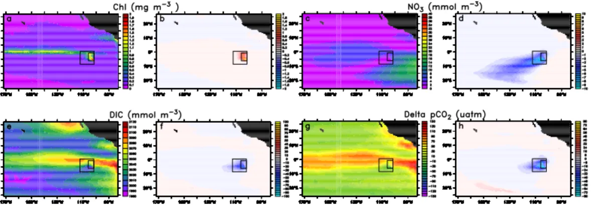
The model reproduces the observed annual-mean large-scale patterns of surface chlorophyll derived from SeaWiFS imagery reasonably well (Fig.1a and c). In fact, compared to the global-scale results of Moore et al. (2004), our Pacific-only model at eddy-permitting resolution yields somewhat higher levels of agreement, particularly

10

with regard to resolving aspects of the elevated productivity in the coastal upwelling regions along the western margin of the Americas. Perhaps the most important de-ficiency is found in the central equatorial Pacific, where the model simulates annual mean chlorophyll concentrations that are two to three times higher than those ob-served. A more quantitative assessment of the model’s skill is provided by Taylor

15

diagrams (Taylor,2001) (Fig.10a).

Similar strengths and deficiencies of the model are found for surface nitrate (Fig.1b and d). The model is successful in simulating the broad characteristics of the annual mean surface nitrate distribution synthesized from shipboard measurements (Conkright

et al.,2002), but there are a couple of notable differences. In most areas of the

sub-20

arctic North Pacific, the model’s surface nitrate concentrations are too low and model values are higher near the Bering Sea boundary, while in the eastern tropical Pacific away from the equator, the tongue of elevated nitrate extends much further southward than seen in the observations. The generally good agreement of model simulated and observed annual mean nitrate concentration is illustrated more quantitatively by a

Tay-25

lor diagram (Fig.10b).

In summary, ROMS-BEC is rather successful in modeling the main biogeochemical characteristics of the Pacific, with low nutrient/low chlorophyll, i.e. oligotrophic, condi-tions characterizing the subtropical gyres, and with HNLC condicondi-tions prevailing in the

BGD

Full Screen / Esc

Printer-friendly Version

Interactive Discussion eastern tropical Pacific and in part in the high latitudes of the North Pacific. The

de-ficiencies in the model are most likely due to the interaction of biases in the model physics with errors in the ecosystem/biogeochemical model (See Appendix C for de-tails).

The mismatches in the subarctic and tropical Pacific are clear deficiencies of our

5

model and some of the errors, for example, errors in the model length-scale of particle remineralization, ventilation time-scale of tropical thermocline, subsurface nutrient and iron fields, and iron scavenging rates, might have some impacts on our results. Be-cause our primary focus is on the atmospheric uptake efficiency, which is not expected to be sensitive to spatial mismatches in the model vis- `a-vis observations, we expect the

10

impacts are not substantial. In fact, the somewhat overly broad HNLC conditions in the eastern tropical Pacific make the iron fertilization experiments actually less sensitive to our choice of location and provide for the necessary background to undertake a wide range of experiments. In addition, we also notice the errors in the base state, for exam-ple, errors in the model length-scale of particle remineralization, ventilation time-scale

15

of tropical thermocline subsurface nutrient and iron fields, might impact our results.

4 Results

4.1 Effects of Fertilization

In the standard case, the addition of iron for 10 years to the eastern tropical Pacific induces a strong and persistent phytoplankton bloom with chlorophyll levels reaching

20

2 mg Chl m−3(Fig.2a,b), representing a roughly fivefold increase in surface chlorophyll. Inside the fertilized patch, depth integrated net primary production (NPP) is enhanced by up to 25 mol C m−2 yr−1, which corresponds to a roughly 30% increase relative to the unperturbed case (Fig.3a,b). Surface nitrate becomes depleted (Fig. 2c,d), and the reduction of surface ocean DIC by more than 30 mmol m−3 _{(Fig. 2e,f) leads to} 25

a drop in pCO2 of more than 40µatm (Fig. 2g,h). This reduction turns part of the

BGD

Full Screen / Esc

Printer-friendly Version

Interactive Discussion fertilized area, which is normally a strong source of CO₂ to the atmosphere, into a

sink (Fig.3e,f). The magnitude of the changes in NPP, chlorophyll, DIC, nitrate, and pCO2 are comparable to those observed during the most successful iron fertilization

experiments (see e.g.de Baar et al.(2005) for a summary).

After 10 years, the impact of the iron addition extends far beyond the fertilized patch.

5

This is particularly evident for surface nitrate (Fig.2c,d), where the depletion induced near the fertilization site leads to reduced nitrate concentrations downstream extend-ing for several thousand kilometers in southwesterly direction. But also the region of anomalous low pCO2 and thus anomalous uptake of CO2 from the atmosphere

(Fig.3e,f) extends over an area that is more than 5 times larger than the actually

fer-10

tilized patch. One mechanism is simply the horizontal spreading of the added iron, leading to enhanced phytoplankton production well beyond the fertilization site. How-ever, as evident from the chlorophyll changes (Fig. 2b), which extend only perhaps twofold outside the fertilized patch, this mechanism can explain only a part of the large extent of the region that is characterized by substantial pCO2 reductions. The more 15

important mechanism is the relatively slow kinetics of the exchange of CO2across the

air-sea interface. Given an equilibration time scale for the exchange of CO₂ across the air-sea interface of several months Sarmiento et al. (2007)1, surface waters that contain anomalously low pCO2 can be laterally spread for several additional months

beyond the region of elevated production before the CO₂ deficiency is removed by

20

uptake from the atmosphere.

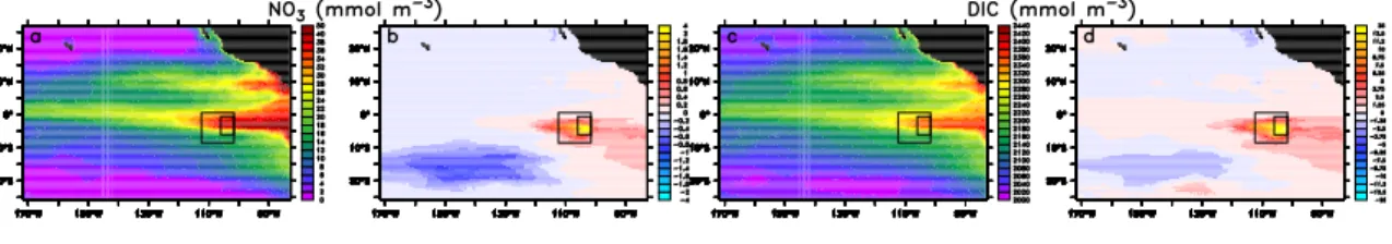
The vertical extent of the phytoplankton bloom and its associated decreases in nitrate and DIC remains limited to the mixed layer, which is between only about 15 to 40 m deep in the fertilized region. Below the mixed layer, nitrate and DIC increase relative to the unperturbed case (Fig.4), due to the remineralization of the extra organic matter

25

that is sinking through the water column. Despite a substantial amount of shallow remineralization, roughly 10% of the fertilization induced enhancement of NPP within the fertilized patch is exported as particulate organic carbon to depths below 75 m (Fig.3c,d).

BGD

Full Screen / Esc

Printer-friendly Version

Interactive Discussion The horizontal spreading of the fertilization induced perturbations in tracer

distribu-tions is even more extensive at depth than at the surface (Fig.4). At 50 m depth, the changes in DIC and nitrate are characterized by concentration increases extending from the fertilization patch far toward the east, and by a region of decreased concen-tration southwest of the patch. The former is caused by the horizontal advection of the

5

nitrate and DIC that has accumulated underneath the fertilized region, while the latter is caused by the reduction in productivity that occurred downstream (for surface flow) of the fertilized site (Fig.3b) due to the depletion in surface nitrate (Fig.2c,d).

4.2 Temporal changes

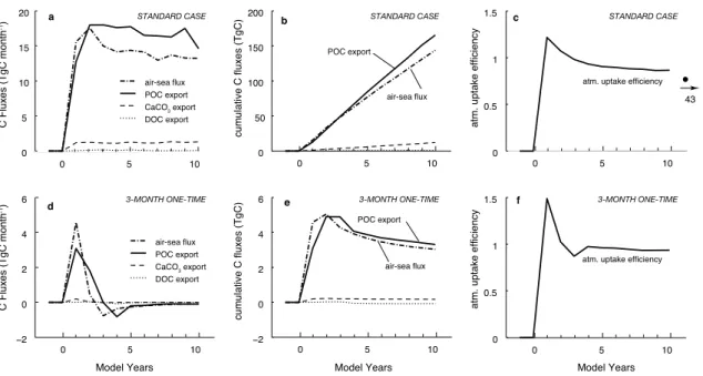
The areally integrated anomalous fluxes for the standard case (Fig.5a) show a very

10

rapid initial rise in response to the start of the iron fertilization, reaching a maximum near year 2. Thereafter, the fluxes remain essentially flat or decline gradually. The anomalous export fluxes of CaCO3 and dissolved organic carbon (DOC) are much

smaller than those for particulate organic carbon (POC), so that the POC export flux essentially determines the uptake efficiency.

15

Over 10 years, the continuous fertilization of the standard patch results in the removal of about 0.15 Pg C from the atmosphere (Table2), which corresponds to a reduction in atmospheric CO₂ of only 0.07 ppm. This cumulative uptake is driven by an iron fertilization induced export of POC, DOC, and CaCO3, which together amount to about

0.18 Pg C over 10 years. The ratio of these two cumulative fluxes is the atmospheric

20

uptake efficiency, which turns out to be 0.81 for the standard case after 10 years. Figure5c shows that for this case of continuous fertilization, the efficiency is relatively stable after 10 years, since both the air-sea CO2flux and the carbon export fluxes tend

to decrease at similar rates. Therefore, we do not expect that longer integrations of the model will substantially alter the conclusions found here. We tested this assumption

25

by continuing the iron fertilization in the STANDARD model for another 33 years for a total of 43 years. Over the course of these 33 years, the atmospheric uptake efficiency decreased only from 0.81 to 0.72, consistent with our expectation.

BGD

Full Screen / Esc

Printer-friendly Version

Interactive Discussion The time evolution of the carbon fluxes for the one-time fertilization (3MON-onetime)

is fundamentally different (Fig. 5d). Although enhanced export of POC persists for nearly three years beyond the end of the addition of iron to the system, the subsequent years (4 through 10) are characterized by smaller than normal export production. The persistence of the enhanced export is due to the fact that a substantial fraction of

5

the added iron remains in the upper ocean and is only slowly removed. However, after a few years, the slowly diminishing enhanced iron concentrations as well as the now diminished near surface concentration of macronutrients (such as nitrate) lead to a substantial reduction of export production, which takes more than 10 years to recover. The anomalous uptake of CO₂ from the atmosphere stops faster than the

10

enhanced export. Despite POC export remaining elevated, the ocean starts to lose some of the gained CO2 in year 3 and continues to do so for the rest of the 10 year

simulation. These distinct temporal changes in the carbon fluxes result in a peak in the cumulative plots in year 2 and 3, respectively (Fig.5e) and decreasing trends thereafter. Since the anomalous uptake of atmospheric CO2 peaks faster and earlier than the 15

anomalous downward export of carbon, the atmospheric uptake efficiency in this one-time fertilization has a distinct maximum in year 1 and decreases thereafter. However, since the cumulative fluxes of both air-sea exchange and vertical export decrease at a similar rate after year 3, the atmospheric uptake efficiency remains relatively constant thereafter.

20

The temporal evolution of the fluxes in the one-time case has implications for the different definitions of the atmospheric uptake efficiency. For example,Gnanadesikan

et al. (2003) defined the atmospheric uptake efficiency as the ratio of the anomalous air-sea CO2 flux integrated over the entire duration of the simulation and the

anoma-lous POC export integrated over the duration of the iron fertilization only, i.e. they used

25

different integration periods for the two fluxes. In our 3MON-onetime case, this defini-tion would not take into account the substantial addidefini-tional export of POC that occurs after the end of the fertilization, but it also would not take into account the decrease in POC export that occurs from year 3 onward. Over 10 years, Gnanadesikan’s

def-BGD

Full Screen / Esc

Printer-friendly Version

Interactive Discussion inition would yield an uptake efficiency of 1.60 for the 3MON-onetime case, which is

much higher than what our definition of the atmospheric uptake efficiency yields (0.89) (see Table 2), representing the substantial net POC export that occurs after the end of the fertilization. In our 3MON-onetime case, the iron added into the ocean is still in the surface and plays a role in the iron fertilization for some time. A better estimate

5

of anomalous POC export corresponding to Gnanadesikan’s definition is to integrate it before it becomes negative (about 3 years). This produces an efficiency of 0.60. Since we fertilize (nearly) continuously for 10 years in all other cases, the different definitions have little impact on the results (Table2).

4.3 Atmospheric uptake efficiencies

10

We compute the atmospheric uptake efficiency from the ratio of the areally and tempo-rally integrated fluxes, thus,

euptake= R a R t∆Φ CO₂ air−sead a d t R a R t∆Φ Corg+CaCO₃ export d a d t , (1) where ∆ΦCO2

air−seais the change in the air-sea CO2flux in the fertilized case in

compari-son to the unfertilized case, and ∆ΦCorg+CaCO3

export is the change in the export of biogenic

15

carbon from the euphotic zone (assumed to be 100 m deep), consisting of the export of organic carbon in both particulate (POC) and dissolved forms (DOC), and mineral CaCO₃. The perturbation fluxes are integrated in time from the beginning of the fer-tilization until time t and over the surface area a, in our case chosen as the entire

domain of our Pacific model. The atmospheric uptake efficiency for our standard

ex-20

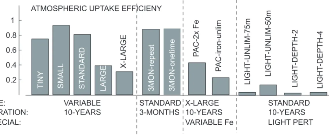
periment amounts to 0.81, with the sensitivity experiments revealing that this efficiency has large variation range with different fertilized regions, but only slightly on the dura-tion (see Fig.6, and Table2). The difference between the most efficient (SMALL with an area of 92×103km2 and euptake = 0.93) and the least efficient (X-LARGE with an

BGD

Full Screen / Esc

Printer-friendly Version

Interactive Discussion area of 15×107km2 andeuptake = 0.31) is about a factor of 3. The differences will be

explored in more detail in the discussion. By contrast there is hardly a difference in the atmospheric uptake efficiency over ten years whether the experiment is undertaken continuously (STANDARD: euptake = 0.81), for 3 months every year (3MON-repeat:

euptake = 0.88), or for 3 months only once (3MON-onetime: euptake = 0.89). Also the

5

magnitude of the iron addition is only marginally important. Doubling the magnitude of the iron added from the atmosphere in the control simulation results in an increase in the efficiency (0.43 in PAC-2xFe versus 0.31 in X-LARGE), while the addition of iron un-til phytoplankton becomes iron unlimited leads to a decrease (0.23 in PAC iron-unlim). Our range of atmospheric uptake efficiencies is similar to the values of 0.44 to

10

0.57 we infer from the recent global-scale iron flux sensitivity experiments by Moore

et al. (2006). Thus, iron fertilization experiments that actually model the addition of iron explicitly are finding atmospheric uptake efficiencies that are consistently larger than those determined earlier, using a nutrient restoring approach (e.g.,

Gnanade-sikan et al., 2003). As discussed above, the different definitions cannot explain the

15

differences, because the contribution of the non-POC export fluxes are small, and be-cause the different time-integrations also have relatively little impact over ten years for experiments with on-going fertilization.

Another issue to consider is the area over which the fluxes are integrated. As shown in Table 2, the efficiencies are generally by 20% larger if the area used is only

re-20

gional, i.e. is limited to the near-field of the patch. This is because the contribution of the anomalous outgassing far downstream of the patch is larger than the anomalous reduction of export production in the far-field. Limiting the integration to the actual fer-tilized patch yields the efficiencies that are mostly smaller than either global or regional efficiencies. This is primarily a consequence of the region of anomalous uptake of CO2 25

from the atmosphere being much larger than the patch itself, and also extending more broadly than the region of anomalous export (cf. Fig.3). Qualitatively, the sensitivity of uptake efficiency to changing integration area is similar to that found byGnanadesikan

BGD

Full Screen / Esc

Printer-friendly Version

Interactive Discussion et al. (2003) reported a factor of three difference in the efficiency depending on whether

the efficiency was determined regionally or globally. Given all these differences, it be-hooves us to understand the processes that determine the uptake efficiency.

5 Discussion

As listed in the introduction, several factors control the magnitude of the atmospheric

5

uptake efficiency: (i) The extent to which lateral and vertical transport of DIC, rather than uptake of CO₂from the atmosphere, replaces the inorganic carbon that has been taken up by the fertilized phytoplankton, converted to organic carbon, and subsequently exported to depth. By definition, the higher the fraction of carbon that comes from the atmosphere, the larger is the atmospheric uptake efficiency. (ii) The extent to which

10

the production and export of CaCO₃is stimulated. Since the formation of CaCO₃ liber-ates an aqueous CO2molecule, this process will cause outgassing to the atmosphere

(Zeebe and Archer,2005;Millero,2007;Sarmiento and Gruber,2006). Therefore, any iron fertilization induced stimulation of CaCO₃production and export would tend to re-duce the atmospheric uptake efficiency. (iii) The extent of the changes in pCO2 due 15

to the carbonate system buffering. (iv) The extent to which the outgassing CO2 from

the surface ocean in response to the lowered atmospheric CO₂ reduces the net gain of CO2 from the atmosphere. An additional factor that needs to be considered is the

timescale under consideration, and the duration of the fertilization.

The compensatory outgassing (iv) can be ruled out immediately as an explanation

20

for the large differences in the atmospheric uptake efficiencies between the different sensitivity cases considered here, since our simulations were undertaken with a fixed atmospheric pCO₂. However, the compensatory efflux can explain part of the difference between our high uptake efficiencies and the low ones reported by e.g.Gnanadesikan

et al. (2003). However, Sarmiento et al. (2007)1 shows that the consideration of a

25

variable atmospheric CO₂ results only in a 20% reduction of the atmospheric uptake efficiency over 10 years, i.e. in our standard case, the efficiency would drop from 0.81

BGD

Full Screen / Esc

Printer-friendly Version

Interactive Discussion to 0.65. Though important, this cannot close the gap between our high efficiencies and

the lower ones found in the previous nutrient-restoring based studies. The buffering effect of the ocean’s carbonate system (iii) is also not responsible for the differences, since the carbonate chemistry between the different models and sensitivity cases is nearly the same. The CaCO₃mechanism (ii) can be ruled out as well, since the

stim-5

ulation of CaCO3production and export is relatively modest in our simulations (Fig.5),

and does not change much between the different cases considered. It also cannot explain the difference to Gnanadesikan et al. (2003) since their definition, which is based on the vertical export of POC alone, actually leads to higher efficiencies (see row EFFdeplin Table2). This essentially leaves the first mechanism, i.e. lateral/vertical 10

supply versus atmospheric uptake of CO₂ as the primary explanation for the differ-ences.

The lateral/vertical supply mechanism hypothesis creates some puzzles, however, as one initially would expect the atmospheric uptake efficiency to increase as the size of the fertilized region gets larger, exactly the opposite from what we found in our

sim-15

ulations. This expectation is based on the argument that the likelihood of an inorganic carbon atom to be supplied laterally into the fertilized region to replace an atom that has been taken up by phytoplankton and exported to depth will decrease as the fer-tilized region gets larger, because the lateral area that encloses the ferfer-tilized region decreases rapidly relative to its volume. In contrast, the ratio of the area of the air-sea

20

interface relative to the volume of the fertilized region stays roughly the same, so that the likelihood of a CO2molecule to come from the atmosphere is roughly independent

of the area of the fertilized region. Putting these two trends together, one would ex-pect the atmospheric uptake efficiency to increase with increasing size of the fertilized region.

25

The answer to the puzzle and to the discrepancies with previous low efficiencies lie in the vertical distribution of the changes, as the above argument is implicitly based on the assumption that the DIC changes induced by the fertilization extend from the sur-face down to the bottom of the euphotic zone, i.e. down to 100 m. However, as noted

BGD

Full Screen / Esc

Printer-friendly Version

Interactive Discussion above, in our model iron fertilization induces a very shallow bloom, so that nutrients

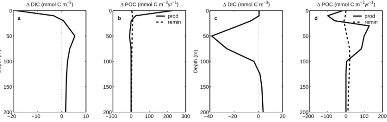
and inorganic carbon are removed only in the near-surface layers (Fig.2). Most of this carbon is not moved to great depths, but actually accumulates right underneath the surface layer, still well within the euphotic zone (Fig.4). This is illustrated in more detail in Fig.7a, which shows that, when averaged over our eastern tropical Pacific analysis

5

region (101.6◦W to 112.4◦W and 8.5 ◦S to 0.6 ◦N with an area of 7.6×105km2), DIC is depleted down to only 15 m, and that below this depth, DIC is actually elevated with a maximum just below 50 m. Analysis of the POC term balance in this region demon-strates that the rapid decrease of the net community production of POC (production minus respiration) with depth is the main cause of this strong vertical separation within

10

the euphotic zone (Fig.7b). Production of POC is enhanced just for the upper 20 m, while below this depth, the anomalous in POC production are negative in the fertilized case relative to the control run. In contrast, the remineralization of POC is enhanced throughout all depths. This leads to the net balance of POC being positive (positive net community production) for only the top 15 m, while the net balance is negative

15

(negative net community production) from 15 m downward to more than 200 m.

With most of the DIC drawdown occurring near the surface rather than near the bottom of the euphotic zone, the likelihood of the removed DIC molecule to be replaced from the atmosphere is very high. Furthermore, only a fraction of the net production of organic matter that caused the near surface drawdown of DIC is actually exported

20

below 100 m, elevating the atmospheric uptake efficiency as well. Therefore the high efficiencies in the tropical Pacific region are partly related to the low mixed layer depth there. The situations in other HNLC systems (N. Pacific, Southern Ocean), where the winter mixed layer depth matches or exceeds the euphotic depth, might be different. In fact, the low efficiency of the “whole Pacific” experiments, X-LARGE, might include

25

this impact. In addition, the X-Large experiment would also stimulate nitrogen fixation (Moore et al.,2006).

In order to assess this interpretation in more detail, we constructed a carbon budget for our eastern tropical Pacific analysis region, separating the upper ocean into a

BGD

Full Screen / Esc

Printer-friendly Version

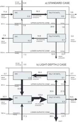
Interactive Discussion surface part (0–20 m) and a deeper part (20–100 m) of the euphotic zone (Fig. 8a).

In our standard case, the iron fertilization stimulates an increase of net community production by 31.1 TgC yr−1, and of CaCO3production by 1.1 TgC yr−1. The

corre-sponding DIC drawdown is compensated by uptake from the atmosphere (12.8 TgC yr−1_{, 40%), horizontal transport (11.9 TgC yr}−1_{, 37%), and vertical mixing and} trans-5

port from below (7.8 TgC yr−1, 23%), respectively. Three quarters of the anomalous net community production is exported vertically below 20 m, with the remaining 25% being exported horizontally. Of the 24.6 TgC yr−1_{of carbon arriving from above in the}

lower part of the euphotic zone from 20 m to 100 m, the majority (55%) is remineral-ized, leaving only 12.8 TgC yr−1for export below 100 m (11.7 TgC yr−1as POC, 1.1

10

TgC yr−1_{as CaCO}

3). Thus of the carbon exported from the top 20 m, only 48% comes

from the atmosphere, while of the carbon exported from the entire euphotic zone, more than 100% comes from the atmosphere (see regional efficiency,eregional_uptake in Table2).

This budget analysis supports our interpretation of why we get relatively high at-mospheric uptake efficiencies: First, all of the export is stimulated in the near-surface

15

layer, where the chance for a carbon atom to come from the atmosphere is much higher. Second, a high fraction of the carbon that is exported from the near surface layer remineralizes above 100 m, so that only a limited fraction continues to be ex-ported across the 100 m horizon. It appears that this effect of shallow remineralization on the magnitude of the export flux across the 100 m horizon is more important with

20

respect to atmospheric CO2uptake than the higher tendency of shallowly sequestered

carbon to escape back to the atmosphere. An important reason for the apparently small loss rates of this shallowly sequestered carbon is the relatively good retention of the added iron. If iron is retained, it will stimulate productivity when water surfaces and counter effect of elevated DIC (see Appendix D for details).

25

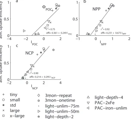
Our depth distribution hypothesis not only explains the high atmospheric uptake ficiency of our STANDARD case, but predicts successfully also the variations in ef-ficiency among our sensitivity cases (Fig. 9). More than 90% of the variance in the atmospheric uptake efficiency can be explained linearly by various indices,IP, that

ex-BGD

Full Screen / Esc

Printer-friendly Version

Interactive Discussion press how much of the fertilization induced changes across the entire euphotic zone

occur in the near-surface layer. These indices are defined as

I_P= R a Rz_ul z=0∆P d a d z R a Rz_euph z=0 ∆P d a d z (2)

wherez_ul is the depth of the upper part of the euphotic zone (here taken as 10 m), and zeuph is the depth of the euphotic zone (here taken uniformly as 100 m). The

indices are integrated over the area, a, that we used to calculate the atmospheric

5

uptake efficiency, i.e. the entire domain of our Pacific model. The expression ∆P is the

change in a particular property between the fertilization simulation and the control run. ForP , we considered the production of organic carbon (net primary production, NPP),

net community production (NCP), and the export flux of POC contributed from the layer (the differences between the bottom and top of the layer), Φ_POC. If the fertilization

10

induced changes are distributed homogeneously across the euphotic zone, IP would

have a value of 0.1. Values above this indicate a distribution skewed toward the surface, while values below this indicate a distribution skewed toward the lower part of the euphotic zone. All three measures, i.e.INPP,INCP, andIΦ_POC yield very similarr

2

, albeit slightly different linear regression equations (Fig.9).

15

The largely explained variance thus suggests that the reason for the large changes in atmospheric uptake efficiencies with the different fertilized regions is that an increas-ing fraction of the total changes occur deeper in the euphotic zone and are no longer nearly exclusively restricted to the very near surface layer. These differences in depth distribution are owing to a number of processes, including deeper mixed layers and

20

altered interaction between iron, light, and macronutrient limitation (e.g. Fe fertiliza-tion in regions with near-surface macronutrient limitafertiliza-tion will stimulate phytoplankton production further down in the water column).

In order to further explore and test our hypothesis about the depth distribution of the stimulated export production controlling the atmospheric uptake efficiency, we analyze

25

BGD

Full Screen / Esc

Printer-friendly Version

Interactive Discussion the light manipulation experiments (see Table1). In all cases, the relief from light

limi-tation results in a bloom that extends deep into the euphotic zone, causing, in the case of the LIGHT-DEPTH-2, a DIC depletion down to more than 100 m (Fig.7c). The depth changes of POC production and remineralization (Fig.7d) show enhanced growth in the lower parts of the euphotic zone, while POC production is actually reduced above

5

25 m. This is primarily due to the consumption of the macronutrients in the lower part of the euphotic zone, preventing these nutrients reaching the upper part of the euphotic zone. This effect is only partially reflected in the anomalous DIC profile (Fig.7c), since the reduced biological consumption of DIC in the upper part of the euphotic zone is nearly offset by the reduced upward transport of DIC.

10

The carbon budget of the LIGHT-DEPTH-2 case illustrates the entirely different car-bon dynamics of this deep phytoplankton bloom (Fig.8b). Net community production in the upper 20 m decreases quite substantially, causing a reduction in the organic and inorganic carbon exported from this layer (this is equivalent to an anomalous upward transport of biogenic carbon). In contrast, net community production is strongly

stim-15

ulated in the lower part of the euphotic zone, so that all of the vertical export of 55.3 TgC yr−1_{across 100 m comes from this zone. Another 15 TgC yr}−1_{is exported}

lat-erally. This exported carbon is primarily replaced by lateral transport and by reduced mixing losses to the upper part of the euphotic zone, with some additional supply from below. The net effect on the air-sea exchange within the tropical Pacific analysis region

20

is actually an anomalous outgassing, leading to a negative regional uptake efficiency. Outside the analysis region, the net effect is an anomalous uptake of CO2, but the

mag-nitude of this uptake flux is small, so that the global atmospheric uptake efficiency is only 0.04 (Table2and Fig. 6). Similarly low atmospheric uptake efficiencies are found for the other three light manipulation experiments with the exception of the

LIGHT-25

UNLIM-50 m case, which has an atmospheric uptake efficiency of 0.14. However, this value is still smaller than that of any other simulation we have undertaken (Table2and Fig.6). Although only approximately equivalent to the nutrient restoring approach used by most previous studies (Peng and Broecker,1991;Joos et al.,1991;Sarmiento and

BGD

Full Screen / Esc

Printer-friendly Version

Interactive Discussion Orr,1991;Jin and Gruber,2003;Gnanadesikan et al.,2003), these light manipulation

simulations nevertheless suggest that perhaps the most important reason for the low atmospheric uptake efficiencies identified in these previous studies is the fact that their simulation setup tended to induce export stimulation in the deep parts of the euphotic zone.

5

We thus conclude that the depth distribution of the changes in the biological pump is the key factor determining the atmospheric uptake efficiency.

6 Summary and Conclusions

The amount of CO2taken up from the atmosphere for a given change in the export of

carbon by the ocean’s biological pump, the atmospheric uptake efficiency, can vary by

10

orders of magnitude. Our experiments have shown that we can explain a very large fraction of this variance in the atmospheric uptake efficiency by considering the depth distribution of the changes in the biological pump within the euphotic zone. The higher up in the euphotic zone the biological pump is altered, the higher is the likelihood that an exported carbon atom comes from the atmosphere, i.e. the higher is the atmospheric

15

uptake efficiency. Iron fertilization of near surface waters tends to induce very shallow blooms and export production, resulting in high atmospheric uptake efficiencies. The response is independent of the source of the additional near-surface iron input, which could come from the atmosphere, deliberate iron injection or shallow sediments. Al-though the efficiency is high, the total amount of carbon that can be taken out of the

20

atmosphere by iron fertilization is small. Even in the case of fertilization of the entire North and Tropical Pacific, the total air-sea flux over 10 years is only 3.4 Pg C. This supports the results of other iron fertilization experiments that also show small poten-tial for changes in atmospheric iron supply to alter atmospheric CO2(e.g.,Aumont and

Bopp,2006;Bopp et al.,2003;Moore et al.,2006).

25

Our findings have important implications for understanding and predicting the impact of changes in the biological pump on atmospheric CO2. Although we have used

BGD

Full Screen / Esc

Printer-friendly Version

Interactive Discussion marily iron addition experiments as our tool to induce changes in the biological pump,

the importance of the depth distribution in controlling the impact on atmospheric CO₂ of changes in the biological pump is largely independent of the actual mechanism that causes this change. Therefore, studies that investigate the impact of past or future changes in the biological pump on atmospheric CO₂ need to consider not only the

5

changes in the export flux across the bottom of the euphotic zone, but also where within the euphotic zone the biological changes occur. A corollary to this is the need for modelers to pay more attention to the details of upper ocean physics and ecol-ogy/biogeochemistry in their models (Doney,1999).

Appendix A The efficiency of iron fertilization

10

A measure of the overall impact of the addition of iron on atmospheric CO₂ is the carbon-to-iron fertilization ratio, which describes how much additional CO2is taken up

from the atmosphere for a given amount of iron added to the ocean (c.f. Sarmiento et al. (2007)1): R_fertC:Fe= R a R t∆Φ CO₂ air−sead a d t R a R t∆Φ Fe fertd a d t , (A1) where ∆ΦCO2

air−sea is the change in the air-sea CO2 flux in the fertilized case in

com-15

parison to the unfertilized case, and ∆ΦFe_fert is the iron flux added to the ocean. The perturbation fluxes are integrated in time from the beginning of the fertilization until timet and over the surface area a, usually chosen as the global surface ocean or in

the case of regional models the entire model domain. Assuming that this fertilization ratio can be estimated well for any size and duration of experiment, knowledge of its

20

value would then permit to predict the net air-sea CO2flux that would result from any

BGD

Full Screen / Esc

Printer-friendly Version

Interactive Discussion Since the process driving the perturbation in the air-sea CO₂flux is the iron induced

change in the biological export of carbon from the near surface ocean (euphotic zone), it is instructive to split the fertilization ratio into an efficiency part that reflects how much CO₂is taken up from the atmosphere per unit change in biological export (termed the atmospheric uptake efficiency, euptake), and into a biological iron utilization ratio that 5

reflects how a given amount of added iron stimulates the biological export of carbon (termed the iron utilization ratio,R_{iron util}C:Fe ), thus:

e_uptake= R a R t∆Φ CO₂ air−sead a d t R a R t∆Φ C_org+CaCO₃ export d a d t , (A2)

R_{iron util}C:Fe =

R a R t∆Φ C_org+CaCO3 export d a d t R a R t∆Φ Fe fertd a d t , (A3)

where ∆ΦC_exportorg+CaCO3 is the change in the biologically mediated export of carbon from

10

the euphotic zone (assumed to be 100 m deep), consisting of the export of organic carbon in both particulate (POC) and dissolved forms (DOC), and mineral CaCO3.

By definition, the product of the atmospheric uptake efficiency and the biological iron utilization ratio is the fertilization ratio:

R_fertC:Fe=_{euptake· R}C:Fe

iron util. (A4)

The atmospheric CO2 uptake efficiency describes how the inorganic carbon that is 15

lost to depth by the iron fertilization induced stimulation of biological export is replaced (see the discussion in the section introduction). The iron utilization ratio describes how iron added to the ocean stimulates the export of biological carbon. The value of this ratio depends on very complex processes, involving iron chemistry, especially the de-gree to which iron is scavenged from the water column relative to carbon and nutrients,

20

BGD

Full Screen / Esc

Printer-friendly Version

Interactive Discussion phytoplankton metabolism, food web cycling, and the interaction of aphotic iron

chem-istry with large-scale ocean circulation and mixing (see Sarmiento et al. (2007)1for a more detailed discussion).

Appendix B Taylor diagrams

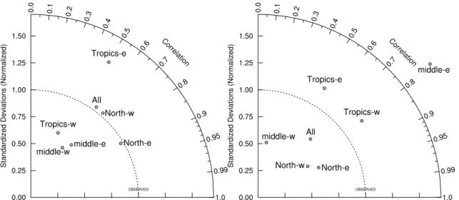
A more quantitative assessment of the model’s skill is provided by Taylor diagrams

5

(Taylor, 2001) (Fig. 10a). These diagrams illustrate the level of agreement between the model and the observations in polar coordinates, with the correlation shown as the angle from the vertical in clockwise direction, and with the standard deviation of the modeled field relative to that of the observations shown as the distance from the origin. In such a diagram, the distance between the resulting end point and the point

10

located on the abscissa at a relative standard deviation of 1 (representing a perfect match) is the root mean square (RMS) error of the model with regard to a particular set of observations. The correlation of annual mean chlorophyll between the model and the SeaWiFS derived observations for the entire Pacific north of 10◦_{S is a respectable}

0.60. The model’s standard deviation of that pattern is nearly identical to that of the

15

observations, giving a relative standard deviation of about 1. Splitting the model do-main into sub-regions reveals that the level of agreement varies substantially within the Pacific. The lowest RMS error is found for the eastern North Pacific (>30◦_{N, and east}

of 166◦W), while the eastern tropical Pacific (10◦S to 10◦N, and east of 166◦W) has the highest RMS error. The latter is largely due to the overestimation of chlorophyll by the

20

model near the equator while the concentrations off the equator are similar, causing a much higher standard deviation in the model results compared to the observations.

The generally good agreement of model simulated and observed annual mean nitrate concentration is also illustrated more quantitatively by the Taylor diagram (Fig.10b) (correlation of nearly 0.67, although with a standard deviation that is slightly

25

lower than observed). As was the case for chlorophyll, analyses of the agreement be-tween model results for nitrate and observations show large differences for the different