HAL Id: hal-00001445
https://hal.archives-ouvertes.fr/hal-00001445v2
Submitted on 14 Apr 2004
HAL is a multi-disciplinary open access
archive for the deposit and dissemination of
sci-entific research documents, whether they are
pub-lished or not. The documents may come from
teaching and research institutions in France or
abroad, or from public or private research centers.
L’archive ouverte pluridisciplinaire HAL, est
destinée au dépôt et à la diffusion de documents
scientifiques de niveau recherche, publiés ou non,
émanant des établissements d’enseignement et de
recherche français ou étrangers, des laboratoires
publics ou privés.
Resetting chemical clocks of hot cores based on
S-bearing molecules
Valentine Wakelam, Paola Caselli, Cecilia Ceccarelli, Eric Herbst, Alain
Castets
To cite this version:
Valentine Wakelam, Paola Caselli, Cecilia Ceccarelli, Eric Herbst, Alain Castets. Resetting chemical
clocks of hot cores based on S-bearing molecules. Astronomy and Astrophysics - A&A, EDP Sciences,
2004, 422, pp.159. �10.1051/0004-6361:20047186�. �hal-00001445v2�
ccsd-00001445, version 2 - 14 Apr 2004
(DOI: will be inserted by hand later)
Resetting chemical clocks of hot cores based on
S–bearing molecules
V. Wakelam
1, P. Caselli
2, C. Ceccarelli
3, E. Herbst
4and A. Castets
11 Observatoire de Bordeaux, BP 89, 33270 Floirac, France 2
INAF–Osservatorio Astrofisico di Arcetri, Largo E. Fermi 5, 50125 Firenze, Italy
3
Laboratoire d’Astrophysique, Observatoire de Grenoble - BP 53, F-38041 Grenoble cedex 09, France
4
Departments of Physics, Chemistry, and Astronomy, The Ohio State University, Columbus, OH 43210, USA
Received April 14, 2004 ; accepted
Abstract. We report a theoretical study of sulphur chemistry, as applied to hot cores, where S-bearing molecular ratios have been previously proposed and used as chemical clocks. As in previous models, we follow the S-bearing molecular com-position after the injection of grain mantle components into the gas phase. For this study, we developed a time-dependent chemical model with up-to-date re-action rate coefficients. We ran several cases, using different realistic chemical compositions for the grain mantles and for the gas prior to mantle evaporation. The modeling shows that S-bearing molecular ratios depend very critically on the gas temperature and density, the abundance of atomic oxygen, and, most im-portantly, on the form of sulphur injected in the gas phase, which is very poorly known. Consequently, ratios of S-bearing molecules cannot be easily used as chem-ical clocks. However, detailed observations and careful modeling of both physchem-ical and chemical structure can give hints on the source age and constrain the mantle composition (i.e. the form of sulphur in cold molecular clouds) and, thus, help to solve the mystery of the sulphur depletion. We analyse in detail the cases of Orion and IRAS16293-2422. The comparison of the available observations with our model suggests that the majority of sulphur released from the mantles is mainly in, or soon converted into, atomic form.
1. Introduction
It is a long-standing dream to use relative abundances of different molecules as chemical clocks to measure the ages of astronomical objects. Studies of the ages of star formation regions have recently focused on S-bearing molecules. Charnley (1997) and Hatchell et al. (1998) were the first to propose that the relative abundance ratios of SO, SO2 and H2S
could be used to estimate the age of the hot cores of massive protostars. The underlying idea is that the main reservoir of sulphur is H2S on grain mantles, and that when the hot
core forms, the mantles evaporate, injecting the hydrogen sulphide into the gas phase. Endothermic reactions in the hot gas convert H2S into atomic sulphur and SO from which
more SO and, subsequently, SO2 are formed, making the SO2/SO and SO/H2S ratios
nice functions of time. These studies have triggered a variety of work, both observational and theoretical (Charnley 1997; Hatchell et al. 1998; Buckle & Fuller 2003).
This line of research, however, has been challenged by recent ISO observations, which have cast doubt on the basic assumption that sulphur is mainly trapped in grain mantles as H2S. The lack of an appropriate feature in the ISO spectra of high (Gibb et al. 2000)
and low (Boogert et al. 2000) mass protostars sets an upper limit on the mantle H2S
abundance which cannot exceed about 10−7 with respect to H
2 (van Dishoeck & Blake
1998). Indeed, the identity of the major reservoir of sulphur in cold molecular clouds is a long standing and unresolved problem, for the sum of the detectable S-bearing molecules is only a very small fraction of the elemental S abundance (Tieftrunk et al. 1994). Since sulphur is known not to be depleted in the diffuse medium (e.g. Sofia et al. 1994), it is usually assumed that sulphur in dense clouds is depleted onto the grain mantles rather than in refractory cores (e.g. Caselli, Hasegawa, & Herbst 1994), but how this happens is a mystery. In a theoretical study, Ruffle et al. (1999) proposed that in collapsing translucent clouds sulphur is efficiently adsorbed onto grain mantles. In fact, in these regions, most of the gas-phase sulphur is in the form of S+, while grains are typically
negatively charged, so that the collisional cross section for sulphur is enhanced compared with neutral species (e.g. O) and sulphur is removed from the gas phase more rapidly.
Another mystery is the form of sulphur on dust grains. The simplest possibility is that it consists of relatively isolated atoms, as would occur in a matrix, or perhaps as isolated pairs of atoms (S2). Another possibility is that the sulphur is amorphous (or
even crystalline), having formed islands of material from the initially adsorbed atoms. Crystalline sulphur is known to come in two forms - rhombic and monoclinic - both of which consist of S8 cyclic molecules. Vaporization leads to a complex mixture of sulfur
polymers through S8 in complexity. If sulphur is elemental and amorphous, evaporation
is also likely to lead to molecules of sulphur through eight atoms in complexity. So far, the only S-bearing species firmly detected on granular surfaces is OCS, but with a
relatively low fractional abundance of 10−7(Palumbo et al. 1997). Recently, Keller et al.
(2002) claimed the detection of iron sulphide (FeS) grains in protoplanetary disks, but there is no evidence to suggest that solid FeS is the main form of sulphur in the parent collapsing environment. Actually, if the main form of solid sulphur is FeS, S should follow Fe depletion, which is not observed (Sofia et al. 1994). Even more recently, Scappini et al. (2003) suggested that hydrated sulphuric acid (H2SO4·H2O) is the main sulphur
reservoir. In whatever form sulphur resides in the grain mantles, there is the possibility that the species, once evaporated, are very quickly destroyed to give atomic sulphur. In summary, although all the evidence is that sulphur is depleted onto grain mantles in cold clouds, its particular form is very uncertain.
Given the need for chemical clock methods, it is timely to reconsider the use of S-bearing molecules in this fashion. In this paper, we present a model with an up-to-date chemical network involving S-bearing molecules. We run several cases to cover a large, realistic parameter space for hot core sources, consistent with present observational constraints. Based on the results we obtain, we conclude that it is tricky to use abundance ratios of S-bearing molecules as chemical clocks in the absence of other constraints, for they depend more on the initial conditions, gas density, temperature, and the initial form of sulphur injected in the gas phase than on the age of the source.
The paper is organized as follows: we describe the model in §2, the model results in §3, and in §4 we discuss the practical consequences of those results and apply the model to the specific cases of Orion and IRAS16293-2422.
2. The Model
We have developed a pseudo-time dependent model for the gas phase chemistry that computes the evolution of the chemical composition of a volume of gas with a fixed density and temperature. Our goal is to follow how the S-bearing molecular abundances vary with time when the gas undergoes a sudden change in its temperature and density, and/or in its overall chemical abundance, because of the evaporation of grain mantles. In hot cores the dust temperature increases to an extent that it exceeds the mantle evaporation temperature, i.e. ∼100 K, and all the components of the grain mantles are suddenly injected into the gas phase, similarly to what has been done in previous studies of hot cores (e.g. Brown et al. 1988; Charnley et al. 1992; Caselli et al. 1993; Millar et al. 1997b). In fact, it is more probable that hot cores have spatial gradients in temperature and density releasing the molecules at different times depending on their surface binding energies (see Ceccarelli et al. 1996; Viti & Williams 1999; Doty et al. 2002; Rodgers & Charnley 2003). However, the goal of this work is mainly to test the effects of the form of the main initial sulphur bearing molecules and we preferred to simplify the problem
assuming that all the molecules evaporate simultaneously from the grain. More detailed models will be presented in a forthcoming paper.
In order to simulate these conditions, the gas-phase chemical composition prior to evaporation of the mantles is taken to be similar to that of dark molecular clouds. At time t= 0, the grain mantle components are injected into the gas phase, and the model follows the changes in the gas chemical composition with a given gas temperature and density. Throughout this paper we will use the word “evaporation” to refer to the loss of the grain mantles.
The model is a reduced chemical network, which includes 930 reactions in-volving 77 species containing the elements H, He, C, O and S. The standard neutral-neutral and ion-neutral reactions are considered. Most of the reaction co-efficients are from the NSM (“new standard model”; http://www.physics.ohio − state.edu/ eric/research−f iles/cddata.july03) database; see also Lee, Bettens, &
Herbst (1996), updated with new values or new analyses of assorted values in databases (e.g. the NIST chemical kinetics database at http://kinetics.nist.gov/index.php) when available. Furthermore, several high temperature (neutral-neutral) reactions have been added. To select the reduced network, we have followed Ruffle et al. (2002) for CO forma-tion, Hollenbach & McKee (1979) and Hartquist et al. (1980) for the oxygen chemistry and Pineau Des Forˆets et al. (1993) and Charnley (1997) for the sulphur chemistry.
To validate this network, we compared our results with abundances previously ob-tained by Lee, Bettens, & Herbst (1996) at low temperature and Charnley (1997) at higher temperatures using the same initial abundances as these authors. We found that we can reproduce molecular abundances to better than a factor of three. This is an indication that small variations in the rate coefficients between the updated NSM and UMIST databases do not strongly influence the computed abundances of sulphur bearing species. One exception is the CS molecule, which we produce at an abundance ten times less than Charnley’s model, because our adopted rate coefficient for the reaction CO + CRPHOT → O + C, (where CRPHOT is a photon induced by cosmic rays) is 50 times smaller than in the UMIST database. The lowered abundance of C then translates into a lowered abundance for CS, since C is a precursor of CS.
Note that we have assumed the gas to be totally shielded from the interstellar UV field and no other UV field to be present. Thus, the model does not include any pho-tochemistry, with the exception of cosmic ray–induced photodestruction reactions. The model takes into account a reduced gas-grain chemistry: H2 is formed on grain surfaces
and the recombination of ions with negatively charged grains occurs (see Aikawa et al. 1999, for the recombination of ions with negative grains). Moreover, neutral species can deplete onto grain mantles, and mantle molecules can evaporate because of thermal effects and cosmic rays (Hasegawa, Herbst, & Leung 1992; Hasegawa & Herbst 1993).
2.1. Gas-phase and mantle abundances prior to evaporation
To help determine a set of molecular abundances prior to mantle evaporation, we ran the model with a temperature equal to 10 K and a density nH2 equal to 104 cm−3, including
freeze out, for 107
yr. At this time, species such as SO, SO2, and CS reach abundances
similar to those observed in dark clouds (∼ 10−9, ≤ 10−9, and ∼ 10−9, respectively;
Dickens et al. 2000). The adopted elemental abundances (with respect to H2) for He, O,
C+ and S+ are respectively: 0.28, 6.38 × 10⁻⁴ (Meyer et al. 1998), 2.8 × 10⁻⁴ (Cardelli
et al. 1996) and 0.3×10⁻⁴; the sulphur abundance refers to the gaseous and grain portions
(see below). The late-time abundances obtained could not be reasonably used without modification for the pre-evaporated chemical composition for several reasons. First, our model, like most other gas-phase treatments (e.g. Lee et al. 1996; Millar et al. 1997a), overestimates the O2and H2O abundances in cold dense clouds by orders of magnitude
with respect to the ISO, SWAS and ODIN observations (e.g. Bergin et al. 2003; Pagani et al. 2003). Secondly, the elemental sulphur abundance pertaining to the gas must be lowered to avoid getting very high abundances of sulphur-bearing species. The portion of the abundance not used for the gas can be considered to reside in grain mantles until evaporation or in grain core. In order to mimic realistic conditions, we thus adopted three different compositions for the pre-evaporative gas, as follows:
Composition A: We adopted the computed late-time molecular abundances except for O2 and H2O, which were assumed to be 10−7 and 10−8 with respect to H2 respectively,
in agreement with observations in molecular clouds , and for atomic oxygen, O, which was assumed to carry the oxygen not locked into CO, leading to a fractional abundance of 2.6 × 10⁻⁴, as suggested by observations (e.g. Baluteau et al. 1997; Caux et al. 1999;
Vastel et al. 2002; Lis et al. 2001). In addition, the initial gas-phase sulphur abundance was taken to be a factor of 30 lower than the elemental abundance.
Composition B: We re-computed the late time abundances, lowering artificially by two orders of magnitude the rate of the dissociative recombination of H3O+, to decrease
the computed O2 and H2O abundances. In this case, it was only necessary to lower the
initial elemental sulphur abundance by a factor of five. The abundance of atomic oxygen in this case is 4.8 × 10⁻⁴, consistent with observations in molecular clouds.
Composition C: The abundances were taken to equal those measured in the direction of L134N, as reported in Table 4 of Charnley, Rodgers, & Ehrenfreund (2001). The oxygen not contained in the species reported in Table 4 was assumed to be in atomic form.
All three gas-phase compositions have large abundances of atomic oxygen, in agree-ment with observations. We assume that this large O abundance is also present at the beginning of the hot core phase, in contrast with previous studies. This implies many differences in the computed abundances, as shown in Section 3.1 and discussed in Section
Table 1.Computed late time (A, B) and adopted (C) gas-phase abundances with respect to H2for the main S-bearing molecules prior to mantle evaporation.
Species A B C SO 9 × 10⁻⁹ 3 × 10⁻⁹ 3.1 × 10⁻⁹ SO2 4 × 10⁻¹⁰ 1.5 × 10⁻¹⁰ 1 × 10⁻⁹ a H2S 1 × 10⁻¹⁰ 1 × 10⁻¹¹ 8 × 10⁻¹⁰ CS 4 × 10⁻¹⁰ 2 × 10⁻⁸ 1.7 × 10⁻⁹ a
Here we took the value of the upper limit.
Table 2. Adopted abundances for mixtures of evaporated S-bearing molecules (with respect to H2).
Species Mod. 1 Mod. 2 Mod. 3 Mod. 4 OCS 10−7 10−7 10−7 10−7
H2S 10−7 10−7 10−7 10−8
S 0 3 × 10⁻⁵ 0 3 × 10⁻⁵
S2 0 0 1.5 × 10⁻⁵ 0
4.1. Table 1 lists the abundances of the main S-bearing molecules for the three gas-phase compositions prior to mantle evaporation.
At time t = 0, the grain mantle components are injected into the gas phase. The abundances of the major mantle components are relatively well constrained by the ob-servations and we took the observed abundances (with respect to H2) in high mass
pro-tostars: H2O: 10−4 (Schutte et al. 1996), H2CO: 4 × 10⁻⁶(Keane et al. 2001), CH3OH:
4 × 10⁻⁶ (Chiar et al. 1996) and CH
4: 10−6 (Boogert et al. 1998). Note that in order
to shorten the number of treated species, we negleted the CO2 molecule which is
abun-dant in mantles (2 × 10⁻⁵ with respect to H
2, Gerakines et al. 1999), because it is not
a crucial element of the sulphur chemistry. On the contrary, the situation is very uncer-tain with respect to the S-bearing mantle molecules, as discussed in the Introduction. In order to study the influence of the injected S-bearing abundances on the evolution of the chemical composition, we have run models with four types of material evaporating from mantles that differ in their major sulphur-bearing species, as reported in Table 2. In practice, sulphur on the grain mantles can be stored as OCS, H2S, or pure sulphur
in a matrix-like, amorphous, or even crystalline form. Of the four mixtures, the first one (used in Model 1) has the bulk of the sulphur in the refractory core of the grain, while the other three (used in Models 2-4) have large abundances of elemental sulphur leading upon evaporation directly or eventually to either S or S2 in the gas.
2.2. ”Important” reactions
As the post-evaporative gas-phase chemistry proceeds, it is important to determine the reactions that will influence the formation and destruction of sulphur-bearing species the most severely. We will call them ”important” reactions in the following discussion. By this term, we mean quantitatively those reactions that lead to significant variations of the main S-bearing abundances when the relevant reaction rate is changed by a small amount (specifically 10%). Although such a determination has not been featured in pa-pers on astrochemistry, we thought it worthwhile to introduce a suitable procedure here. The aim of this study is twofold: (i) to determine a set of reactions to check carefully in laboratory experiments because the computed abundances are particularly sensitive to those reactions, and (ii) to ascertain whether different chemical networks will lead to different results, and why. To identify these reactions, we first defined a “perturbation” in the rate coefficient for each of the 750 gas–phase reactions by multiplying them by a factor of 1.1, one at a time. For each single perturbation, we then computed the abun-dance “variations” ∆X by comparing the computed abunabun-dances after 104 yr with the
reference abundances calculated with the non-modified set of reaction rates, according to the expression ∆X = |Xref−X|
Xref , where Xref is the reference abundance and X the
abundance obtained with the perturbed rate.
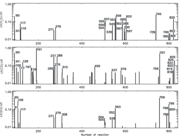
Fig 1 shows the variations of the abundances of the main S-bearing species H2S, CS,
and SO divided by the amplitude of the perturbation (∆R = 0.1) for a temperature of 100 K and a density of 107 cm−3. The calculation has been performed for composition
A and Model 2. The abscissa consists of the numbers of reactions in our network from 86 to 834. Vertical lines are included for those reactions that produce a normalized variation larger than 1% of the largest variation, while the actual numbers of reactions with a normalized variation greater than 5% are listed. Note that for a variation (0.1) equal in size to the amplitude of the perturbation, the line extends upward to unity and that a ∆X/∆R of 0.5 implies that the abundance of the studied molecule change by 5% in abundance upon a 10% change in the reaction rate. The sets of numbered “important” reactions for the molecules H2S, CS, and SO consist of 28, 24, and 17
reactions, respectively. We do not show the variations of OCS and SO2because the OCS
abundance is only affected significantly (9%) if reaction 757 is perturbed, while SO2
shows the same behavior as SO so the corresponding figure is the same.
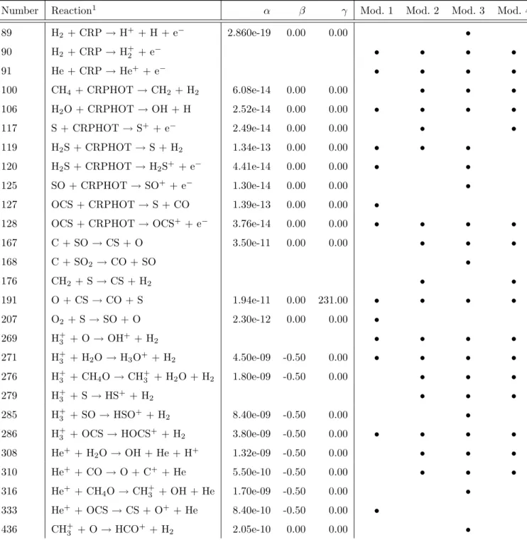
In Table 3, we list the 70 most important reactions for the chemistry of H2S, CS, SO,
SO2 and OCS for initial composition A and the four models (see previous section) at a
temperature of 100 K and a density of 107cm−3. The first two columns give the number
of the reaction and the actual reaction, while the third column gives the reaction rate coefficient k in terms of the standard parameters α (cm3 s−1), β and γ (K):
∆ X (H 2 S )/ ∆ R ∆ X (CS)/ ∆ R ∆ X (SO )/ ∆ R
Fig. 1.The “variation” ∆X (see text) of the abundances of SO, H2S, and CS divided by
the amplitude (∆R = 0.1) of the perturbation of the rate coefficients plotted for reactions with number between 86 and 834; i.e., all the reactions in the model exept those dealing with dust grains. The numbers indicate those reactions that induce a variation of more than 5% of the highest variation for each species.
where T is the gas temperature. In this table, we report only the rate coefficients that differ by more than 10% from the UMIST ones. In the last four columns, the symbol • indicates that the reaction is important for sulphur chemistry in the model of the corresponding column. The list of reactions in Table 3 depends only weakly on the choice of initial composition mentioned in section 2.1, because the three initial compositions A, B and C give sufficiently similar abundances at 104 yr.
Of course, for very different initial compositions, the list of important reactions could be slightly different, especially if the network is different. This is for example the case of the Charnley (1997) model, where all reactions involving atomic oxygen are not impor-tant, for no initial gaseous atomic oxygen is assumed to be present, whereas ion–molecule reactions involving molecular ions such as H+
3, H3O+, and H3CO+, are crucial.
We found that the relative importance of the reactions in Table 3 depends more on the initial mantle composition (Model 1 to 4) than on the pre-evaporation composition of the gas (A, B or C). For Model 1, the chemical network is simpler (i.e. fewer important reactions) than for Models 2, 3, and 4 because there is no initial S or S2, so that many
have a similar list of important reactions but some reactions with SO gain in importance for Model 3. Models 2 and 4 are even more similar in their lists of important reactions. A few reactions with H2S become less important for Model 4 because the initial abundance
of H2S in this model is ten times less than in Model 2 and only one reaction (number
550) becomes important.
Table 3: List of the reactions important for the chemistry of the SO, SO2, OCS, H2S and CS molecules for a temperature of 100 K
and a density of 107cm−3 with initial composition A.
Number Reaction1 α β γ Mod. 1 Mod. 2 Mod. 3 Mod. 4
89 H2 + CRP → H+ + H + e− 2.860e-19 0.00 0.00 • 90 H2 + CRP → H+2 + e− • • • • 91 He + CRP → He+ + e− • • • • 100 CH4 + CRPHOT → CH2+ H2 6.08e-14 0.00 0.00 • • • 106 H2O + CRPHOT → OH + H 2.52e-14 0.00 0.00 • • • • 117 S + CRPHOT → S+ + e− 2.49e-14 0.00 0.00 • • 119 H2S + CRPHOT → S + H2 1.34e-13 0.00 0.00 • • • 120 H2S + CRPHOT → H2S+ + e− 4.41e-14 0.00 0.00 • • 125 SO + CRPHOT → SO+ + e− 1.30e-14 0.00 0.00 • 127 OCS + CRPHOT → S + CO 1.39e-13 0.00 0.00 •
128 OCS + CRPHOT → OCS+ + e− 3.76e-14 0.00 0.00 • • • •
167 C + SO → CS + O 3.50e-11 0.00 0.00 • • • 168 C + SO2 →CO + SO • 176 CH2 + S → CS + H2 • • 191 O + CS → CO + S 1.94e-11 0.00 231.00 • • • • 207 O2 + S → SO + O 2.30e-12 0.00 0.00 • 269 H+3 + O → OH + + H2 • • • • 271 H+ 3 + H2O → H3O++ H2 4.50e-09 -0.50 0.00 • • • • 276 H+ 3 + CH4O → CH + 3 + H2O + H2 1.80e-09 -0.50 0.00 • • • 279 H+ 3 + S → HS + + H 2 • • • 285 H+ 3 + SO → HSO ++ H 2 8.40e-09 -0.50 0.00 • 286 H+ 3 + OCS → HOCS + + H 2 3.80e-09 -0.50 0.00 • • • • 308 He++ H 2O → OH + He + H+ 1.32e-09 -0.50 0.00 • • • 310 He++ CO → O + C+ + He 5.50e-10 -0.50 0.00 • • • 316 He+ + CH4O → CH + 3 + OH + He 1.70e-09 -0.50 0.00 • 333 He+ + OCS → CS + O+ + He 8.40e-10 -0.50 0.00 • 436 CH+3 + O → HCO + + H2 2.05e-10 0.00 0.00 •
437 CH+ 3 + O → HOC ++ H 2 • 447 CH+ 3 + SO → HOCS + + H2 4.20e-09 -0.50 0.00 • 459 CH4 + S+ →H3CS+ + H 1.40e-10 0.00 0.00 • • • 504 O + HS+ →S+ + OH • • • 505 O + HS+ →SO+ + H • • • 506 O + H2S+ →HS+ + OH • • • 507 O + H2S+ →SO+ + H2 • • • 537 H2O + HCO+→CO + H3O+ 2.10e-09 -0.50 0.00 • • • 539 H2O + HS+ →S + H3O+ • • • 540 H2O + H2S+ →HS + H3O+ 7.00e-10 0.00 0.00 • • • 550 H2O+ + H2S → H3S+ + OH 7.00e-10 0.00 0.00 • 552 H3O+ + H2CO → H3CO++ H2O 2.60e-09 -0.50 0.00 • • • • 553 H3O+ + CH4O → CH5O+ + H2O • • • • 556 H3O+ + H2S → H3S+ + H2O • • • • 579 HCO+ + OCS → HOCS+ + CO 1.50e-09 -0.50 0.00 • • • 585 H2CO + S+ →H2S+ + CO 1.10e-09 -0.50 0.00 • • • 586 H2CO + S+ →HCO++ HS 1.10e-09 -0.50 0.00 • • • 587 H2CO + H3S+ →H3CO+ + H2S • • • 595 S + H3S+ →H2S+2 + H • • 597 S+ + H 2S → S+2 + H2 6.40e-10 -0.50 0.00 • • 603 H2S + SO+ →S+2 + H2O 1.10e-09 0.00 0.00 • • • 614 H+ + H2O → H2O++ H 7.30e-09 -0.50 0.00 • 624 H+ + SO → SO+ + H 1.40e-08 -0.50 0.00 • 739 S + HS+ →HS + S+ • • 740 S + H2S+ →H2S + S+ • • • 751 H2 + CH + 3 →CH + 5 + PHOTON • 756 O + SO → SO2 + PHOTON 3.20e-16 -1.60 0.00 • • • • 757 CO + S → OCS + PHOTON • • • • 789 H3O+ + e− →OH + H + H • • 798 H3CO+ + e− →CO + H + H2 • • • 799 H3CO+ + e− →HCO + H + H • • • 800 H3CO+ + e− →H2CO + H • • 803 CH5O+ + e− →CH4O + H • • 804 CH5O+ + e− →H2CO + H2 + H • • 812 H3S+ + e− →HS + H + H 1.00e-07 -0.50 0.00 • 818 H3CS+ + e− →CS + H2 + H • • 819 H3CS+ + e− →H2CS + H • • 820 SO+ + e− →S + O • • •
821 HSO+ + e− →SO + H • 822 OCS+ + e− →CO + S 3.00e-07 0.00 0.00 • • • 823 OCS+ + e− →CS + O • • • 824 HOCS+ + e− →CS + OH • • • • 825 HOCS+ + e− →OCS + H • • • •
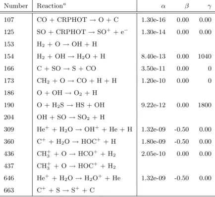
The above analysis of “important” reactions refers to only one perturbation ampli-tude. In general, since the equations are not linear, the amplitude of the perturbation may influence the results in a non-linear way. To check for non-linearity, we also ran the case where each reaction rate is twice as large as the ”standard” one (i.e. a pertubation amplitude of 1.0, which doubles the rate of reaction), and still obtained linear variations, so that normalized variations are independent of amplitude. One exception concerns CS, for which several reactions become important in the latter case. These reactions, listed in Table 4 for composition A and Model 2, must be added to the ones shown in Fig. 1 for CS.
Because rate coefficients are often dependent on the temperature, a change in this parameter can affect which reactions are important. In particular, an increase of the tem-perature to 200 K makes some of the neutral-neutral reactions more important (Table 5) and some reactions (579, 789, 798, 800, 804 and 825) of Table 3 negligible. On the con-trary, an increase of the H2density to 108cm−3 does not change the results significantly.
Finally, from Tables 3 and 5 and Fig. 1, we can determine the reactions producing the largest variations for the S-bearing species under a set of relevant conditions and a reasonable time (104 yr) for our models: reactions 90, 153, 190, 191, 740, 756 and 757.
Reaction 90 is the cosmic ray ionization rate of H2, which is obviously important for
starting the ion-molecule chemistry. Reactions 153 and 190 are neutral-neutral reactions important only at the higher temperature considered (200 K). The other reactions (cf Table 3) are a collection of ion-molecule (740), neutral-neutral (191), and radiative asso-ciation (756 and 757) processes. The importance of these reactions would probably have been overlooked had this analysis not been done. It will therefore be crucial to know the rate coefficients of the mentioned reactions with high precision. Of these reactions, only the rate coefficient for 153 is well determined in the laboratory, although the lowest measured temperature (300 K) means that the rate coefficient in the 100-200 K range involves an extrapolation. Uncertain measured activation energies for reactions 190 and 191 also lead to poorly determined rate coefficients by 100-200 K. The ion-molecule re-action (740) may not even be exothermic, while the rate coefficients for the radiative association processes are order-of-magnitude estimates at best.
Table 4.Additional important reactions for a perturbation amplitude of 1.0, for Model 2 and Composition A. Number Reactiona α β γ 168 C + SO2 →CO + SO 173 CH2 + O → CO + H + H 1.20e-10 0.00 0.00 308 He+ + H 2O → OH + He + H+ 1.32e-09 -0.50 0.00 309 He+ + H2O → OH+ + He + H 1.32e-09 -0.50 0.00 333 He+ + OCS → CS + O+ + He 8.40e-10 -0.50 0.00 360 C+ + H2O → HOC + + H 1.80e-09 -0.50 0.00 444 CH+ 3 + S → HCS + + H2 447 CH+ 3 + SO → HOCS + + H2 4.20e-09 -0.50 0.00 459 CH4 + S + →H3CS + + H 1.40e-10 0.00 0.00 509 O + HCS+ →S + HCO+ 5.00e-10 0.00 0.00 510 O + HCS+ →OCS+ + H 5.00e-10 0.00 0.00 552 H3O + + H2CO → H3CO + + H2O 2.60e-09 -0.50 0.00 553 H3O+ + CH4O → CH5O+ + H2O 646 He+ + H2O → H2O+ + He 1.32e-09 -0.50 0.00 663 C+ + S → S+ + C a
Only rate coefficients that differ by more than 10 percent from the UMIST value are included.
Table 5.Additional important reactions at 200 K, for Model 2 and Composition A.
Number Reactiona α β γ 107 CO + CRPHOT → O + C 1.30e-16 0.00 0.00 125 SO + CRPHOT → SO+ + e− 1.30e-14 0.00 0.00 153 H2 + O → OH + H 154 H2 + OH → H2O + H 8.40e-13 0.00 1040 166 C + SO → S + CO 3.50e-11 0.00 0 173 CH2 + O → CO + H + H 1.20e-10 0.00 0 186 O + OH → O2 + H 190 O + H2S → HS + OH 9.22e-12 0.00 1800 204 OH + SO → SO2 + H 309 He+ + H 2O → OH+ + He + H 1.32e-09 -0.50 0.00 360 C+ + H2O → HOC + + H 1.80e-09 -0.50 0.00 436 CH+ 3 + O → HCO + + H2 2.05e-10 0.00 0.00 437 CH+ 3 + O → HOC + + H 2 646 He+ + H2O → H2O+ + He 1.32e-09 -0.50 0.00 663 C+ + S → S+ + C a
3. Results
3.1. Abundances with respect to H
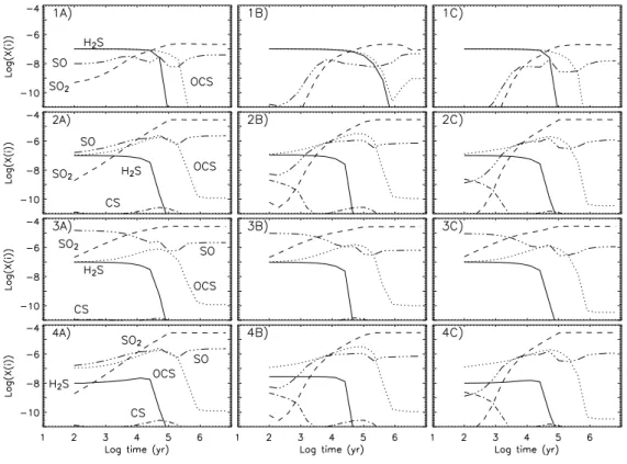
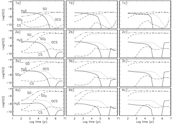
2Fig. 2. Evolution of the SO2, SO, H2S, OCS and CS abundances with respect to H2 as
a function of time, for the three pre-evaporation gas phase compositions A (left panels), B (central panels), and C (right panels) and the four grain mantle compositions (1 to 4, from the top to the bottom). The gas temperature is 100 K and the H2 density is 107
cm−3.
We have run the four models listed in Table 2, each with the three different gas-phase compositions (A, B, and C) prior to evaporation, for gases with temperatures of 100 K and 300 K, and densities of 105
cm−3, 106
cm−3 and 107
cm−3. In this section, we give
some sense of the major features of the chemistry of the sulphur-bearing species. Fig. 2 shows the evolution of the abundances of the SO2, SO, H2S, OCS and CS
molecules, with respect to H2, for the four models and three gas-phase compositions
(with T=100 K and n(H2)=107 cm−3). There are clearly differences among the models,
at times earlier than 104
yr, due to the different initial compositions whereas after 104
yr the three gas phase compositions give similar results. For example, for Models 1, 2 and 4, the compositions B and C give lower SO and SO2 abundances than the composition
Fig. 3. Evolution of the SO2, SO, H2S, OCS and CS abundances with respect to H2
as a function of time, using pre-evaporated gas phase composition A and the four grain mantle mixtures (1 to 4, from the top to the bottom). The gas temperature is 100 K and the density is 105 cm−3 (a, left panels), 106 cm−3 (b, central panels) and 107 cm−3 (c,
right panels).
results for Model 3. For sake of simplicity, in the following, we will discuss composition A, but the results do not change qualitatively assuming the B or C compositions.
Figs. 3 and 4 show the evolution, at 100 K and 300 K respectively, of the abundances of the main S-bearing species for the four grain mantle compositions of Table 2 at the three different densities. In all the models depicted, SO and SO2are the most abundant species
at late times. The final large amounts of SO2 are more noticeable in Models 2-4, where
large amounts of gaseous sulphur are available. At a temperature of 100 K and a density between 106and 107cm−3, the SO
2molecule becomes more abundant than SO after 104
-105 yr, mainly because of the neutral–neutral reaction O + SO → SO
2+ photon. Note
that this radiative association reaction is critical because of the high abundance of atomic O in the pre-evaporative gas. At 300 K, the SO2molecule is formed less efficiently via this
mechanism since it possesses an inverse dependence on temperature (see Table 3, reaction 756) but it is still as abundant as SO after 2 × 10⁵
yr for a density of 105
cm−3, and after 103yr for a density of 107 cm−3(see Fig. 4). At 300 K, OH is quickly (≤ 102yr) formed
through the reaction H2 + O → OH + H so that SO2 can be formed by the reaction
Fig. 4.Same as Fig. 3 but with a temperature of 300 K.
pre-evaporated gas-phase is crucial to produce the high abundance of OH at early times, contrary to what was found in previous models (e. g. Charnley 1997). In Model 3, where the initial sulphur is mostly in S2, the SO molecule is very quickly (≤ 102 yr) formed, as
S2 directly leads to SO through the reaction S2 + O → SO + S.
Now, let us look at the chemistry of hydrogen sulphide, OCS, and CS. The initial H2S abundance (see Table 2), dips sharply after 104yr in all models but increases after
106
yr for models 2 to 4 at 300 K. The decrease of the H2S abundance at 104 yr is
produced by the attack on H2S by H3O+, more abundant than H +
3 in regions, such as
hot cores, where water has a large abundance. The reaction between H3O+and H2S yields
protonated hydrogen sulphide (H3S+), which dissociatively recombines with electrons to
form HS at least part of the time: H3S+ + e− →HS + H + H. The HS product is itself
depleted by the reaction HS + O → SO + H. At 300 K, H2S is efficiently formed at
later times (≥ 105 yr) by a series of reactions that starts with the destruction by cosmic
ray-induced photons of SO and SO+ to produce atomic sulphur. Atomic sulphur is then
hydrogenated into HS first, and then H2S (with intermediate steps in which the unusual
species HS+2, H3S +
2, HS2 and H2S +
2 are formed). Note that at lower temperatures S is
oxygenated rather than hydrogenated, whereas at 300 K atomic oxygen goes into water and, therefore, S can be hydrogenated eventually.
As in the case of H2S, the initial (adopted) abundance of OCS is that derived from
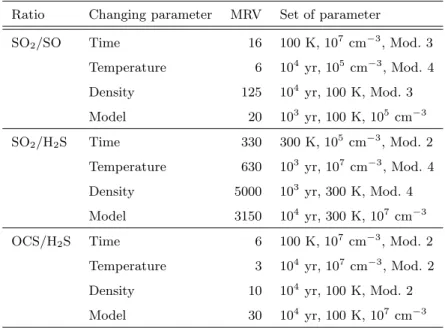
Table 6.Maximum sensitivity of the abundance ratios to assorted parameters.
Ratio Changing parameter MRV Set of parameter
SO2/SO Time 16 100 K, 107 cm−3, Mod. 3
Temperature 6 104 yr, 105 cm−3, Mod. 4
Density 125 104 yr, 100 K, Mod. 3 Model 20 103 yr, 100 K, 105 cm−3 SO2/H2S Time 330 300 K, 105 cm−3, Mod. 2
Temperature 630 103 yr, 107 cm−3, Mod. 4
Density 5000 103
yr, 300 K, Mod. 4
Model 3150 104
yr, 300 K, 107
cm−3
OCS/H2S Time 6 100 K, 107 cm−3, Mod. 2
Temperature 3 104
yr, 107
cm−3, Mod. 2
Density 10 104 yr, 100 K, Mod. 2
Model 30 104
yr, 100 K, 107
cm−3
gas phase, OCS is destroyed later than H2S. Under some conditions, e.g. T = 100 K and
n(H2) = 106–107cm−3, this molecule maintains a sizable if reduced abundance. Actually,
at T = 100 K and n(H2) = 106–107cm−3, there is even a temporary increase in the OCS
abundance from ∼ 10−7 to ∼ 10−6 (see Figure 3). The OCS molecule is mostly formed
by the radiative association reaction CO + S → OCS + PHOTON and this reaction is aided by the high density.
Unlike the other species, the CS molecule does not start on grain mantles in our cal-culations, but is part of the pre-evaporative gas. For composition A, its initial abundance is rather low. At 100 K, the initial CS is destroyed increasingly efficiently as density in-creases and its abundance never goes over 10−9. At 300 K, CS is efficiently produced at
high density after 103yr and it can be as abundant as 10−8. For compositions B and C,
there is significantly more CS present initially, especially for composition B, which con-tains 50 times more CS than in composition A. The initial CS is more slowly destroyed using compositions B and C than using composition A under the conditions depicted in Fig. 2 for Models 2 and 4.
3.2. Abundance ratios
Abundance ratios between sulphur-bearing species are exceedingly important because the use of fractional abundances (X(i) = N (i)/N (H2)) as chemical clocks introduces an
additional parameter in the analysis – the H2 column density (N(H2)) in the emitting
region – which is rarely well constrained observationally. Moreover, the abundance ratios are less sensitive to the initial amount of sulphur species compared with absolute abun-dances. For example, an initial abundance of S or S2 two times less than those used in
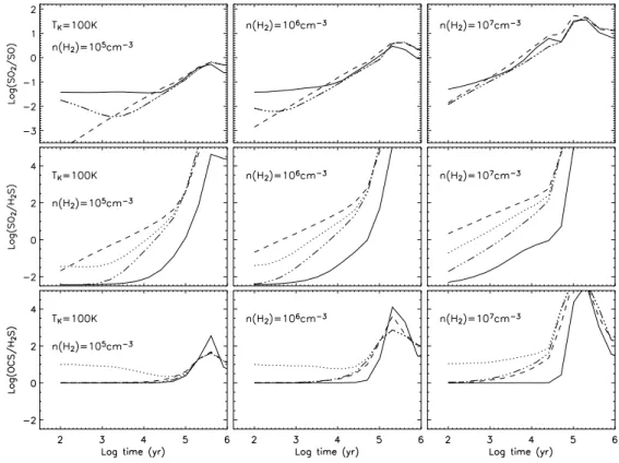
Fig. 5. Evolution of the abundance ratios SO2/SO (upper panels), SO2/H2S (middle
panels) and OCS/H2S (lower panels) as functions of time for composition A, a gas
tem-perature of 100 K, and densities of 105cm−3(left panels), 106cm−3 (central panels) and
107 cm−3 (right panels). The solid, dashed-dotted, dashed, and dotted lines represent
results from Models 1,2,3, and 4, respectively. In the upper panels, the results of Model 2 and and 4 are the same and represented by dashed-dotted lines.
abundance ratios are typically used to put contraints on chemical models, when the two species trace the same region.
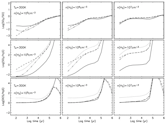
Figs. 5 and 6 show the evolution of the abundance ratios SO2/SO, SO2/H2S and
OCS/H2S, at 100 K and 300 K for three densities using composition A and all four models.
The overall sense of these figures is that the computed ratios are more sensitive to the gas temperature, the density, and the (poorly known) form of sulphur in grain mantles than to the time (particularly for t ≤ 3 × 10⁴yr) or to the gas phase chemical history of
the cloud. As a first step in quantifying the sensitivity of the studied abundance ratios to the different parameters, we report in Table 6 the maximum relative variation (MRV) for the three abundance ratios. These are obtained by changing the parameters time, temperature, density, model within the following considered ranges: time, 103
-104
yr; temperature, 100-300 K; density, 105
-107
cm−3; grain mantle composition, Models 1-4. The MRV is determined for each parameter by varying this parameter within the stated range while holding the others fixed at the set of values shown in Table 6. These sets lead to the strongest changes; hence the term ”maximum relative variation”. For example,
Fig. 6.Same as Fig. 5 but with a temperature of 300 K.
the maximum variation of the SO2/SO ratio produced by an increase of the time from
103 to 104 yr is 16 and it is obtained for a temperature of 100 K, a density of 107cm−3
and Model 3.
The SO2/H2S ratio shows the largest variations with time, but, unfortunately, also
with differing physical conditions and mantle mixtures. Indeed the ratio is more sensitive to the latter parameters than to the time, for t ≤ 3 × 10⁴
yr. The OCS/H2S ratio is less
sensitive to the different mantle mixtures and physical conditions, except at late times (≥ 105
yr). Unfortunately, however, this ratio is not sensitive to the time at t ≤ 105
yr either. The SO2/SO ratio shows significant variations with respect to the different mantle
compositions, and different densities and temperatures at relatively early times (≤ 104
yr). These variations mask completely the dependence on the time, which is, anyway, moderate at 100 K with the exception of the high density case, and small at 300 K.
To gain an understanding of the sensitivities of these abundance ratios in addition to that obtained from the MRV analysis, we follow the variations of SO2/SO, SO2/H2S
and OCS/H2S compared with reference ratios computed from Model 2 at 103 yr for a
temperature of 100 K and a density of 105
cm−3 (left panels of Fig. 5). The reference
SO2/SO ratio is ∼ 5×10⁻³and increases by only a factor of 2 by 104yr. However, a similar
increase can also be due to an underestimate of the density by a factor of 10 (note that if nH2 = 107 cm−3, the SO2/SO ratio increases by a factor of 20). Also, the reference
mixture. The reference SO2/H2S ratio is 0.01 and increases by one order of magnitude
at 104
yr. An increase in density (to 107
cm−3) or in temperature (to 300 K) gives
respectively a ratio of 0.3 or 0.1. The largest variation is seen if both the temperature and the density increase, so that the SO2/H2S ratio jumps to 160. A different mantle
mixture leads to ratios between 3 × 10⁻³ and 0.3 (at the reference time). The reference
OCS/H2S ratio is 1 and shows little to no sensitivity to time until 104yr, but also evinces
little change with temperature, density and mantle composition, with the exception of Model 4 which gives a ratio enhanced by a factor of ∼10 because the abundance of H2S
is 10 times less than in Models 1, 2, and 3.
4. Discussion
4.1. Comparison with previous models
The most recent papers focussing on the detailed modelling of sulphur chemistry in hot cores are those of Charnley (1997) and Hatchell et al. (1998). The adopted chemistry is roughly the same in the two models, but they differ in the value of the activation energy barrier for the destruction of H2S by atomic hydrogen (H2S + H → HS + H2). In
particular, Hatchell et al. used a value of 350 K while Charnley used a value of 850 K. Although there is some experimental support for a variety of choices, here we are using an energy barrier of 1350 K, based on the recent experiment by Peng et al. (1999) in the 300-600 K range. The difference in the activation energy barrier for the H2S + H
reaction causes significant variations in the models. While we obtain results similar to the Charnley model for 100 K, H2S destruction occurs at later times in our model for
T = 300 K. Moreover, the high value of the energy barrier has significant consequences on the SO and SO2abundances of our model with respect to the above two models. For
example at 104 yr, our model predicts SO and SO
2 abundances 6 and 30 times lower
than Charnley’s model, using the same parameters and initial conditions. Overall, and in addition to this, our results are different from these two models primarily because we are assuming different initial gas phase and/or mantle compositions. As already noted (in section 3.1), the large atomic oxygen abundance is, for example, an important difference in the pre-evaporated gas phase composition. Another difference is that both Charnley and Hatchell et al. assume that the bulk of sulphur in the ice mantle is in the H2S form.
Our model 1 adopts a similar mantle mixture, with solid-phase OCS as abundant as H2S,
whereas models 2, 3 and 4 assume that the bulk of the sulphur lies in the S or S2 forms.
These two classes of models give very different results, as widely discussed in section 3. Actually, a novelty of this work is the consideration that the sulphur can be in the atomic or molecular form when evaporated from the grain mantles. However, we should emphasize that atomic S is very quickly locked into SO and SO2 molecules, so that we
for a gas at 300 K and 107cm−3, the S abundance decreases from 3 × 10⁻⁵to 1.5 × 10⁻⁹
in 103
yr by reacting with O2 to form SO. This explains why van der Tak et al. (2003)
did not detect atomic sulphur2
in the hot core region of the massive protostars that they studied, where the gas temperature and density are similar to those quoted above. In a slightly colder gas (∼ 100 K), atomic S would survive longer, but it would be very difficult to detect. In fact the intensity of the SI fine structure line at 25.249 µm is 1 × 10⁻¹²erg
s−1 cm−2, for a gas at 100 K and 107 cm−3, a source size of 2”, an H
2 column density
of 1023 cm−2 , and all the sulphur in atomic form (as our models 2 and 4 adopt). The
signal would be attenuated by the foreground dust of the cold envelope, whose H2column
density is also around 1023 cm−2, by about a factor of ten (using the extinction curves
in Draine 2003) putting the signal at the limit of the ISO-SWS detection (a typical rms is few times 10−13 erg s−1cm−2). Future investigations in the ISO database will be done
in order to check the possible presence of atomique sulphur in hot cores.
Hatchell et al. (1998) found the cosmic ray rate to be an important parameter chang-ing the timescales of the destruction of H2S and the formation of SO and SO2. The
standard value usually assumed is 1.3 × 10⁻¹⁷s−1 but there are some indications that it
can vary depending on the region (see van der Tak & van Dishoeck 2000). To check the dependence on ionization rate whether or not it can pertain to objects as dense as hot cores, we have run the models for three different cosmic ray ionization rates: 1.3 × 10⁻¹⁷,
1.3 × 10⁻¹⁶ and 1.3 × 10⁻¹⁵ s−1. The results for the S-bearing abundance ratios do not
strongly depend on this parameter at a density of 105
cm−3. At higher densities,
how-ever, an increase in the cosmic ray ionization rate speeds up the photodestruction of OCS, H2S and SO2 via cosmic ray-induced photons. For a cosmic ray ionization rate of
1.3 × 10⁻¹⁵ s−1, a temperature of 100 K and a density of 107 cm−3, the abundances
of H2S and OCS start to decrease before 103 yr and the maximum abundance of SO2
is 4.5 × 10⁻⁸ instead of 2 × 10⁻⁷ with Model 1 and composition A. Hence, as Hatchell
et al. (1998), we found that the adopted value of the cosmic ray rate may be an impor-tant parameter at high density whereas it has weak consequences on the results at lower densities.
Recently, Nomura & Millar (2003) reported a study of the chemical composition across the envelope of the massive protostar G24.3+0.15. In this study, they derived the density and temperature profile and computed the chemical composition of the gas as a function of the radius and time. Evidently, the Nomura & Millar (2003) model is more complete than ours in dealing with the physical structure of the protostar, for
2
van der Tak et al. (2003) argued that the non detection of the 25 µm line corresponds to an upper limit to the atomic sulphur of ≤ 5 × 10⁻⁸, computed by considering line absorption.
Indeed, this is an upper limit on the S abundance in the absorbing gas, i.e. the foreground cold gas, rather than the hot gas. The upper limit on the emitting hot core gas is much higher, as explained in the text.
this is the focus of their model. On the other hand, given its complexity, the model does not explore the robustness of the achieved results as a function of the necessary assumptions of the model itself, which is, on the contrary, the focus of our study. In the same way, Doty et al. (2002) studied the chemical composition across the envelope of the massive protostar AFGL 2591. Finally, a further degree of complexity has been added to the problem by Rodgers & Charnley (2003), who considered the evolution of a protostar, including the evolution of the thermal and physical structure of the envelope plus the chemical evolution. As in the previous case, the advantage of having a better description of the protostar comes along with the disadvantage of a lack of exploration of the robustness of the results as a function of the chemical network utilized. In these three models, the authors assumed that sulphur was only evaporated from the grains mantles in the OCS and H2S forms for Nomura & Millar (2003) and only in the H2S form for Doty
et al. (2002) and Rodgers & Charnley (2003). We have discussed above the problem with the assumption that sulphur is totally frozen onto OCS and H2S, and showed that the
resulting S-bearing abundances depend dramatically on this assumption. The conclusion is the same if considering a model where sulphur is only in H2S (as discussed at the end
of Sect. 4.2). It comes as no surprise, therefore, that our results are different from those of these more detailed approaches.
4.2. Comparison with observations
In the following, we consider the case of two well studied hot cores: the massive Orion KL and the low mass IRAS16293-2422 hot cores. Orion KL is a complex region where several energetic phenomena are present. High resolution, interferometric observations have shown that different molecules originate in different components, especially for the OCS, SO and SO2 molecules (e.g. Wright et al. 1996). It is evidently a very crude
approximation to attribute all the S-molecule emission to the hot core, but lacking a better understanding of the region we will try to compare the observed abundances with our model predictions. First, in order to minimise the number of parameters, we will compare available observations with computed abundance ratios. The SO, SO2, H2S
and OCS column densities have been derived by Schilke et al. (2001) and Sutton et al. (1995) to be 2.3 × 10¹⁷, 6 × 10¹⁶, 1.2 × 1016 cm−2 and 9 × 1015 cm−2, respectively. All
these column densities are beam-averaged, with a beam of ∼ 10′′. For simplicity, we
will assume that the emission originates in the hot core region with T = 200 K and n(H2) = 107cm−3(Wright et al. 1992). The comparison of the abundance ratios derived
from the above column densities with our model predictions shows that none of the four models of Sect. 2.1 reproduces the observed data. However, the ratios can be reproduced by a model similar to Model 2, where the initial abundance of atomic sulphur injected into the gas phase is 3 × 10⁻⁶, i.e. ten times lower than the abundance used in Model 2.
Table 7. Observed and modelled abundances of SO, SO2, H2S, OCS and CS towards
the IRAS16293-2422 hot core.
Species observed Model 2 Model 2’ SO 1.7 × 10⁻⁶ 5 × 10⁻⁷ 4 × 10⁻⁷
SO2 5.4 × 10⁻⁷ 10−7 10−7
H2S 5.3 × 10⁻⁷ 10−7 10−7
OCS 1 × 10⁻⁶ 2 × 10⁻⁷ 10−7
CS - 1 × 10⁻¹¹ 2 × 10⁻¹²
We will call this model Model 2’. In that case, we obtain a good agreement between the model and the observations and derive an age of 4× 10³yr. Assuming the emission region
extends about 10” and an H2 column density of 8 × 1023 cm−2 (Sutton et al. 1995), the
observed abundances of SO, SO2, H2S and OCS are reproduced to within a factor of 10.
On the contrary, the CS abundance is underestimated by three orders of magnitude by our model, probably because CS emission does not originate in the hot core. Note that, given the complexity of the region, a better analysis would require an understanding of the H2 column density associated with the S-bearing molecules.
In the case of the low-mass protostar IRAS16293-2422, multifrequency observations of H2S, OCS, SO and SO2have been reported and analyzed by sophisticated models, which
take into account the density and temperature structure of the source, as well as the abundance profile of each studied molecule (Sch¨oier et al. 2002; Wakelam et al. 2004). Both Sch¨oier et al. (2002) and Wakelam et al. (2004) found the following abundance ratios in the inner warm region where the dust mantles evaporate (Ceccarelli et al. 2000a): SO2/SO=0.3, SO2/H2S=1 and OCS/H2S=1.9.
The modelling of the density and temperature profiles of IRAS16293-2422, by Ceccarelli et al. (2000a), suggests a density of 107 cm−3 and a temperature of 100 K
in the hot core region. Fig. 7 shows the comparison between the observed and predicted ratios (assuming composition A) for the four models: only Model 2 reproduces the obser-vations, suggesting an age of ∼ 2 × 10³yr for the protostar. To check the robustness of
this result, we also tried a variety of intermediate mantle mixtures, between Model 2 and Model 3, with the following characteristics: (1) one-half of the initial mantle sulphur in atomic form and one-half in the form of S2, (2) one-quarter in S and three-quarters in S2,
(3) three-quarters in S and one-quarter in S2. In all three intermediate cases, the resulting
curves are very similar to those found for Model 3. The presence of molecular sulphur clearly determines the form of the curves and is inconsistent with these observations. The observed ratios are, however, well reproduced by Model 2’ (used for the comparison with Orion) giving an age, ∼ 3 × 10³ yr, very similar to the age derived by Model 2.
Finally, both Model 2 and Model 2’ predict fractional abundances at the optimum times in good agreement (within a factor of 5-10) with those observed, as reported in Table 7.
SO2/SO SO2/H2S OCS/H2S Mod. 2 SO2/SO SO2/H2S OCS/H2S Mod. 1 SO2/SO SO2/H2S OCS/H 2S Mod. 3 SO2/SO SO2/H2S OCS/H2S Mod. 4
Fig. 7. Comparison between the observed ratios SO2/SO, SO2/H2S and OCS/H2S
to-wards IRAS16293-2422 and the theoretical predictions of four models (Mod. 1, 2, 3 and 4; all with composition A) for a gas temperature of 100 K and a density of 107
cm−3.
The grey empty boxes, if shown, represent those instances in which particular calculated ratios are in agreement for a range of times with the observed ones taking into account the uncertainties in the observations. The grey filled box for Model 2 shows the time interval where all calculated ratios are in agreement with the observed ones.
Note that the CS abundance towards IRAS16293-2422 has not been derived (Sch¨oier et al. 2002; Wakelam et al. 2004) and that the abundances of the main S-bearing species predicted by Model 2 and 2’ are very similar until 104yr. This comparison suggests that
the majority of the sulphur is released into the gas phase in its atomic form or quickly (t ≤103yrs) converted to it, and that the abundance of the H
2S molecule injected in the
gas phase from the grains mantles cannot be much less than 10−7.
The age determined for IRAS16293-2422 is relatively short compared with the pre-vious estimates (∼ 104 yr) (Ceccarelli et al. 2000b; Maret et al. 2002; Wakelam et al.
2004). However, our newly determined age represents only the time from the evaporation of the mantles; the dynamical time needed to reach the required luminosity to form the observed hot core is an additional ∼ 3 × 10⁴yr.
The discussion of the best chemical age for IRAS 16293-2422 is based on models with the standard value of the cosmic ray ionization rate (1.3 × 10⁻¹⁷s−1). If we use a rate 10
times higher as suggested by Doty et al. (2004), the observations towards IRAS16293-2422 are no longer in agreement with Model 2, but with Model 1, although the derived age is
very similar. Indeed, the enhanced cosmic ray ionization rate speeds up the destruction of H2S, increasing the ratio SO2/H2S more rapidly without affecting significantly the
other ones. Consequently, the SO2/H2S curves on Fig. 7 are shifted to the right of the
figures, worsening the agreement with Model 2 but improving it with Model 1. In that case, the derived age is 5 × 10³
yrs and the predicted absolute abundances are between 15 and 20 less than the observed ones, however. Thus, a high cosmic ray ionization rate is no longer compatible with our hypothesis that mantle evaporation leads quickly to high gas-phase abundances of atomic sulphur. The high cosmic ray ionization rate has also a consequence on the O2abundance pedicted to be ∼ 10−6at 103yr with Model 1 whereas
it is predicted to be two orders of magnitude lower with the standard value of the cosmic ray ionization rate and Model 2. However, at present one cannot choose between the two conditions (large abundances of S in the gas phase or large cosmic-ray ionization rate). High sensitivity observations of atomic sulphur (see Sect. 4.1) are needed to put stringent constraints on chemical models.
Another way to confirm our hypothesis of a large initial abundance of atomic sulfur would be a careful study involving several other protostars at different stages of evolution. The strongest prediction of our models 2 to 4 is the large (>∼ 10−5) amount of SO
2at late
times, compared with models that start with little sulphur evaporated from the grains. There is some evidence for SO2abundances in high-mass hot cores as large as 10−6 (van
der Tak et al. 2003), suggesting that an initial amount of sulphur at least higher than 10−6 is needed. But our prediction of large SO2 abundances in more evolved hot cores
with ages larger than ∼ 105 yr, does not pertain to the Orion and IRAS16293-2422 hot
cores (as found in the present work).
Quantitative comparisons with observations of other hot cores reported in the liter-ature, such as the observations by Hatchell et al. (1998) and Buckle & Fuller (2003), are difficult to carry out since the abundances determined by these authors are averages along the line of sight and beam-averaged. Hence, their analyses do not take into account the physical structure of the source. Finally, van der Tak et al. (2003) report the study of the S-bearing molecular abundance in half a dozen massive protostars. In this case, an attempt to disentangle the outer envelope and inner core has been done, but the anal-ysis is not accurate enough to derive abundance ratios to compare with detailed model predictions; rather, the authors just give order-of-magnitude jumps of abundance in the inner hot core regions. van der Tak et al. (2003) compared the measured abundances with the model predictions by Doty et al. (2002), and argued that OCS is the main sulphur bearing molecules on the mantles, because its predicted abundance is otherwise too low. We ran a model where sulphur is in solid OCS, to test this suggestion, and we found that it leads to results very similar to those of Model 1 (where sulphur is evaporated from the grain mantles in the H2S and OCS forms), because OCS has almost the same chemical
behavior as H2S. Although OCS is destroyed at later times, the differences in the SO
and SO2 formation are not significant and the same discussion about Model 1 is valid.
5. Conclusions
We have studied in detail the influence of the mantle form of sulphur on the post-evaporative gas-phase abundances of S-bearing molecules in hot star-forming regions, with the goal of understanding whether those molecules can be used to estimate ages. We considered four different reasonable mantle mixtures, from which gas-phase H2S,
OCS, S and S2 emerge after a process of evaporation and, for the last two species,
possible rapid reaction, with different relative abundances, joining other species in the gas-phase prior to evaporation. We then followed the post-evaporative chemical evolution, with an emphasis on the abundance ratios of the main sulphur-bearing species for realistic physical conditions present in hot cores. Our results show that none of the ratios involving the four most abundant S-bearing molecules, namely H2S, OCS, SO and SO2, can be
easily used by itself for estimating the age, because the ratios depend at least as strongly on the physical conditions and on the adopted grain mantle composition as on the time. Also, the abundance of atomic oxygen in the gas phase, if not correctly accounted for, can seriously affect the chemistry. The situation, however, is not totally hopeless, because a careful comparison between observations and model predictions can give some useful hints on time estimates, and on the mantle composition. Such a careful analysis has to be done on each single source, however, for both the physical conditions and mantle composition can vary from source to source, so that the abundance ratios are not directly comparable. In practice, a careful derivation of the molecular abundances (which takes into account the source structure) coupled with a careful modeling of the chemistry at the right gas temperature and density is necessary.
We applied our model to two well studied hot cores: Orion KL and IRAS16293. For the S-bearing abundances towards Orion KL, we assumed that their emission arises from the hot core region (which is strongly debatable) and is not beam-diluted. We were not able to reproduce all of the observed abundances ratios with any of our models. The agreement with Model 2 is satisfactory if we decrease the initial amout of atomic sulphur by a factor of 10. In that case, we derive a best age of 4 × 10³yr. However, the predicted
abundance of CS is three orders of magnitude lower than the observed one. Contrary to the case of Orion KL, the sulphur-bearing abundances though the low mass hot core of IRAS16293-2422 have been carefully determined through a sophisticated model (Sch¨oier et al. 2002), which takes into account the density and temperature structure of the source, as well as the abundance profile of each studied molecule. Using the standard value of cosmic ray rate, we found that Model 2, in which a large amount of atomic sulphur is initially present in the post-evaporative gas, best reproduces the observed abundance
ratios. In that case, we derived an age of ∼ 2 × 10³ yr from the evaporation era to the
current stage of this particular low mass hot core. If we decrease the initial amount of atomic sulphur in Model 2 as for Orion KL, the agreement is still good and gives a similar age. This analysis favors the hypothesis that sulphur is mainly evaporated from the grains in the atomic form or in a form quickly converted into it. On the contrary, if a higher rate is used as suggested by the recent modelling of Doty et al. (2004), best agreement occurs with Model 1, where no atomic sulphur can be found in the grain mantle and only H2S and OCS are initially present. The strongest prediction of our atomic sulfur-rich
model is the presence of large abundances of SO2, derived from this form of sulfur, at
late stages of hot cores. A futher systematic study of S-bearing-species towards older hot cores where the physical structure is well known would provide information to test this model. Moreover, the fact that not all of the sulfur need be initially in atomic form, given the reasonable agreement obtained using Model 2’, suggests that a signficant portion of the granular elemental sulphur may be tied up in materials such as iron sulphide (Keller et al. 2002).
Acknowledgements. V. W. wishes to thank Franck Selsis for helpful discussions on chemical modelling and uncertainties. V. W., C. C. and A. C. acknowledge support from PCMI. P.C. ac-knowledges support from the MIUR grant ”Dust and molecules in astrophysical environments”, and the ASI grant (contract I/R/044/02). E. H. acknowledges the support of the National Science Foundation (U. S.) for his research program in astrochemistry. The authors are grateful to Brunella Nisini and Malcolm Walmsley for useful discussions.
References
Aikawa, Y., Herbst, E., & Dzegilenko, F. N. 1999, ApJ, 527, 262 Baluteau, J.-P., Cox, P., Cernicharo, J., et al. 1997, A&A, 322, L33
Bergin, E. A., Kaufman, M. J., Melnick, G. J., Snell, R. L., & Howe, J. E. 2003, ApJ, 582, 830
Boogert, A. C. A., Helmich, F. P., van Dishoeck, E. F., et al. 1998, A&A, 336, 352 Boogert, A. C. A., Tielens, A. G. G. M., Ceccarelli, C., et al. 2000, A&A, 360, 683 Brown, P. D., Charnley, S. B., & Millar, T. J. 1988, MNRAS, 231, 409
Buckle, J. V. & Fuller, G. A. 2003, A&A, 399, 567
Cardelli, J. A., Meyer, D. M., Jura, M., & Savage, B. D. 1996, ApJ, 467, 334 Caselli, P., Hasegawa, T. I., & Herbst, E. 1993, ApJ, 408, 548
Caselli, P., Hasegawa, T. I., & Herbst, E. 1994, ApJ, 421, 206 Caux, E., Ceccarelli, C., Castets, A., et al. 1999, A&A, 347, L1 Ceccarelli, C., Castets, A., Caux, E., et al. 2000a, A&A, 355, 1129
Ceccarelli, C., Hollenbach, D. J., & Tielens, A. G. G. M. 1996, ApJ, 471, 400
Ceccarelli, C., Loinard, L., Castets, A., Tielens, A. G. G. M., & Caux, E. 2000b, A&A, 357, L9
Charnley, S. B. 1997, ApJ, 481, 396
Charnley, S. B., Rodgers, S. D., & Ehrenfreund, P. 2001, A&A, 378, 1024 Charnley, S. B., Tielens, A. G. G. M., & Millar, T. J. 1992, ApJ Lett., 399, L71 Chiar, J. E., Adamson, A. J., & Whittet, D. C. B. 1996, ApJ, 472, 665
Dickens, J. E., Irvine, W. M., Snell, R. L., et al. 2000, ApJ, 542, 870 Doty, S. D., Sch¨oier, F. L., & van Dishoeck, E. F. 2004, A&A, in press
Doty, S. D., van Dishoeck, E. F., van der Tak, F. F. S., & Boonman, A. M. S. 2002, A&A, 389, 446
Draine, B. T. 2003, ARA&A, 41, 241
Gerakines, P. A., Whittet, D. C. B., Ehrenfreund, P., et al. 1999, ApJ, 522, 357 Gibb, E. L., Whittet, D. C. B., Schutte, W. A., et al. 2000, ApJ, 536, 347 Hartquist, T. W., Dalgarno, A., & Oppenheimer, M. 1980, ApJ, 236, 182 Hasegawa, T. I. & Herbst, E. 1993, MNRAS, 261, 83
Hasegawa, T. I., Herbst, E., & Leung, C. M. 1992, ApJS, 82, 167
Hatchell, J., Thompson, M. A., Millar, T. J., & MacDonald, G. H. 1998, A&A, 338, 713 Hollenbach, D. & McKee, C. F. 1979, ApJS, 41, 555
Keane, J. V., Tielens, A. G. G. M., Boogert, A. C. A., Schutte, W. A., & Whittet, D. C. B. 2001, A&A, 376, 254
Keller, L. P., Hony, S., Bradley, J. P., et al. 2002, Nat, 417, 148 Lee, H.-H., Bettens, R. P. A., & Herbst, E. 1996, A&AS, 119, 111 Lis, D. C., Keene, J., Phillips, T. G., et al. 2001, ApJ, 561, 823
Maret, S., Ceccarelli, C., Caux, E., Tielens, A. G. G. M., & Castets, A. 2002, A&A, 395, 573
Meyer, D. M., Jura, M., & Cardelli, J. A. 1998, ApJ, 493, 222
Millar, T. J., Farquhar, P. R. A., & Willacy, K. 1997a, A&AS, 121, 139 Millar, T. J., MacDonald, G. H., & Gibb, A. G. 1997b, A&A, 325, 1163 Nomura, H. & Millar, T. J. 2003, A&A, in press
Pagani, L., Olofsson, A. O. H., Bergman, P., et al. 2003, A&A, 402, L77 Palumbo, M. E., Geballe, T. R., & Tielens, A. G. G. M. 1997, ApJ, 479, 839 Peng, J., Hu, X., & Marshall, P. 1999, J. Phys. Chem., 103, 5307
Pineau Des Forˆets, G., Roueff, E., Schilke, P., & Flower, D. R. 1993, MNRAS, 262, 915 Rodgers, S. D. & Charnley, S. B. 2003, ApJ, 585, 355
Ruffle, D. P., Hartquist, T. W., Caselli, P., & Williams, D. A. 1999, MNRAS, 306, 691 Ruffle, D. P., Rae, J. G. L., Pilling, M. J., Hartquist, T. W., & Herbst, E. 2002, A&A,
381, L13
Scappini, F., Cecchi-Pestellini, C., Smith, H., Klemperer, W., & Dalgarno, A. 2003, MNRAS, 341, 657
Schilke, P., Benford, D. J., Hunter, T. R., Lis, D. C., & Phillips, T. G. 2001, ApJS, 132, 281
Sch¨oier, F. L., Jorgensen, J. K., van Dishoeck, E. F., & Blake, G. A. 2002, A&A, 390, 1001
Schutte, W. A., Tielens, A. G. G. M., Whittet, D. C. B., et al. 1996, A&A, 315, L333 Sofia, U. J., Cardelli, J. A., & Savage, B. D. 1994, ApJ, 430, 650
Sutton, E. C., Peng, R., Danchi, W. C., et al. 1995, ApJS, 97, 455
Tieftrunk, A., Pineau Des Forets, G., Schilke, P., & Walmsley, C. M. 1994, A&A, 289, 579
van der Tak, F. F. S., Boonman, A. M. S., Braakman, R., & van Dishoeck, E. F. 2003, A&A, 412, 133
van der Tak, F. F. S. & van Dishoeck, E. F. 2000, A&A, 358, L79 van Dishoeck, E. F. & Blake, G. A. 1998, ARA&A, 36, 317
Vastel, C., Polehampton, E. T., Baluteau, J.-P., et al. 2002, ApJ, 581, 315 Viti, S. & Williams, D. A. 1999, MNRAS, 305, 755
Wakelam, V., Castets, A., Ceccarelli, C., et al. 2004, A&A, 413, 609
Wright, M., Sandell, G., Wilner, D. J., & Plambeck, R. L. 1992, ApJ, 393, 225 Wright, M. C. H., Plambeck, R. L., & Wilner, D. J. 1996, ApJ, 469, 216