HAL Id: hal-00298308
https://hal.archives-ouvertes.fr/hal-00298308
Submitted on 30 Jan 2007
HAL is a multi-disciplinary open access
archive for the deposit and dissemination of
sci-entific research documents, whether they are
pub-lished or not. The documents may come from
teaching and research institutions in France or
abroad, or from public or private research centers.
L’archive ouverte pluridisciplinaire HAL, est
destinée au dépôt et à la diffusion de documents
scientifiques de niveau recherche, publiés ou non,
émanant des établissements d’enseignement et de
recherche français ou étrangers, des laboratoires
publics ou privés.
initial boundary conditions sensitivity and case study
evaluation
S. Gaber?ek, R. Sorgente, S. Natale, A. Ribotti, A. Olita, M. Astraldi, M.
Borghini
To cite this version:
S. Gaber?ek, R. Sorgente, S. Natale, A. Ribotti, A. Olita, et al.. The Sicily Channel Regional Model
forecasting system: initial boundary conditions sensitivity and case study evaluation. Ocean Science,
European Geosciences Union, 2007, 3 (1), pp.31-41. �hal-00298308�
www.ocean-sci.net/3/31/2007/
© Author(s) 2007. This work is licensed under a Creative Commons License.
Ocean Science
The Sicily Channel Regional Model forecasting system: initial
boundary conditions sensitivity and case study evaluation
S. Gaberˇsek1,2, R. Sorgente3, S. Natale1, A. Ribotti3, A. Olita1, M. Astraldi4, and M. Borghini4
1IMC – International Marine Centre Loc. Sa Mardini, 09170 Oristano, Italy
2University of Ljubljana, Department of Mathematics and Physics, Jadranska 19, Ljubljana, 1000-SI, Slovenia
3IAMC/CNR-Istituto Ambiente Marino Costiero, Sede di Oristano, c/o IMC-Centro Marino Internazionale Loc. Sa Mardini,
09170 Oristano, Italy
4ISMAR CNR sez. di La Spezia Forte Santa Teresa Pozzuolo di Lerici, 19036 La Spezia, Italy
Received: 30 March 2006 – Published in Ocean Sci. Discuss.: 17 May 2006 Revised: 1 August 2006 – Accepted: 17 August 2006 – Published: 30 January 2007
Abstract. The Sicily Channel Regional Model forecasting
system was tested using an optimization package for the initial and lateral boundary conditions. Spurious high fre-quency oscillations during the spin-up time were success-fully reduced both in duration and magnitude by optimizing the time tendency of the free surface elevation using the Vari-ational Initialization and Forcing Platform method developed in the framework of the Mediterranean Forecasting System Towards the Environmental Prediction project. The effect of optimization was most profound for the free surface eleva-tion, where all oscillations with periods shorter than 4 h were suppressed.
The overall forecast skill was assessed on a 5 day case study starting on 6 April 2005, characterized by a fast pas-sage of a deepening atmospheric low–pressure field with strong winds and marked wind direction change. We com-pared the predicted variables with in–situ and remotely sensed data. The forecasts of temperature, including the sea surface temperature, and salinity were quite successful, while the forecasted currents, especially within the surface layer, were not in good agreement with the measurements.
1 Introduction
The numerical simulation of the sea circulation over ex-tended coastal shelf areas, such as the central Mediterranean basin, is extremely important in order to asses the short and long term environmental variability. However, in a short range forecast (order of days) of ocean properties, the spin– up time becomes a problem of great importance especially at the coastal time scales where spurious oscillations and prop-agating waves are present in results for several days after the initialization. (Auclair et al., 2001).
Correspondence to: S. Gaberˇsek
Regional models instead of OGCM are used in order to capture the mesoscale scale phenomena. The use of Lim-ited Area Model (LAM) as SCRM at regional scale em-bedded into a coarse resolution ocean model (OGCM) rep-resents an efficient way to downscale the model solutions from the basin-scale (12.5 Km) to the regional scale (3 Km) through a one-way, off-line nesting at the open lateral bound-aries. This method was found to be computationally efficient and sufficiently robust to transmit information across the lat-eral boundaries without excessive distorsion (Sorgente et al., 2003).
The spin–up is the time needed by an ocean model to reach a state of physical equilibrium under the applied forcing. The results can not be trusted until this equilibrium is reached due to spurious noise in the numerical solution. For an ocean basin-scale circulation model the spin–up can take hundreds of years to achieve an equilibrium, while regional models, that do not include deep ocean basins, may be much quicker. In order to start a model run for operational forecast or re-search purposes, some variables need to be specified at initial time. These variables include potential temperature, salinity, free surface displacement and velocity fields.
One way to initialize models is by using climatological values of temperature and salinity from databases and as-suming the velocity field equal to zero at the start time (Fox-Rabinovitz et al., 2002). The model will adjust the velocity field in balance with the density and the forcing field. As the forcing is applied, the velocity field will respond to the initial condition with a transient flow that may be unrealistic. For this reason, the results from the beginning of ocean circula-tion model runs are usually not used. This kind of approach, commonly used to initialize global or basin scale models, is named “cold start”.
Another common way is to initialize an ocean model by using fields from a previous run of the same model. If the saved fields from a recent forecast of the same model are used to initialize a new simulation, we call this approach a
“warm start”. The main advantage is that the ocean state has already been adjusted to the initial condition and is available for use in prediction.
One can also use dynamically balanced forecast fields from a model with coarser spatial resolution to initialize a model with higher resolution, but the phenomena of the smaller scale are not captured in the initial conditions. This is again a “cold start” and this approach has been used in the Sicily Channel Regional Model (hereafter SCRM) forecast-ing system, that will be discussed later.
In the “cold start” used in the SCRM we applied an inno-vative tool based on the Variational Initialization and Forcing Platform (hereafter VIFOP) method (Auclair et al., 2000) in order to initialize and force the regional forecast system from the coarse grid solution. The aim is to reduce the ampli-tude of the spurious external gravity wave generated during the spin–up time and to assess the sensitivity of the SCRM forecasting system to optimized initial and lateral boundary conditions. Furthermore, we want to perform a quantitative evaluation of forecasted fields in a case study.
The SCRM has been implemented in the framework of the Mediterranean Forecasting System Towards the Environ-mental Prediction project (hereafter MFSTEP). The SCRM has been realized for the Central Mediterranean sub-basin including the Sicily and Sardinia Channels (hereafter SiC and SaC, respectively) and the wide Tunisian/Libyan shelf. Although there exist modeling studies of the area (Molcard et al., 2002; Pierini and Rubino, 2001), the SCRM is the first operationally used model.
This study area is characterized by a complex bathymetry with wide continental shelves, deep and shallow channels and wide abyssal plains. Its central position in the Mediter-ranean basin plays a crucial role in a passage of the super-ficial and intermediate water masses in transit between the Eastern and the Western Mediterranean sub-basins (hereafter EM and WM, respectively). It also prevents the water masses from the deep and bottom layers of the two basins from mix-ing. The hydrology in the study area can be described as a multi-layer system composed of a series of adjacent water masses both in the horizontal and in the vertical direction. The upper layer is occupied by a surface layer (0–100 m) of relatively fresh water of Atlantic origin, frequently called Modified Atlantic Water (hereafter MAW). It is described as a broad homogeneous layer that undergoes progressive mod-ifications becoming warmer and saltier as it spreads eastward toward the EM basin (Manzella, 1994; Moretti et al., 1993). The inflow of MAW from the SaC drives the so-called Al-gerian Current (hereafter AC) ant its pathway is influenced by the topography, the surface forcing and by the density gradient between the Atlantic and the Mediterranean waters. The lateral variations in density with the surrounding water masses render the AC unstable, with the generation of in-stabilities represented by rather energetic mesoscale eddies. The surface circulation is characterized also by meanders, semi-permanent cyclonic and anticyclonic gyres and eddies,
some of them associated with the instabilities of the AC and the meandering of the Atlantic Ionian Stream (hereafter AIS) (Lermusiaux, 1999; Lermusiaux and Robinson, 2001; Robin-son et al., 1999). The AIS is a summer feature and is the main transporter of the MAW from the SaC to the open Io-nian Sea, together with the Atlantic Tunisian Current flowing along the Tunisian-Libyan shelf break (Beranger et al., 2004; Sorgente et al., 2003). At the bottom part of the MAW there is a thin layer traced by means of a relative temperature min-imum located between depths of about 100 and 200 m. It has been associated to the Winter Intermediate Water, previ-ously formed in the WM by surface cooling of MAW during the winter (Fuda et al., 2000; Ribotti et al., 2004; Sammari et al., 1999). Between about 200 m and the bottom there are the Levantine Intermediate Water (hereafter LIW) and, below, the transitional Eastern Mediterranean Deep Water forming the Eastern Mediterranean Overflow Water (here-after EOW). The LIW is characterised by a relatively high salinity and temperature. From the EM the EOW flows west-ward at an intermediate depth of approximately 300 m to-wards the shallowest depths of the SiC through the Maltese Sill (Fig. 1), where it passes two sills at 360 and 430 m deep before spreading into the Tyrrhenian Sea. Here its stream bifurcates under topographic constraints and the Coriolis ef-fect, and partially mixes with the upper and lower local wa-ters (Sparnocchia et al., 1999; Astraldi et al., 2002).
The paper is structured as follows: in Sect. 2, the model setup is described; sensitivity tests using VIFOP are in Sect. 3; a case study is in Sect. 4; conclusions follow in Sect. 5.
2 Model setup
The numerical model used to simulate the ocean circula-tion at a regional scale over the Central Mediterranean re-gion is the Sicily Channel Rere-gional Model (SCRM) devel-oped within the MFSTEP project framework. It is based on the Princeton Ocean Model (POM) (Blumberg and Mellor, 1987), a three-dimensional, hydrostatic, free surface ocean model using the Boussinesq approximation. The horizontal mesh is orthogonal and the vertical coordinate is terrain
fol-lowing (σ ). The domain extends from 9◦to 17◦E and from
31◦to 39.5◦N, with horizontal resolution 1x, 1y of 1/32◦
(∼3.5 km) (Fig. 1). There are nx=257×ny=273 mesh points with 24 σ levels. The numerical model uses time splitting with the external (barotropic) and internal (baroclinic) mode time steps of 4 and 120 s, respectively. The bathymetry is based on a regular grid with spacing of 1 min, bilinearly in-terpolated onto a regular SCRM grid (3 km).
SCRM is driven through initial and lateral boundary con-ditions by a coarse resolution model using a one-way nest-ing of daily mean fields of temperature, salinity and veloc-ity from a weekly forecast (MFS1671, Madec et al., 1998). Forcing at the surface is done using an air-sea coupling
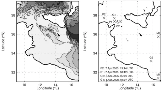
10 10 12 14 16 12 14 16 32 32 34 34 36 36 38 38 G1 G2 P1 P2 M1 M2 C1 C2 G1: 8.Apr.2005, 01:07 UTC G2: 8.Apr.2005, 02:09 UTC P1: 7.Apr.2005, 08:12 UTC P2: 7.Apr.2005, 13:14 UTC Longitude ( E) Longitude ( E) L a ti tu d e ( ✁ N ) L a ti tu d e ( ✁ N )
Fig. 1. The SCRM domain with bathymetry in grey contours from light (shallow) to dark (deep), contour interval 500 m. The thick black
line represents the coast line. Locations of in–situ measurements with XBT profilers are indicated with P1 and P2, Med–Argo gliders with G1 and G2, and with chained current meters with C1 and C2. Two additional points (M1,M2) indicate the location of model output points used for frequency analysis.
algorithm based on bulk parameterizations for the compu-tations of the momentum, heat and fresh water fluxes at the air-sea interface. The atmospheric fields needed for the sur-face boundary conditions were obtained using Skiron (Kallos et al., 1997).
The SCRM operational forecast system performs a 5 day ocean forecast in slave mode, i.e. it is re-initialized for each operational weekly forecast from the coarse
resolu-tion model. The 5 day forecasts start at 00:00 UTC on
each Wednesday. In this paper we discuss only a five day period from 6 April 2005 (00:00 UTC) to 11 April 2005 (00:00 UTC), during which there was an atmospheric low– pressure system passage over the SCRM domain. The rapid deepening was accompanied with strong winds at the sur-face.
Additional four experiments were performed using differ-ent dates (one 5 day forecast in each month from Septem-ber to DecemSeptem-ber 2004) with similar conclusions (results not shown in the paper). The April case was chosen because we initially planned to test the sensitivity to different atmo-spheric forcings as well.
3 VIFOP experiments
This section provides a description of sensitivity tests per-formed with VIFOP. VIFOP is a variational balanced initial-ization technique able to analyze the observations or the out-puts of regional scale or basin scale circulation models used as initial field or open boundary forcing of high resolution ocean models. Such method drastically reduces the ampli-tude of numerical transient processes following the
initial-ization by reducing the misfit of the initial field. The method is based on the minimization of a cost function involving data constraints as well as a dynamical penalty involving the tan-gent linear model. The optimization focuses on the exter-nal mode, more specifically on the time tendency of the free surface elevation. The tendency can be decomposed into a physical and numerical part and the goal is to minimize the spurious numerical tendency. For a detailed description of the package see Auclair et al. (2000) and for a more general text on data assimilation see Daley (1991) or Kalnay (2003). The VIFOP sensitivity tests included seven experiments, in which various combinations of initial and lateral bound-ary conditions were tested. Besides the prescribed fields of temperature, salinity and velocity, there is also an additional requirement for the volume transport (VT) across boundaries of the fine resolution model to match that of the coarse res-olution model (Zavatarelli and Pinardi, 2003). The VIFOP sensitivity tests were performed for a 5 day forecast period. The atmospheric fields used to provide the surface boundary conditions were the same as in the operational forecasting (Skiron). The coarse scale fields are from the Ocean General Circulation Model (OGCM) OPA, suited for the MFSTEP
project (MFS1671 – 1/16◦horizontal resolution, 71 vertical
levels). The sensitivity tests are described in Table 1, specify-ing the means of obtainspecify-ing both the initial (IBC) and lateral (LBC) boundary condition, as well as the volume transport adjustment (VT).
During the full optimization, the initialization of the ex-ternal mode is controlled by values of various parameters (e.g. weak or strong constraint during the optimization of the surface elevation tendency, optimization of the global divergence, optimization of the depth averaged velocities,
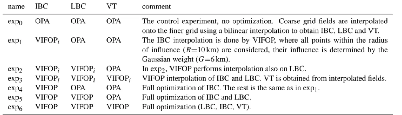
Table 1. List of sensitivity experiments. OPA and VIFOP stand for non–optimized and optimized IBC, LBC and VT, respectively. Subscript istands for interpolation only (no optimization).
name IBC LBC VT comment
exp0 OPA OPA OPA The control experiment, no optimization. Coarse grid fields are interpolated
onto the finer grid using a bilinear interpolation to obtain IBC, LBC and VT. exp1 VIFOPi OPA OPA The IBC interpolation is done by VIFOP, where all points within the radius
of influence (R=10 km) are considered, their influence is determined by the Gaussian weight (G=6 km).
exp2 VIFOPi VIFOPi OPA In exp2, VIFOP performs interpolation also on LBC.
exp3 VIFOPi VIFOPi VIFOPi VIFOP interpolation of IBC and LBC. VT is obtained from interpolated fields.
exp4 VIFOP OPA OPA Full optimization of IBC. The rest is the same as in exp1.
exp5 VIFOP VIFOP OPA Full optimization of IBC and LBC.
exp6 VIFOP VIFOP VIFOP Full optimization (LBC, IBC, VT).
0 6 12 18 24 Time (hr) ✂✁ (S v ) ✂✁ (S v ) -0.5 -0.5 0 0 0.5 0.5
Fig. 2. The total volume transport 8v (Sv) through the SCRM
boundaries for exp0(top) and exp6(bottom).
etc.). Various combinations were tested (not shown) and the best results were obtained by optimizing the global diver-gence and using the strong constraint on the free surface ten-dency. Unless otherwise noted this setup is used throughout the paper.
Surface or volume averaged quantities, like barotropic or baroclinic kinetic energy, respectively, do not reveal any dif-ferences among the experiments (not shown). Volume trans-port through lateral boundaries of the domain is very sen-sitive to the LBC. The total volume transport through the SCRM boundaries during the first day of simulation is shown
in Fig. 2. The high frequency oscillations of fluxes are
present in all experiments with interpolation only, regardless of method used (exp0,..,exp3). In fact, the volume transport
was similar in all experiments and for clarity only exp0 is
shown (Fig. 2 top panel). When VIFOP is used for the full optimization, the high frequency fluctuations in the total
vol-ume transport are of much smaller magnitude to begin with and become almost nonexistent after 12 h of simulations. It
is important to note the use of VIFOP for IBC only (exp4,
not shown) to some extent decreases the spurious oscilla-tions, but the additional optimization of LBC leads to even smoother volume transport (Fig. 2 bottom panel).
A further insight into impact of VIFOP was provided by a set of additional runs in which the model was integrated for two days only, instead of the regular 5 day forecast, but an ar-ray of variables was saved at each time step. The chosen vari-ables were the free surface elevation (output every barotropic time step of 4 s), and u component of velocity (output every baroclinic time step of 120 s). There were two sets of ten ad-jacent points at a constant latitude, spaced at 1x, close to the
eastern boundary at i) φ=31.4◦N to observe the shallow
wa-ter response, and ii) φ=35.75◦N to observe a response over
the deepest section of the domain (see Fig. 1 for location of points M1 and M2). The reason to monitor the chosen variables at ten adjacent points was to observe a transition from the boundary to the interior. The values at the outer-most points (i=nx) were determined by the lateral boundary conditions from the OGCM, and therefore changed linearly between the two subsequent daily values imposed through the LBC. The remaining nine points exhibited similar fea-tures during the simulation, so only values at the innermost point (i=nx−10) are discussed.
Since the high frequency oscillation associated with the model initialization diminish in time, a Fourier analysis of the whole time series is not appropriate. An alternative would be to perform a windowed Fourier analysis, but because we were interested in time–frequency localization of the signal, we used a wavelet analysis. It is now widely used in geo-physics (see reviews in Torrence and Compo, 1998, Kumar and Foufoula-Georgiou, 1997, Massel, 2001). During the analysis, the mother wavelet is scaled and translated along
the original signal to perform a convolution. By scaling
0 6 12 18 24 30 36 42 48 Time (hr) Power P e ri o d (m in u te s ) -4 -2 0 2 4 10 60 120 180 240 300 400 500 600 900 0 0.1 0.2 ✂✁☎✄ ✝✆✞✄ ✂✟✠✄
Fig. 3. (a) Time series of a detrended and normalized free surface
elevation at i=248, j=153 (ϕ=35.75◦N, λ=16.7◦E). (b) Wavelet power spectrum of the same time series. The contour interval values for normalized variance are from light to dark in range [1, 2, , 10]. The thick black line indicated the 95% confidence level for a red noise background, the hashed region represents the cone of influ-ence. (c) The global power spectrum, with the 95% confidence level (dashed line). See text for a more detailed explanation.
series can be picked up, analogous to Fourier periods. By shifting the wavelet function along the data series and per-forming the transformation, the location of the signals in the original data are determined.
We chose the Morlet wavelet, a plane wave modulated by an exponential decay, with a nondimensional frequency
ω0=6. An additional beneficial characteristic of this
par-ticular wavelet is its approximate one-to-one ratio between the Fourier period and wavelet scale (Torrence and Compo, 1998). The set of scales to be resolved depended on the an-alyzed variable, ranging from O(1 min) for the free surface displacement, to O(1 day) for the u component of velocity.
The data values from the model were first detrended and normalized by standard deviation, followed by the wavelet analysis. Each analysis presented in the paper (Figs. 3 and
4) consists of three panels. The top panel is detrended
and normalized model output data time series. The bottom panel is the local wavelet power spectrum in shaded con-tours with darker shades representing increasing values of normalized variance. A cone of influence indicates possi-ble errors related to the edge effects because the data series were finite, but the Fourier transform assumes the data to be cyclic (the transform is used for convolution purposes, see e.g. Torrence and Compo, 1998 for details). To the right is the global wavelet power spectrum, obtained by averaging in time. Lag-1 and lag-2 autocorrelation coefficients were calculated from the original time series in order to estimate the background red noise (increasing power with decreasing frequency/wavenumber) and determine the 95% confidence
0 6 12 18 24 30 36 42 48 Time (hr) Power P e ri o d (m in u te s ) -4 -2 0 2 4 10 60 120 180 240 300 400 500 600 900 0 0.1 0.2 ✂✁☎✄ ✝✆✞✄ ✂✟✠✄
Fig. 4. Same as Fig. 3 except for a simulation using VIFOP
opti-mized initial and boundary conditions.
level (Torrence and Compo, 1998). On the contour plot, the confidence level contours are shown with a thick black line while a thin dashed line is used on the global power spec-trum.
The wavelet analysis of the free surface elevation at the
northern point (M2, φ=35.75◦N) with no optimization shows
high frequency oscillations, with at least three distinct peri-ods, all statistically significant (Fig. 3bc). The shortest pe-riods are at around 20 and 40 min and they intermittently appear during the first 15 h of the simulation. The signal strength is barely above the red noise threshold. A stronger signal with a period of 120 min is present throughout the first 30 h of the simulations, visible as a thin, horizontal, dark re-gion on the contour plot and a distinct peak on the global spectrum. The cone of influence for longer periods sug-gests the influence of edge effects on the analysis. Indeed, the overall peak at approximately 850 min is an artifact of “cyclic” data, which vanishes if the length of the record is shortened to e.g. 24 h only. One way to avoid the spurious low frequency contamination would be to remove the low– order harmonics (48, 24 h) after detrending and normaliz-ing. Using optimized IBC and LBC, the wavelet analysis reveals an effective removal of all the significant high fre-quency signal (Fig. 4bc). Similar differences after applying optimization were observed also at the southern point (M1,
φ=31.4◦N).
Even though the timestep of the baroclinic mode was small enough to resolve the surface waves O(10 s), the correspond-ing wavelengths O(100 m) (Sverdrup et al., 1942) could not be resolved with the spatial resolution of the model, which was two orders of magnitude too big.
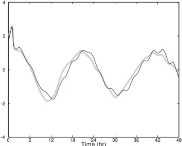
The most noticeable feature in the analysis of the u
component of the velocity at M2 (φ=35.75◦N) is the inertial
oscillation, with a period of around 22 h (Fig. 5). The wavelet analysis is not shown, since all the signal power is contained
0 6 12 18 24 30 36 42 48 Time (hr) -4 -2 0 2 4
Fig. 5. Time series of a detrended and normalized u component of
velocity optimized with VIFOP (thick gray line) and non-optimized (thin black line) at M2 (Fig. 1).
in the low–frequency oscillations in both optimized and non-optimized cases. The optimization of the initial and lateral boundary conditions using VIFOP does not affect the power spectrum. The only change is a reduction of small amplitude oscillations with an approximate period of 9 h towards the end of the 48 h period (wavelet power spectrum not shown). The inertial oscillation signal was also the most noticeable at
the second point further south (M1, φ=31.4◦N), although a
smaller depth of the point (50 m compared to 100 m) and its proximity to shallower sea bottom (∼130 m) influenced the dynamics.
The internal low-pass digital filter provided by VIFOP ef-fectively removes oscillations faster than ∼5 h. If they are attributed to noise the removal is welcome. If, on the other hand, the signal is true, one should be aware of the side ef-fects of using VIFOP. If the studied phenomena is on the time scale of 5 h or less, VIFOP at the current configuration should be used with caution.
4 Model evaluation
The results of numerical model were compared to mea-surements, including in–situ profiles of temperature, salin-ity and currents, and remotely sensed sea surface tempera-ture (SST). All the measured data was obtained directly from French Research Institute for Exploitation of the Sea, Ifre-mer (http://www.ifreIfre-mer.fr/mfstep/data management/wp14 data management) , except for the currents, which were ob-tained from two chains moored in the strict and deep pas-sages of the Sicily Strait.
The available in–situ measurements of temperature and salinity for the selected time period were quality controlled
0 100 200 300 400 500 600 700 Temperature ( C) Temperature ( C) Temperature ( C) Temperature ( C) D e p th (m ) 12 12 12 121314151617 1314151617 1314151617 1314151617 ✁ ✂ ✄☎ ✆ ✝✟✞ ✠✡ ☛ C ✁ ✂ ✄☎ ✆ ✝✟✞ ☞✌ ☛ C ✁ ✂ ✄☎ ✆ ✝✟✞ ✍ ☞ ☛ C ✁ ✂ ✄☎ ✆ ✝✟✞ ✎✏ ☛ C
point G1 point G2 point P1 point P2
Fig. 6. Measured in–situ temperature profiles (thick grey line)
ob-tained from Med-Argo gliders (G1, G2) and VOS-XBT (P1, P2), with interpolated model output (black squares) . The root mean square error (RMSE) is added for each plot. For spatial coordi-nates see Fig. 1.
and data points with incorrect quality flags were discarded. The original vertical coordinate of the measurements is pres-sure, which was transformed into depth using the hydro-static relation. If the salinity was available (points G1 and G2), a polynomial relation was used to calculate the water density as a function of temperature and salinity (Mellor, 1991), otherwise a constant reference density was assumed (ρ0=1025 kgm−3), for the hydrostatic calculation.
The temperature profile was generally well captured by the model at all points (Fig. 6). The exceptions were at sharp transitions where the model tends to smooth out the profile ( e.g. point G1 between 100 and 200 m). A discrepancy of
∼1◦C was found also at G2 where the model underpredicted
the depth of the mixed surface layer. The RMSE values are the lowest at points G2 and P2, because of the good agree-ment between the model and measureagree-ments at depths below 200 m.
The model derived salinity profile at G1 differs
substan-tially from the measurements (Fig. 7). While the model
predicts a ∼100 m thick top layer with constant salinity, the measured profile shows a large gradient in the surface layer, with almost constant salinity below 50 m. The depth of the eastward flowing less saline water in the top layer was overestimated by the model, but the origin of this er-ror can be traced to the lateral boundary conditions provided by OGCM. If the model profile is retrieved at another loca-tion in proximity to G1, the salinity in the top layer starts resembling the measured values. The predicted salinity pro-file at G2 matches the measurements quite well.
The second type of comparison was performed using re-motely sensed SST values. From the satellite data, 3-hourly
0 100 200 300 400 500 600 700 Salinity (psu) Salinity (psu) D e p th (m ) 37 3737.53838.539 37.53838.539 ✁ ✂✄ ☎ ✆✞✝ ✟ ✟ p s u ✁ ✂✄ ☎ ✆✞✝ ✆✠ p s u point G1 point G2
Fig. 7. Measured in–situ salinity profiles (thick grey line) obtained
from Med-Argo gliders (G1, G2) with interpolated model output (black squares) . For spatial coordinates see Fig. 1.
values (0.1◦ spatial resolution) of SST were obtained from
Ifremer ftp site (ftp.ifremer.fr/pub/ifremer/cersat/SAFOS1/ Products/ATLSST/2005). In order to retain high temporal resolution, the SST data used was not corrected for cloudi-ness, which is a regular procedure for 12 and 24-hourly prod-ucts. Thus, for days with a total cloud overcast, there were no data points available. Besides temperature, each data point contains also a quality control flag and only those with ex-cellent (5), good (4) or acceptable (3) values of confidence level were used. The third piece of information is the mean time at which the information was obtained (Brisson et al., 2001a). To proceed with the comparison, the model data was interpolated spatially onto the satellite grid and temporally to the time output determined by the time flag. An additional modification of the model postprocessing included extrapo-lation of the sea temperature profile to the depth of 1 cm (skin depth) by using the vertical temperature gradient between the top two model levels, which served as the SST for the com-parison with the satellite measurements.
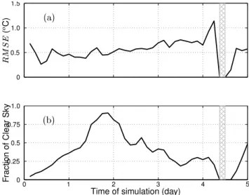
The temporal evolution of the root mean square error of SST shows a steady increase until it suddenly drops to zero, due to the total overcast with no visible pixels (Fig. 8a). The
average value of RMSE for the whole period was 0.54◦C.
The percentage of visible sky is shown on (Fig. 8b), with a steady decline after day 2 associated with the passage of an atmospheric low–pressure system.
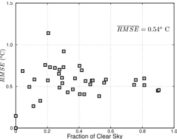
Another view of the impact of the number of pixels on the error is shown in Fig. 9. The RMSE has much smaller variability if there is approximately at least one third of the total number of pixels available. The overall value of RMSE does not change if only points above the one-third threshold are taken into account. It is interesting to note the reported
error of the satellite–derived SST is around 0.5◦C with the
cloudiness threshold of 0.6 (Brisson et al., 2001b), compara-ble to our findings.
0 0.25 0.5 0.75 1.0 0 0.5 1.0 1.5
Time of simulation (day)
✁ ✂ ✄☎ ( ✆ C ) F ra c ti o n o f C le a r S k y 0 1 2 3 4 5 ✝✟✞✡✠ ✝☞☛✌✠
Fig. 8. (a) Root Mean Square Error of SCRM predicted SST
evalu-ated with satellite-derived values. (b) Ratio of visible pixels (clear sky) to the total number of pixels over the water over the SCRM domain. Grey hatched area denotes the total cloud cover.
The model predicted SST has a small negative bias with
the mean error of –0.08◦C (not shown). To assess the
ef-fects of the optimization of IBC and LBC, the same compar-ison procedure for SST was repeated with the model output using VIFOP. The differences regarding the non–optimized IBC and LBC were negligible for the comparison with the measurements available for the case study.
Data from two chained sea–current meters was also used for model validation (see location of points C1 and C2 on Fig. 1). Both instruments are located in the Sicilian Channel and provide hourly observations of sea–current profiles with a vertical resolution of 8 (C1) and 4 m (C2). The strongest signal in the data were lunar semi-diurnal tidal oscillations
(M2) (Gill, 1982), which were removed by using a Doodson
X0 numerical filter (Schureman, 1958). The resulting data set had a strong high frequency noise with a period of 2 h, which was subsequently filtered out. The filtered measure-ments were then interpolated spatially and temporally onto the model levels and times, respectively.
The main reason for the chosen period of the case study was a passage of deepening atmospheric low–pressure field over the domain. The forecasted atmospheric fields (inter-polated to points C1 and C2) used for the surface bound-ary conditions indicate an increase in air temperature dur-ing the second and third day of the simulation, followed by a more rapid drop during the fourth day (thick gray line in Fig. 10a). The rising air temperature is accompanied by
strong southerly winds, peaking at approximately 18 ms−1
during the third day which were replaced by northwesterly winds (Fig. 10b) and temperature decrease. The evolution of the air temperature and wind resembles that of a classical warm/cold frontal passage. Due to insignificant differences
0 0.5 1.0 1.5
Fraction of Clear Sky
✁ ✂✄ ☎✆ ✝ ✞ 0 0.2 0.4 0.6 0.8 1.0 ✟✡✠ ☛✌☞ ✍ ✎✑✏✓✒✕✔✗✖✙✘
Fig. 9. Root Mean Square Error of the forecasted SST compared to
satellite derived values as a function of cloud coverage.
10 12 14 16 -200 -150 -100 -50 0 Time (days) T ( C ) D e p th (m ) 0 1 2 3 4 5 ✁✄✂✆☎ ✁✞✝✟☎ ✁✄✠✡☎
Fig. 10. Time series of (a) observed SST interpolated to point C2
(squares), forecasted by SCRM (black line), and air-temperature from the atmospheric model (thick grey line); (b) wind vector from the atmospheric model, interpolated to point C2. Upward point-ing arrow represents southerly winds; maximum wind speed was approximately 18 ms−1; (c) sea-current profile at C2, plotted every other level and every 3 h. Upward pointing arrow represents a north-ward current; maximum amplitude was approximately 1.2 ms−1.
in forecasted atmospheric parameters (wind and air temper-ature), and measured and forecasted SST between the two points (C1 and C2), data for only one point is discussed. The missing values of SST from the third to the fifth day are due to the predominantly overcast skies over the two points.
The oceanic response to the atmospheric forcing at C2 is visible comparing Figs. 10b and c. The observed sea currents at the topmost layer (depth of approximately 20 m) resem-ble the atmospheric forcing, albeit phase shifted by ∼18 h. Below 50 m, the response is much weaker and spread over
-100 -50 0 Time (days) D e p th (m ) 0 1 2 3 4 5
Fig. 11. Same as Fig. 10c, except for the point C1. Maximum
ve-locity was approximately 0.9 ms−1. Circles denote missing values.
-200 -150 -100 -50 0 Time (days) D e p th (m ) 0 1 2 3 4 5
Fig. 12. The forecasted currents at C1. Maximum velocity was
approximately 0.58 ms−1. The scaling of the current vectors is kept the same as in Figs. 10 and 11 for comparison.
a longer time scale. Even though there were no direct mea-surements of salinity and temperature at C2, the general char-acteristics were deduced from points P1 and G1 due to their spatial proximity (Fig. 1), but note that the data refers only to one sample per location and not the whole time series. In the top layer the water temperature rapidly decreases (Fig. 6), while the salinity increases (Fig. 7). Below 50 m, the water is colder and saltier, and it flows generally towards NW. The decoupled flow structure is consistent with the general struc-ture in the Sicily Channel, with the Atlantic Water (AW) at the surface and Levantine Intermediate Water (LIW) below (Manzella et al., 1988).
The differences in observed currents between C1 and C2 can be attributed to the local bathymetry. The Strait of Sicily, where both instruments are located, has a non–uniform bot-tom topography. From the coast of Tunisia (Cap Bon) to the southwestern tip of Sicily, there are two sills over which the currents are channeled (Manzella et al., 1990). Their po-sition roughly corresponds to C1 and C2 according to the bathymetry used for the SCRM. A possible branching of LIW could be evidenced by measurements from both points. Note that measured currents at C1 between depths of 50 and 100 m are consistently stronger and more uniform in direc-tion (Fig. 11), most likely due the channeling. The delay to the atmospheric forcing in the upper layer is similar to C2, but the direction-wise response is different, with cur-rents never obtaining strong southerly component, as in C2 (Figs. 10c and 11).
-200 -150 -100 -50 0 Time (days) D e p th (m ) 0 1 2 3 4 5
Fig. 13. Same as Fig. 12, except for the point C2. Maximum
veloc-ity was approximately 0.47 ms−1.
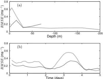
0 0 0.2 0.2 0.4 0.4 0.6 0.6 0.8 0.8 Depth (m) Time (days) ✁ ✂✄ (m s ☎ ✆ ) ✁ ✂✄ (m s ☎ ✆ ) 0 1 2 3 4 5 -200 -150 -100 -50 0 ✝✟✞✡✠ ✝☞☛✌✠
Fig. 14. Current velocity: (a) Time averaged RMSE as a function
of depth, and (b) depth averaged RMSE as a function of time for C1 (thin black line) and C2 (thick gray line).
The response of the surface layer in the model is not so straightforward to interpret. During the first day of simula-tion when the winds are northerly, the currents are accord-ingly southward in both points (Figs. 12 and 13). How-ever, when the strong forcing with southerly winds starts on the second day of simulation, lasting for approximately two days, the surface layer responds almost instantly, but with currents perpendicular to the wind. With the onset of northerly winds during the fourth day, the surface layer cur-rents in both points respond properly (Figs. 12 and 13). Note that the forecasted currents at the depth of 200 m at C1 are again stronger than at C2. Optimizing the boundary con-ditions did not significantly affect the simulated currents at either of the two points.
Another possible reason for the discrepancy are largely underestimated surface geostrophic currents. The simulated surface currents are perpendicular in direction and in phase with the atmospheric forcing, while the observed currents are consistent with the along-channel pressure gradient. It
appears that the model was not able to properly reproduce sub-surface horizontal pressure gradients.
For the statistical evaluation of the currents, two skill scores were calculated. The first one is a time averaged
RMSEat each level, the second one is a depth averaged
tem-poral evolution of RMSE. We constrained our analysis only on the magnitude of the currents, since the forecasted direc-tion is highly affected by the model resolved bathymetry.
High values of RMSE are found within the surface layer for both points (Fig. 14a). Note that the relatively lower values at C1 are caused by missing values in measurements (Fig. 11). The time series of depth averaged RMSE reveals maxima at both points during the period of strong surface currents forced by winds to which the model did not respond accordingly (Fig. 14b).
5 Conclusions
Unoptimized operational forecasts of SCRM contained spu-rious high frequency oscillations, lasting up to two days into the forecast. The oscillations mostly affected the barotropic variables, i.e. the free surface displacement and both com-ponents of barotropic velocity. The derived variables, such as the total volume transport, consisting of both baroclinic and barotropic modes, were consequently also affected by the noise. The amplitude was high enough to render the fore-cast useless. Baroclinic variables (components of velocity, temperature and salinity) did not contain the same type of noise.
In order to reduce the magnitude of the oscillations, an op-timization tool (VIFOP) was developed within the scope of MFSTEP. Because of the nature of the noise, we attempted to optimize only the time tendency of the free surface dis-placement. During the optimization, the spurious numerical time tendency was minimized without affecting the physical time tendency, which is the real signal. We tested various combinations of optimized boundary conditions (i.e. initial, lateral) and concluded that the best results were achieved by optimizing all of them. Spurious initial oscillations were suc-cessfully suppressed both in duration and magnitude by using VIFOP. The time needed for the full optimization of SCRM is on the order of 8 min per day of simulation, using a Linux PC with 2 GB of memory, of which approximately 1 GB was needed for VIFOP. Thus for the whole 5 day forecast which takes around 3 hours, the overhead of 40 min was not neg-ligible, but still acceptable compared to the total duration of the simulation.
We analyzed the effect of optimization by performing a wavelet analysis on one barotropic variable (free surface dis-placement) and one baroclinic variable (u component of ve-locity). The free surface oscillations with periods shorter than 4 h are effectively suppressed. The total volume trans-port which contained high amplitude oscillations during the first two days of forecast is vastly improved and useful for the
full 5 day duration of the simulation. The barotropic velocity field was dominated by inertial oscillations and the optimiza-tion process did not affect the main signal.
The forecast evaluation was performed by comparing the predicted variables with observations from in-situ and re-motely sensed measurements. Both temperature and salinity were predicted quite well, the only discrepancy occurred in the surface layer at one station and the source of error can be traced back to the prescribed IBC/LBC. The SST prediction also had a small error, but in order to resolve high temporal resolution we used the data not corrected for cloudiness. We concluded that the error of the SST prediction stays rather constant when the fraction of visible sky is above 0.35. The optimization procedure had no impact on prediction of SST, temperature, salinity and currents.
The verification of predicted currents resulted in lower confidence in forecasted values. This was especially the case within the surface layer, where the observed currents clearly responded to the atmospheric forcing (passing cold front with a rapid shift in wind direction), while the model did not man-age to create a similar response.
Ability of the SCRM to develop its own dynamics is in-hibited by OGCM forcing. A more detailed comparison of various operational settings, in which forecasts will be pre-ceded by hindcasts in order to develop high resolution fea-tures (both temporal and spatial) is left for the future.
Acknowledgements. This research has been realized in the
frame-work of EC MFSTEP project (EVK3-2001-00174) with an addi-tional support from the Marie Curie – ODASS fellowship (HPMD-CT-2001-00075 ODASS). The leading author is also grateful for the hospitality at the International Marine Center, and to his employer, University of Ljubljana, Department of Mathematics and Physics, for allowing the sabbatical leave. We are grateful to three anony-mous referees for their suggestions which helped to improve the paper.
Wavelet software was provided by C. Torrence and G. Compo, and is available at http://paos.colorado.edu/research/wavelets.
Edited by: N. Pinardi
References
Astraldi, M., Conversano, F., Civitarese, G., Gasparini, G., Rib-era d’Alcala, M., and Vetrano, A.: Water mass properties and chemical signatures in the central Mediterranean region, J. Mar. Syst., 155–177, 2002.
Auclair, F., Casitas, S., and Marsaleix, P.: Application of an In-verse Method to Coastal Modeling, J. Atmos. Ocean. Technol., 17, 1368–1391, 2000.
Auclair, F., Marsaleix, P., and Estournel, C.: The penetration of the Northern Current over the Gulf of Lions (Mediterranean) as a downscaling problem, Oceanol. Acta, 24, 529–544, 2001. Beranger, K., Mortier, L., Gasparini, G., Gervasio, L., Astraldi, M.,
and Crepon, M.: The dynamics of the Sicily Strait: a
compre-hensive study from observations and models, Deep-Sea Res. II, 411–440, 2004.
Blumberg, A. and Mellor, G.: A Description of a Three-Dimensional Coastal Ocean Circulation Model, in: Three Di-mensional Coastal Ocean Models, edited by Heaps, N., 1–16, American Geophysical Union, 1987.
Brisson, A., Le Borgne, P., and Marsouin, A.: Atlantic Sea Surface Temperature Product Manual, Tech. rep., Mto-France/DP/CMS, 22302 Lannion, France, 2001a.
Brisson, A., Le Borgne, P., and Marsouin, A.: Results of one year of preoperational production of GOES-8 derived SST., Cms report to eumetsat, Mto-France/CM, 22302 Lannion, France, 2001b. Daley, R.: Atmospheric Data Analysis, Cambridge Atmospheric
and Space Science Series, Cambridge University Press, 1991. Fox-Rabinovitz, M., Takacs, L., and Govindaraju, R.: A Variable
Resolution Stretched Grid General Circulation Model and Data Assimilation System with Multiple Areas of Interest: Studying Anomalous Regional Climate Events of 1998, J. Geophys. Res., 2002.
Fuda, J., Millot, C., Taupier-Letage, I., Send, U., and Bocognano, J.: XBT monitoring of a meridian section across the western Mediterranean Sea, Deep-Sea Res. I, 2191–2218, 2000. Gill, A. E.: Atmosphere-Ocean Dynamics, International
Geo-physics Series, Academic Press, 1982.
Kallos, G., Nickovic, S., Papadopoulos, A., Jovic, D., Kakaliagou, O., Misirlis, N., Boukas, L., Mimikou, N., G., S., J., P., Anad-ranistakis, E., and Manousakis, M.: The regional weather fore-casting system Skiron: An overview, in: Proceedings of the Sym-posium on Regional Weather Prediction on Parallel Computer Environments, 109–122, Athens, Greece, 1997.
Kalnay, E.: Atmospheric Modeling, Data Assimilation and Pre-dictability, Cambridge University Press, 2003.
Kumar, P. and Foufoula-Georgiou, E.: Wavelet analysis for geo-physical application, Rev. Geophys., 35, 385–412, 1997. Lermusiaux, P.: Estimation and study of mesoscale variability in
the strait of Sicily., Dynam. Atmos. Oceans, 255–303, 1999. Lermusiaux, P. and Robinson, A.: Features of dominant mesoscale
variability, circulation patterns and dynamics in the Strait of Sicily, Deep-Sea Res. I, 1953–1997, 2001.
Madec, G., Delecluse, P., Imbard, M., , and Levy, C.: OPA8.1 Ocean general Circulation Model reference manual, Note du Pole de modelisation,Institut Pierre-Simon Laplace (IPSL), France, 1998.
Manzella, G.: The seasonal variability of the water masses and transport through the Strait of Sicily, 33–45, AGU, 1994. Manzella, G., Gasparini, G., and Astraldi, M.: Water exchange
be-tween the eastern and western Meditarranean through the Strait of Sicily, Deep-Sea Res., 35, 1021–1035, 1988.
Manzella, G., Hopkins, T., Minnett, P., and Nacini, E.: Atlantic Water in the Strait of Sicily, J. Geophys. Res., 95, 1569–1575, 1990.
Massel, S. R.: Wavelet analysis for processing of ocean surface wave records, Ocean Engineer., 28, 957–987, 2001.
Mellor, G.: An equation of state for numerical models of oceans and estuaries, J. Atmos. Ocean. Technol., 8, 609–611, 1991. Molcard, A., Gervasio, L., Griffa, A., Gasparini, G.P., Mortier, L.,
and ¨Ozg¨okmen, T.: Numerical investigation of the Sicily Chan-nel dynamics: density currents and water mass advection, J. Mar. Syst., 36, 219–238, 2002.
Moretti, M., Sansone, E., Spezie, G., and De Maio, A.: Results of investigations in the Sicily Channel (1986–1990), Deep-Sea Res. II, 1181–1192, 1993.
Pierini, S. and Rubino, A.: Modeling the Oceanic Circulation in the Area of the Strait of Sicily: The Remotely Forced Dynamics, J. Phys. Oceanogr., 31, 1397–1412, 2001.
Ribotti, A., Puillat, I., Sorgente, R., and Natale, S.: Mesoscale cir-culation in the surface layer off the southern and western Sardinia island in 2000, Chem. Ecol., 20, 345–363, 2004.
Robinson, A., Sellschopp, J., Warn-Varnas, A., Leslie, W., Lozano, C., Haley Jr., P., Anderson, L., and P.F.J, L.: The Atlantic Ionian Stream, J. Mar. Syst., 129–156, 1999.
Sammari, C., Millot, C., Taupier-Letage, I., Stefani, A., and Brahim, M.: Hydrological characteristics in the Tunisia-Sardinia-Sicily area during spring 1995, Deep Sea Res. I, 46, 1671–1703, 1999.
Schureman, P.: Manual of Harmonic Analysis and Prediction of Tides, Tech. Rep. Special Publication No. 98, U.S. Department of Commerce, Coast and Geodetic Survey, 1958.
Sorgente, R., Drago, A. F., and Ribotti, A.: Seasonal variability in the Central Mediterranean Sea circulation, Ann. Geophys., 299– 322, 2003.
Sparnocchia, S., Gasparini, G., Astraldi, M., Borghini, M., and Pis-tek, P.: Dynamics and mixing of the Eastern Mediterranean out-flow in the Tyrrhenian basin, J. Mar. Syst., 301–317, 1999. Sverdrup, H., Johnson, M. W., and Fleming, R.: The Oceans, Their
Physics, Chemistry and General Biology, Prentice Hall, 1942. Torrence, C. and Compo, G. P.: A practical guide to wavelet
analy-sis, Bull. Am. Meteorol. Soc., 79, 61–78, 1998.
Zavatarelli, M. and Pinardi, N.: The Adriatic Sea modelling system: a nested approach, Ann. Geophysicae, 345–364, 2003.