The 1986?1989 ENSO cycle in a chemical climate model

HAL Id: hal-00303908

https://hal.archives-ouvertes.fr/hal-00303908

HAL is a multi-disciplinary open access

archive for the deposit and dissemination of sci-entific research documents, whether they are pub-lished or not. The documents may come from teaching and research institutions in France or abroad, or from public or private research centers.

L’archive ouverte pluridisciplinaire HAL, est destinée au dépôt et à la diffusion de documents scientifiques de niveau recherche, publiés ou non, émanant des établissements d’enseignement et de recherche français ou étrangers, des laboratoires publics ou privés.

The 1986?1989 ENSO cycle in a chemical climate model

S. Brönnimann, M. Schraner, B. Müller, A. Fischer, D. Brunner, E. Rozanov,

T. Egorova

To cite this version:

S. Brönnimann, M. Schraner, B. Müller, A. Fischer, D. Brunner, et al.. The 1986?1989 ENSO cycle in a chemical climate model. Atmospheric Chemistry and Physics Discussions, European Geosciences Union, 2006, 6 (3), pp.3965-3996. �hal-00303908�

ACPD

Full Screen / Esc

Printer-friendly Version

Interactive Discussion Atmos. Chem. Phys. Discuss., 6, 3965–3996, 2006

www.atmos-chem-phys-discuss.net/6/3965/2006/ © Author(s) 2006. This work is licensed

under a Creative Commons License.

Atmospheric Chemistry and Physics Discussions

The 1986–1989 ENSO cycle in a chemical

climate model

S. Br ¨onnimann1, M. Schraner1, B. M ¨uller1, A. Fischer1, D. Brunner1, E. Rozanov1,2, and T. Egorova2

1

Institute for Atmospheric and Climate Science, ETH Z ¨urich, Universit ¨atsstr. 16, 8092 Z ¨urich, Switzerland

2

PMOD/WRC, Dorfstr. 33, 7260 Davos, Switzerland

Received: 1 March 2006 – Accepted: 13 March 2006 – Published: 18 May 2006 Correspondence to: S. Br ¨onnimann ([email protected])

ACPD

Full Screen / Esc

Printer-friendly Version

Interactive Discussion

EGU

Abstract

A pronounced ENSO cycle occurred from 1986 to 1989, accompanied by distinct dy-namical and chemical anomalies in the global troposphere and stratosphere. Repro-ducing these effects with current climate models not only provides a model test but also contributes to our still limited understanding of ENSO’s effect on

stratosphere-5

troposphere coupling. We performed several sets of ensemble simulations with a chemical climate model (SOCOL) forced with global sea surface temperatures. Re-sults were compared with observations and with large-ensemble simulations performed with an atmospheric general circulation model (MRF9). We focus our analysis on the extratropical stratosphere and its coupling with the troposphere. In this context, the

cir-10

culation over the North Atlantic sector is particularly important. Observed differences between the El Ni ˜no winter 1987 and the La Ni ˜na winter 1989 include a negative North Atlantic Oscillation index with corresponding changes in temperature and precipitation patterns, a weak polar vortex, a warm Arctic middle stratosphere, negative and positive total ozone anomalies in the tropics and at middle to high latitudes, respectively, as well

15

as anomalous upward and poleward Eliassen-Palm (EP) flux in the midlatitude lower stratosphere. Most of the tropospheric features are well reproduced in the ensemble means in both models, though the amplitudes are underestimated. In the stratosphere, the SOCOL simulations compare well with observations with respect to zonal wind, temperature, EP flux, and ozone, but magnitudes are underestimated in the middle

20

stratosphere. The polar vortex strength is well reproduced, but within-ensemble vari-ability is too large for obtaining a significant signal in Arctic temperature and ozone. With respect to the mechanisms relating ENSO to stratospheric circulation, the results suggest that both, upward and poleward components of anomalous EP flux are im-portant for obtaining the stratospheric signal and that an increase in strength of the

25

ACPD

Full Screen / Esc

Printer-friendly Version

Interactive Discussion 1 Introduction

On a global scale, the most important (and potentially predictable) mode of interannual climate variability is El Ni ˜no/Southern Oscillation (ENSO). It affects not only climate in tropical regions, but also in the extratropics and in the stratosphere. While the climatic influence in the Pacific-North American sector is well known and understood (e.g.,

5

Alexander et al., 2002), the effects in other parts of the world are less well established. Understanding these effects is important, e.g., with respect to seasonal climate fore-casting. As to the stratosphere, the ENSO signal is relevant as it affects the ozone layer as well as stratospheric dynamics (Br ¨onnimann et al., 2004).

The ENSO signal in the stratosphere is neither well known nor completely

under-10

stood. Many El Ni ˜no events are accompanied by a weak and warm polar vortex both in models and observations; a signal that appears in the upper stratosphere in early January and then propagates downward and dominates the lower stratosphere in late winter (e.g., van Loon and Labitzke, 1989; Sassi et al., 2004; Manzini et al., 2006; Br ¨onnimann et al., 2004; see also Taguchi and Hartmann, 20061). In climate models,

15

ENSO affects stratosphere-troposphere coupling (e.g., Pyle et al., 2005) and strato-spheric chemistry (e.g., Sassi et al., 2004). However, the signal is not reproduced in all model studies (see references in Manzini et al., 2006) and in observation-based stud-ies it has been found difficult to separate the ENSO signal from other effects such as the Quasi-Biennial Oscillation (QBO) or volcanic eruptions. The effect on Arctic ozone

20

has only rarely been addressed.

The circulation in the Arctic stratosphere is closely related to the tropospheric cir-culation in the North Atlantic-European sector (e.g., Hartmann et al., 2000; Baldwin and Dunkerton, 2001; Ambaum and Hoskins, 2002) and hence understanding the stratospheric ENSO signal requires an understanding of the ENSO climate signal in

25

1

Taguchi, M. and Hartmann, D. L.: Changes in the occurrence frequency of stratospheric sudden warmings with ENSO-like SST Forcing as Simulated by WACCM, J. Climate, submitted, 2006.

ACPD

Full Screen / Esc

Printer-friendly Version

Interactive Discussion

EGU the North Atlantic-European area. The latter, however, is a matter of ongoing

discus-sion. In statistical studies, several authors found a symmetric signal that resembles the North Atlantic Oscillation (NAO) and supposedly results from a downwind propagation of a wave disturbance from the Pacific-North American sector in the form of a station-ary wave-train, possibly maintained by a transient-eddy feedback (e.g., Fraedrich and

5

M ¨uller, 1992; Fraedrich, 1994). However, others found an asymmetric signal (e.g., Wu and Hsieh, 2004) or a signal that is strong for La Ni ˜na but weak or absent for El Ni ˜no (e.g., Pozo-V ´azquez et al., 2005). This is important with respect to the interpretation of the stratospheric signal. Hence, trying to reproduce the ENSO signal in the North Atlantic-European area and the stratosphere with climate models not only serves as a

10

model test but also promotes our understanding of ENSO mechanisms.

In this study we analyse the effects of a pronounced El Ni˜no/La Ni˜na cycle on the circulation of the extratropics and the northern stratosphere using ensemble simula-tions with a chemical climate model (CCM). Ensemble simulasimula-tions provide multiple realisations of numerical predictions of the atmospheric state, which allows analysing

15

probabilities and frequency distributions. The observed state ideally should fall within the ensemble spread. Although standard for atmospheric general circulation models (AGCMs), ensemble simulations are less common for CCMs and, to our knowledge, have not yet been systematically used for addressing ENSO effects. We compare our results with observations as well as with existing large-ensemble simulations

per-20

formed with an AGCM. The latter comparison is interesting not only with respect to the tropospheric signal, but also with respect to the robustness of the stratospheric sig-nal, as the AGCM does not include chemistry (and thus no chemical feedback on the circulation) and resolves only the lower stratosphere.

Before models can be analysed with respect to inter-event variability or combinations

25

of influences, they should be able to reproduce a standard ENSO cycle. For our study we therefore chose an ENSO cycle that follows the “canonical” case with respect to the observed circulation anomalies in the Pacific-North American and North-Atlantic European sectors and the stratosphere. However, the “canonical” case is primarily a

ACPD

Full Screen / Esc

Printer-friendly Version

Interactive Discussion statistical construct and rarely occurs in nature. With respect to the ENSO signal in

the stratosphere (but also at the Earth’s surface), volcanic eruptions as well as the QBO have a disturbing or modulating effect. The same might be true for anthropogenic influences, most importantly ozone depletion. Nevertheless, a close to “canonical” ENSO cycle occurred 1986–1989, which comprises an average El Ni ˜no in the winter

5

1986/87 and a relatively pronounced La Ni ˜na in the winter 1988/89. The cycle was undisturbed by volcanic eruptions, the two opposite ENSO events both occurred during easterly phases of the QBO, and greenhouse gas concentrations, aerosol loadings, and stratospheric chlorine loading were not very different for the two events.

One or both events have been studied by many others using oceanographic and

10

atmospheric data (e.g., Kousky and Leetma, 1989; McPhaden et al., 1990; Miller et al., 1988) and models (e.g., Hoerling et al., 1992; Hoerling and Ting, 1994; Sardesh-mukh et al., 2000). Climate effects in Europe have also been addressed (e.g., Palmer and Anderson, 1993; Fraedrich, 1994; Claud et al., 1999; Sardeshmukh et al., 2000; Compo et al., 2001; Mathieu et al., 2004). The latter studies have demonstrated that

15

atmospheric circulation over the North Atlantic-European sector during this ENSO cy-cle was in relatively good agreement with the “canonical” ENSO effects found in other studies (e.g., Fraedrich and M ¨uller, 1992; Merkel and Latif, 2002; Br ¨onnimann et al., 2004). Hence, this ENSO cycle provides a good opportunity to assess the ability of cur-rent models to reproduce the ENSO effects and in addition helps to better understand

20

the observed dynamical and chemical effects in the polar stratosphere.

The paper is organised as follows. Section 2 describes the observational data sets used and the set-up of the model experiments. In Sects. 3.1 and 3.2 we analyse the results for the troposphere and for the stratosphere, respectively. Discussion and conclusions are presented in Sects. 4 and 5, respectively.

ACPD

Full Screen / Esc

Printer-friendly Version

Interactive Discussion

EGU

2 Observational data and model description

The CCM SOCOL (for details see Egorova et al., 2005) combines a modified version of the AGCM MAECHAM4 (Manzini et al., 1997) and the chemistry-transport model MEZON (Rozanov et al., 1999; Egorova, 2003). The radiation scheme is based on the ECMWF radiation code (Fouquart and Bonnel, 1980; Morcrette, 1991). The model

5

was run with a horizontal resolution of T30 and 39 levels (model top at 0.01 hPa). A 26-year long transient simulation (Rozanov et al., 2005) was used as climatology (termed S0) and for each of the two winters an ensemble of 11 simulations was per-formed (S1). A second ensemble of 11 simulations per winter (S2) was perper-formed with a slightly modified version of the model, which used the SPARC stratospheric aerosol

10

data (Thomason and Peter, 2006) instead of the NASA-GISS data (Sato et al., 1993) and in which the QBO was nudged (Giorgetta, 1996). All simulations were started from S0 in August 1986 and 1989, respectively (in the case of S1), or in January 1986 and 1989, respectively (S2, in order to allow another seven months of spin-up with the mod-ified model). Initial conditions for the ensemble members were obtained by perturbing

15

global CO₂concentration within 0.01% for one month (August 1986 and 1989, respec-tively). The final simulations were then performed from September to March in each winter. Meteorological variables were stored at 12-h intervals and chemical variables as monthly means (S1, based on the original 2-hourly data) or at 12-h intervals (S2).

For comparison we used existing runs performed with the AGCM MRF9. A detailed

20

description of the MRF9 model may be found in Kumar et al. (1996) and references therein. The simulations are described in more detail in Sardeshmukh et al. (2000) and Compo et al. (2001). The model was run at a T40 horizontal resolution with 18 sigma levels. The model top was at 50 hPa, which imposes important constraints when analysing the stratosphere. As climatology we used a set of 90 runs performed with

25

climatological SSTs (M0). For each of the two winters, a total of 180 simulations were performed. Apart form the initial conditions, also the starting month varied. We chose sets of 45 simulations per winter that start in November and were performed through

ACPD

Full Screen / Esc

Printer-friendly Version

Interactive Discussion March (M1). Table 1 gives an overview of the model experiments.

In order to address the circulation of the troposphere and stratosphere we used ERA40 reanalysis data (Uppala et al., 2005), which are somewhat incorrectly referred to as observations in the follwing (we performed all comparisons also with NCEP/NCAR reanalysis data (Kistler et al., 2001), but refer to these comparisons only occasionally).

5

For precipitation we used the Global Precipitation Climatology Project (GPCP) Ver-sion 2 data (Adler et al., 2003). The signal in stratospheric ozone was analysed in TOMS Version 8 total ozone data (Nimbus-7) and SAGE II (Version 6.2) ozone profiles. In addition, we also used the CATO assimilated ozone data (Brunner et al., 2006) on an equivalent latitude coordinate system, which allows focussing on changes in the

10

diabatic mean circulation and chemical effects. The overlapping period of all data sets, i.e., 1979–2002, was used as a reference period.

Results from the two models and observations are compared mostly with respect to late-winter (January to March) averages, when a consistent signal is expected over the North Atlantic and in the lower stratosphere (e.g., Gouirand and Moron, 2003;

15

van Loon and Labitzke, 1989; Sassi et al, 2004; Manzini et al., 2006). Note that the expected signal is different, in fact opposite in many respects, in November and December (e.g., Mariotti et al., 2002; Moron and Plaut, 2003; Manzini et al., 2006). In order to correctly interpret the stratospheric signal, it is important that the tropospheric signal is reproduced correctly. Hence, we first analysed 1000 hPa temperature and

20

geopotential height (GPH) as well as precipitation. In order to address the stratospheric signal we analysed temperature, zonal wind, GPH, ozone as well as the components and divergence of the Eliassen Palm (EP) flux (Andrews et al., 1987).

ACPD

Full Screen / Esc

Printer-friendly Version

Interactive Discussion

EGU

3 Results

3.1 The troposphere

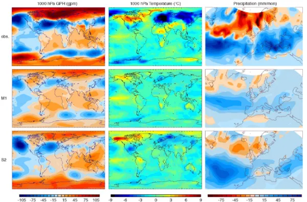
Figure 1 displays observed anomalies of temperature and GPH at 1000 hPa as well as precipitation for January to March 1987 and 1989. The two winters exhibit the well known ENSO imprint in the North Pacific area such as a strong (weak) Aleutian low

5

for El Ni ˜no (La Ni ˜na), accompanied by high (low) temperatures in Alaska. Temperature anomalies in northeastern Europe were strongly negative for the El Ni ˜no winter and positive for the La Ni ˜na winter. The 1000 hPa GPH field shows a pronounced neg-ative (positive) NAO pattern in the two winters. This is in excellent agreement with the “canonical” effect of ENSO on Europe in late winter. The El Ni˜no winter also

re-10

sembles the strong 1940-1942 case (Br ¨onnimann et al., 2004). A strong precipitation signal is found especially for the La Ni ˜na winter, with negative anomalies throughout the Mediterranean area and positive anomalies in northwestern Europe. The El Ni ˜no case shows anomalies of opposite sign, but slightly weaker in amplitude. In general, the results show a close to symmetric response for these two winters with respect to most

15

of the features, and they again suggest that 1986–1989 was a “classical” ENSO cycle with respect to its effect on the circulation over the North Atlantic-European sector.

Comparisons between simulations and observations for the two individual winters are not possible in a strict sense (and therefore not shown here) because of the di ffer-ent climatologies used. Nevertheless, it is interesting to note that similar to the

obser-20

vations, both models show a response that is close to symmetric around the respective climatology in the two winters. Model results (ensemble means) are compared to the observations in Fig. 2 in the form of the difference between the El Ni˜no winter (1987) and the La Ni ˜na winter (1989). The amplitudes of the anomalies are generally smaller in the ensemble means than in the observations, which is expected due to averaging.

25

The patterns, however, are relatively well reproduced by both models. For El Ni ˜no mi-nus La Ni ˜na, all experiments show cold winters in northeastern Europe, stretching all across northern Eurasia, and a dipole pattern in 1000 hPa GPH resembling the

neg-ACPD

Full Screen / Esc

Printer-friendly Version

Interactive Discussion ative mode of the NAO (see Compo et al., 2001, for a discussion of related changes

in subseasonal variability). In the SOCOL experiments as well as in the observations (but not in M1) the anomaly centres lie close to Iceland and the Azores.

For precipitation (Fig. 2), all experiments reproduce the observed decrease in Nor-way and the increase in the Mediterranean area. The precipitation signal over the

5

Atlantic reflects a southward shift in the Atlantic storm track for El Ni ˜no relative to La Ni ˜na, which was also shown by Compo and Sardeshmukh (2004). As for the other fields, the magnitudes of the precipitation anomalies is underestimated. Nevertheless, in all three fields (temperature, GPH, and precipitation) the main differences between El Ni ˜no and La Ni ˜na found in the observations are also statistically significant (t-test,

10

p<0.05) in the model experiments.

Several features, on the other hand, are not well reproduced in the SOCOL model. This concerns in particular surface air temperature over the sea ice north of Alaska (also in MRF9). Also, the warming signal for El Ni ˜no minus La Ni ˜na stretching from Sudan to the Middle East is not well reproduced (again by both models).

15

In addition to the significance of the ensemble mean differences, it is advisable also to look at the distribution functions (see also Melo-Goncalvez et al., 2005). Figure 3 shows histograms of temperatures at a grid point near Dalarna, Sweden (60◦N/15◦E), which is close to the location of the maximum 1000 hPa temperature difference in the observations (note, however, that the grid point is close to the Baltic Sea, where SSTs

20

were prescribed). In order to obtain a larger sample we merged S1 and S2, which show a similar mean response, into one figure. First of all, it becomes obvious that the models differ both with respect to absolute values as well as variability. The surface temperature is lower in SOCOL compared to MRF9. On the other hand, the variability is much higher in SOCOL than in MRF9. The observed temperatures are indicated

25

as coloured lines. Here we use both ERA40 and NCEP/NCAR reanalysis data. They are within the ensemble spread only for SOCOL (S1+S2) in the winter 1987, but out-side the ensemble spread in all other cases. While the models reproduce the sign of the difference between the two winters, they clearly underestimate the magnitude.

ACPD

Full Screen / Esc

Printer-friendly Version

Interactive Discussion

EGU However, it should be noted that the two observation-based data sets (i.e., two

de-pictions of the same “realisation”) also show quite substantial differences and that the observed magnitude amounts to 8–10◦C. This is extreme for a 3-month average. In fact, long temperature records from nearby stations sites (not shown) indicate that the two winters were both close to the record minima and maxima, respectively.

5

With respect to the interpretation of ensemble means, it is clear that the modelled temperature signal shown in Fig. 2 does not arise from a few outliers, nor does it mask a bimodal behaviour. MRF9 seems to show a slightly skewed distribution (longer tail towards low temperatures) for La Ni ˜na, but this feature is not robust when analysing nearby grid cells.

10

3.2 Stratospheric dynamics and chemistry

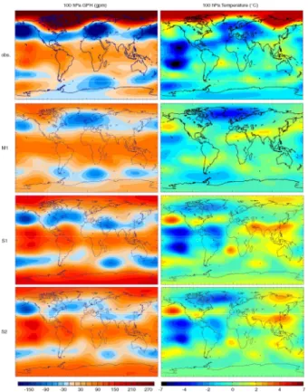
In the following, we focus on the stratospheric dynamics and chemistry. Figure 4 dis-plays the results for GPH and temperature at 100 hPa, representing the lowermost stratosphere. For El Ni ˜no minus La Ni ˜na, temperatures were low and GPH high above the eastern tropical Pacific (see also Claud et al., 1999). At midlatitudes, a clear wave

15

structure is visible in the 100 hPa GPH field, with its main anomaly centres in the North Pacific and central Europe. Temperatures were high over northern Eurasia, but low over the North Atlantic, similar as in the case of the 1940–1942 El Ni ˜no (Br ¨onnimann et al., 2004). The main feature at high latitudes is a weak and meridionally expanded polar vortex, which is consistent with statistical analyses (van Loon and Labitzke, 1987) and

20

model studies (Sassi et al., 2004; Manzini et al., 2006) and again similar to the 1940– 1942 case (Br ¨onnimann et al., 2004). In line with a weak polar vortex and again in agreement with the above mentioned studies, ERA40 temperatures were much higher in 1987 compared to 1989 over much of the Arctic. This is in part due to a major warming in January 1987.

25

The models reproduce the patterns in tropical temperature and GPH anomalies fairly well. MRF9 underestimates the magnitudes in both fields, whereas SOCOL slightly overestimates the GPH response. Both models also show a similar wave-structure

ACPD

Full Screen / Esc

Printer-friendly Version

Interactive Discussion as the observations in temperature and GPH over the North American-Pacific sector.

Further downstream, over the North Atlantic, the wave-pattern is shifted westward in the models compared with the observations. The cooling over the North Atlantic is pronounced and significant in M1 and S2. In the high Arctic, however, the observed temperature signal is not well reproduced in the ensemble means. No significant effect

5

is found except over eastern Siberia. The weak polar vortex in 100 hPa GPH is better reproduced, with a statistically significant signal in all ensemble sets. However, the magnitude is again smaller than in the observations, especially in the MRF9 model. The fact that even MRF9 with a low model top shows a significantly weaker polar vortex confirms that this is a very robust part of the stratospheric ENSO signal.

10

This is not similarly true for stratospheric temperatures, as is discussed in more detail in the following. We analysed the zonal mean signal in temperature, zonal wind, ozone, and EP flux as a function of latitude and altitude. This was done only for the SOCOL model, but not for MRF9, which due to its low model top is not expected to realistically reproduce processes related to wave-mean flow interaction in the middle stratosphere.

15

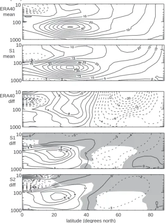
Figures 5 and 6 show zonal mean zonal wind and temperature as a function of latitude and altitude. In addition to the differences between 1987 and 1989, their mean value is also shown for S1 for the comparison of absolute values (S1 and S2 are almost identical with respect to the mean value). SOCOL reproduces the structure as well as the magnitude of the zonal wind fairly well at all levels from the surface up to the

20

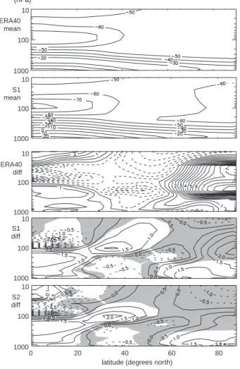
middle stratosphere. The structure of the zonal mean temperature (Fig. 6) is also well reproduced, but absolute values are too low in the tropopause region and in the polar vortex. The differences between El Ni˜no and La Ni˜na agree well with the observations in a qualitative sense. In the zonal winds (Fig. 5) both simulations (S1 and S2) show a stronger subtropical jet and a weakened polar vortex (more so in S1 than S2), which

25

is very similar to the ENSO signal found in statistical analyses of reanalysis data (e.g., Chen et al., 2003). Note that the subtropical jet is displaced southward in the models during El Ni ˜no compared with La Ni ˜na, but not in the observations. The magnitudes of the anomalies also agree well in the troposphere, but in the stratosphere they are

ACPD

Full Screen / Esc

Printer-friendly Version

Interactive Discussion

EGU clearly too small in both simulations, especially in the middle stratosphere. Significance

is limited to the lowermost stratosphere and troposphere.

A similar result is found for the zonal mean temperature differences between El Ni˜no and La Ni ˜na (Fig. 6). The observations show a pronounced signal in the Arctic lower stratosphere. In S1, the pattern is well reproduced, but not its strength, whereas in

5

S2 the pattern is less well reproduced. The Arctic temperature response in the model is significant below 200 hPa. At higher levels, within-ensemble variability is too large for obtaining significant results. Both S1 and S2 show a significant warming of the subtropical tropopause and lower stratosphere which is not seen in the observations. This is probably related to the southward displacement of the subtropical jet in the

10

model (Fig. 5) that is not seen in the observations.

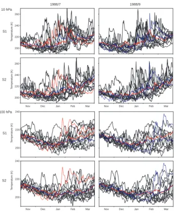
In order to understand the modelled Arctic temperature response in the stratosphere, we analysed 12-hourly series of temperature at the North Pole (10 hPa and 100 hPa) in the individual ensemble members as well as in ERA40 (Fig. 7). The reanalysis data for 1986/87 show a strong disturbance (major midwinter warming) in January. While

15

at 10 hPa, temperatures dropped again during February and reached very low values in March, the disturbance at 100 hPa persisted into spring. In 1988/89, in contrast, the polar stratosphere was undisturbed and cold well into February, but the final warm-ing then was very pronounced. In the SOCOL experiments major warmwarm-ings appear in most of the simulations in both winters, sometimes already in late November or

Decem-20

ber. The large day-to-day variability causes a large within-ensemble variability, which hampers the statistical analysis of ensemble means.

In addition to zonal wind and temperature we also analysed the EP flux as a mea-sure of the planetary-wave driving of the stratospheric circulation. Figure 8 shows zonal means of the upward and meridional components of the EP flux as well as its

diver-25

gence, again for the mean of the two winters and their difference (note that we have averaged EP flux from November to February, thus allowing a four-to-eight week lead with respect to the temperature, zonal wind, and ozone). For the mean values, the EP flux shows an excellent agreement with observations with respect to vertical and

latitu-ACPD

Full Screen / Esc

Printer-friendly Version

Interactive Discussion dinal structure as well as absolute values. This does not only hold for the divergence

of the EP flux, but also for its vertical and meridional components. The differences between El Ni ˜no and La Ni ˜na are also well reproduced. The observations show a neg-ative anomaly in EP flux divergence in most of the extratropical stratosphere, which is also found in both sets of simulations. An analysis of the EP flux components implies

5

two contributions: an increase in the vertical component as well as an increase (in the lower stratosphere) of the poleward component of the EP flux. For both components the anomalies are again well reproduced by both sets of simulations.

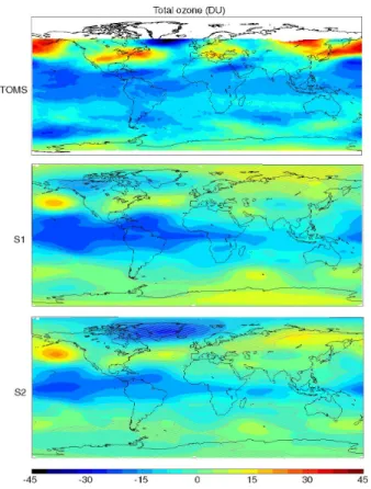
Further comparisons were performed with respect to ozone. The simulated total ozone difference (January-to-March average, El Ni˜no minus La Ni˜na, Fig. 9) shows a

10

very good agreement with TOMS observations with respect to the main structure in the tropics and midlatitudes. Total ozone was reduced over the tropics, especially the tropical Pacific, but enhanced over the midlatitudes with a pronounced imprint of the planetary wave structure. These main features are also significant in the model simu-lations, though underestimated in the ensemble mean. A similar tropical ENSO pattern

15

was also found in other analyses of TOMS data and chemical climate models (e.g., Steinbrecht et al., 2005). Over the polar region (where no TOMS data are available) S1 shows an increase and S2 a decrease in total ozone, but neither is significant.

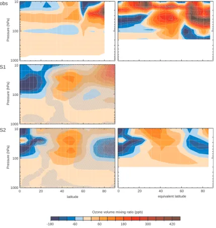
We also analysed the zonal mean vertical distribution of ozone in the SOCOL model and compared it to SAGE II data (Fig. 10, left). Prominent features in the observations

20

are high concentrations in the midlatitude lower stratosphere and in the polar vortex and low ozone concentrations in the tropical middle stratosphere. Both S1 and S2 also show an ozone decrease in the tropical stratosphere, but more pronounced and through the entire lower and middle stratosphere. The midlatitude signal is well repro-duced both with respect to altitude and magnitude of the signal. These anomalies are

25

all statistically significant in the ensemble means. However, the ozone increase in the polar middle stratosphere is only reproduced by S1 and is not significant.

In order to obtain a better picture of the ozone anomalies at middle and high lati-tudes we plotted ozone differences as a function of equivalent latitudes (Fig. 10, right).

ACPD

Full Screen / Esc

Printer-friendly Version

Interactive Discussion

EGU This allows focussing on the effects of chemistry and of the meridional circulation by

removing the planetary wave imprint (which, as discussed above, is well reproduced by SOCOL). CATO was used as the corresponding observational data set. The trans-formation to the equivalent latitude coordinates was only possible for S2, which, as discussed above, fits worse with the observations in the stratosphere than S1. The El

5

Ni ˜no minus La Ni ˜na difference in CATO is larger than in the SAGE II data and shows a different vertical structure of the signal in the tropics and in the subtropical middle stratosphere. The most pronounced feature is again the ozone increase poleward of 65◦equivalent latitude (which is not reproduced by S2), providing clear evidence for a strong ozone increase in the Arctic lower stratosphere. Outside the Arctic the

agree-10

ment between S2 and CATO is relatively good. This concerns especially the tropical lower stratosphere, the subtropical middle stratosphere, and the midlatitude strato-sphere. Hence, even after removing the (well reproduced) planetary wave imprint from the zonal mean ozone field, S2 agrees well with observation-based data except for the Arctic.

15

4 Discussion

At the Earth’s surface, SOCOL reproduced the main anomalies of the two winters 1987 and 1989 relatively well with respect to most analysed features, even though the mag-nitudes of the anomalies are underestimated. Most importantly, both analysed models reproduced the changes in the circulation over the Pacific-North American and North

20

Atlantic-European sectors, i.e., a strengthened Aleutian low and weakened Icelandic low, which is important with respect to the stratospheric signal (Br ¨onnimann et al., 2004). The model results are in good agreement with studies performed with other models (e.g., Mathieu et al., 2004). Note that the results do not imply a causal relation-ship between the extratropical anomalies and ENSO, as SST fields were prescribed

25

globally. For the same reasons, care should be taken when drawing conclusions on predictability (see van Oldenborgh, 2005). What would be necessary to address these

ACPD

Full Screen / Esc

Printer-friendly Version

Interactive Discussion issues are sensitivity experiments prescribing only the tropical or only the Indo-Pacific

SSTs and setting the remaining SSTs to climatology (or using a mixed-layer ocean), which is beyond the scope of this paper.

However, the model simulations and comparison with observations do allow con-clusions with respect to the processes behind ENSO effects on the stratosphere and

5

stratosphere-troposphere coupling, given the consistent tropospheric ENSO response. SOCOL reproduced the observed anomalies of lower stratospheric temperature, GPH as well as total ozone in the tropics. This is the typical ENSO pattern that is directly related to the longitudinal shift of the region of intense atmospheric convection (Hat-sushika and Yamazaki, 2001). All sets of simulations also reproduced the planetary

10

wave imprint in the midlatitude lower stratosphere that appears in the fields of GPH, total ozone (in SOCOL), and to some extent temperature.

Of special interest with respect to the polar stratosphere are the features that are supposedly caused by wave-mean flow interaction. Br ¨onnimann et al. (2004) sug-gested that El Ni ˜no (relative to La Ni ˜na) increases the planetary wave activity

propa-15

gating from the troposphere to the stratosphere (see also Sassi et al., 2004; Manzini et al., 2006). Increased upward propagating planetary wave activity, which accompanies the negative NAO mode, is expected to lead to a weak polar vortex, higher tempera-ture of the Arctic stratosphere in spring, and more major midwinter warmings (Taguchi and Hartmann, 20061). At the same time, the meridional circulation is expected to be

20

strengthened, transporting more ozone from the tropical source regions to the extrat-ropics, which would lead to higher ozone column at mid latitudes and especially in the polar vortex, where the descent is enhanced (see Randel et al., 2002). In addition, re-duced chemical ozone depletion (because of the warmer temperatures) would further increase the Arctic ozone column (Sassi et al., 2004).

25

The observations are in very good agreement with this hypothesis. They not only ex-hibit all of the features discussed above (for El Ni ˜no minus La Ni ˜na a weak and warm polar vortex, a major midwinter warming, more ozone at mid latitudes and in the polar vortex and less ozone, in the tropics, most pronounced in the CATO data), but also

ACPD

Full Screen / Esc

Printer-friendly Version

Interactive Discussion

EGU show anomalous EP flux convergence in the stratosphere, which indicates

strength-ened planetary-wave driving. The SOCOL model reproduces most of these features and hence compares reasonably well, at least qualitatively, with the observations and with other modelling studies (see e.g., Sassi et al., 2004; Manzini et al., 2006). How-ever, the signal in the stratosphere, especially in the middle stratosphere and in the

5

polar vortex, is too weak when compared with observations and some of the prominent features in the observations that are supposedly caused by ENSO are not significant in the ensemble mean.

The agreement between S1, S2, and observations is very good for the components and the divergence of the EP flux. This result implies that the observed and modelled

10

weakening of the polar vortex during El Ni ˜no is largely due to wave-mean flow inter-action (see also Manzini et al., 2006). It is interesting to note that not only the vertical component of the EP flux (and thus the amount of wave energy that reaches the strato-sphere) contributes, but also the meridional component (and thus the degree to which this wave energy is refracted poleward). This is in agreement with the results of Chen

15

et al. (2003) who distinguish between two modes of interannual EP flux variability: a tropospheric mode that is strongly related to the Northern Annular Mode (or NAO) and controls upward propagation of planetary wave energy as well as a stratospheric mode which is strongly related to ENSO and the Pacific North American pattern and controls the poleward refraction of wave energy. The modes are defined as a tropospheric and

20

stratospheric dipole in the anomaly field of EP flux divergence, respectively (see Chen et al., 2003). Both dipoles also appear in the difference field of EP flux divergence in the ERA40 reanalysis and, somewhat less clear, in S1 and S2 (Fig. 8). Thus, in the “canonical” ENSO case, both patterns contribute.

With respect to ozone, all of the above results suggest a strengthening of the

Brewer-25

Dobson circulation that leads to low ozone concentrations in the tropical lower strato-sphere and high concentrations at mid latitudes and in the polar lower stratostrato-sphere (see also Sassi et al., 2004; Pyle et al., 2005). The chemical contribution at high lati-tudes has the same sign as the dynamical contribution, but is dependent on

tempera-ACPD

Full Screen / Esc

Printer-friendly Version

Interactive Discussion ture and therefore probably underestimated by SOCOL. At midlatitudes, the planetary

wave imprint in total ozone is important and is well reproduced by the model.

5 Conclusions

The main anomalies in atmospheric circulation and ozone observed during the “canon-ical” ENSO cycle 1986–1989 were successfully reproduced with the chemical climate

5

model SOCOL. While some deficiencies could be identified with respect to the middle stratosphere, the ENSO signal in surface climate, especially the circulation over the North Atlantic-European region, as well as the imprint in the lower stratosphere agree well with observations. As such, the results provide insight into the mechanisms re-lating ENSO to stratospheric circulation changes. They suggest that both the upward

10

and poleward components of anomalous EP flux are important for obtaining the strato-spheric ENSO signal and that an increase in strength of the Brewer-Dobson circulation during El Ni ˜no is part of that signal.

Acknowledgements. S. Br ¨onnimann was funded by the Swiss National Science Foundation,

A. Fischer is funded by ETH Z ¨urich (TH project CASTRO). GPCP data were obtained via

15

NOAA/CIRES-CDC. We thank G. Compo and P. Sardeshmukh for providing the MRF9 sim-ulations, NASA for providing TOMS and SAGE II data, and I. Wohltmann for providing data and support for the calculation of EP fluxes. ECMWF ERA-40 data used in this study have been provided by ECMWF.

References

20

Adler, R. F., Huffman, G. J., Chang, A., Ferraro, R., Xie, P., Janowiak, J., Rudolf, B., Schneider, U., Curtis, S., Bolvin, D., Gruber, A., Susskind, J., and Arkin, P.: The Version 2 Global Precipitation Climatology Project (GPCP) monthly precipitation analysis (1979–Present), J. Hydrometeorol., 4, 1147–1167, 2003.

ACPD

Full Screen / Esc

Printer-friendly Version

Interactive Discussion

EGU

Alexander M. A., Blad ´e, I., Newmann, M., Lanzante, J. R., Lau, N.-C., and Scott, J. D.: The atmospheric bridge: The influence of ENSO teleconnnections on air-sea interaction over the global oceans, J. Climate, 15, 2205–2231, 2002.

Ambaum, M. H. P. and Hoskins, B. J.: The NAO troposphere-stratosphere connection, J. Cli-mate, 15, 1969–1978, 2002.

5

Andrews, D. G., Holton, J. R., and Leovy, C. B.: Middle Atmosphere Dynamics, Academic Press, 1987.

Baldwin, M. P. and Dunkerton, T. J.: Stratospheric harbingers of anomalous weather regimes, Science, 294, 581–584, 2001.

Br ¨onnimann, S., Luterbacher, J., Staehelin, J., Svendby, T. M., Hansen, G., and Svenøe, T.:

10

Extreme climate of the global troposphere and stratosphere 1940–1942 related to El Ni ˜no, Nature, 431, 971–974, 2004.

Brunner, D., Staehelin, J., Kuensch, H. R., and Bodeker, G. E.: A Kalman filter reconstruction of the vertical ozone distribution in an equivalent latitude – potential temperature framework from TOMS/GOME/SBUV total ozone observations, J. Geophys. Res., in press, 2006.

15

Chen, W., Takahashi, M., and Graf, H.-F.: Interannual variations of planetary wave activity in the northern winter troposphere and stratosphere and their relations to NAM and SST, J. Geophys. Res., 108, 4797, doi:10.1029/2003JD003834, 2003.

Claud, C., Scott., N. A., and Chedin, A.: Seasonal, interannual and zonal temperature variability of the tropical stratosphere based on TOVS satellite data: 1987–1991, J. Climate, 12, 540–

20

550, 1999.

Compo, G. P., Sardeshmukh, P. D., and Penland, C.: Changes of subseasonal variability asso-ciated with El Ni ˜no, J. Climate, 14, 3356–3374, 2001.

Egorova, T. A., Rozanov, E. V., Zubov, V. A., and Karol, I. L.: Model for Investigating Ozone Trends (MEZON), Izvestiya, Atmos. Oceanic Phys., 39, 277–292, 2003.

25

Egorova, T., Rozanov, E., Zubov, V., Manzini, E., Schmutz, W, and Peter, T.: Chemistry-climate model SOCOL: a validation of present-day climatology, Atmos. Chem. Phys., 5, 1577–1576, 2005.

Fraedrich, K.: An ENSO impact on Europe? A review, Tellus, 46A, 541–552, 1994.

Fraedrich, K. and M ¨uller, K.: Climate anomalies in Europe associated with ENSO extremes,

30

Int. J. Climatol., 12, 25–31, 1992.

Giorgetta, M. A.: Der Einfluss der quasi-zweijaehrigen Oszillation auf die allgemeine Zirkula-tion: Modellrechnungen mit ECHAM4, Examensarbeit Nr. 40, Universit ¨at Hamburg,

Ham-ACPD

Full Screen / Esc

Printer-friendly Version

Interactive Discussion

burg, Germany, 1996.

Gouirand, I. and Moron, V.: Variability of the impact of El Ni ˜no-southern oscillation on sea-level pressure anomalies over the North Atlantic in January to March (1874–1996), Int. J. Climatol., 23, 1549–1566, 2003.

Fouquart, Y. and Bonnel, B.: Computations of solar heating of the Earth’s atmosphere: A new

5

parameterization, Beitr. Phys. Atmos., 53, 35–62, 1980.

Hartmann, D. L., Wallace, J. M., Limpasuvan, V., Thompson, D. W. J., and Holton, J. R.: Can ozone depletion and greenhouse warming interact to produce rapid climate change?, Proc. Nat. Acad. Sci., 97, 1412–1417, 2000.

Hatsushika, H. and Yamazaki, K.: Interannual variations of temperature and vertical motion at

10

the tropical tropopause associated with ENSO, Geophys. Res. Lett., 28, 2891–2894, 2001. Hoerling, M. P., Blackmon, M. L., and Ting, M.: Simulating the atmospheric response to the

1985–1987 El Ni ˜no cycle, J. Climate, 5, 669–682, 1992.

Kistler, R., Kalnay, E., Collins, W., et al.: The NCEP-NCAR 50-year reanalysis: Monthly means CD-ROM and documentation, B. Amer. Meteorol. Soc., 82, 247–267, 2001.

15

Kousky, V. E. and Leetma, A.: The 1986–87 Pacific warm episode: Evolution of oceanic and atmospheric anomaly fields, J. Climate, 2, 254–267, 1989.

Kumar, A., Hoerling, M. P., Ji, M., Leetma, A., and Sardeshmukh, P.: Assessing a GCM’s suitability for making seasonal predictions. J. Climate, 9, 115–129, 1996.

Manzini, E., McFarlane, N. A., and McLandress, C.: Impact of the Doppler Spread

Parameteri-20

zation on the simulation of the middle atmosphere circulation using the MA/ECHAM4 general circulation model, J. Geophys. Res., 102, 25 751–25 762, 1997.

Manzini, E., Giorgetta, M. A., Esch, M., Kornblueh, L., and Roeckner, E.: The influence of sea surface temperatures on the Northern winter stratosphere: Ensemble simulations with the MAECHAM5 model, J. Climate, in press, 2006.

25

Mariotti, A., Zeng, N., and Lau, K.-M.: Euro-Mediterranean rainfall and ENSO – a seasonally varying relationship, Geophys. Res. Lett., 29, 1621, doi:10.1029/2001GL014248, 2002. Mathieu, P. P., Sutton, R. T., Dong, B. W., and Collins, M.: Predictability of winter climate over

the North Atlantic European region during ENSO events, J. Climate, 17, 1953–1974, 2004. McPhaden, M. J., Hayes, S. P., and Mangum, L. J.: Variability in the Western equatorial Pacific

30

Ocean during the 1986/87 El Ni ˜no/Southern Oscillation event, J. Phys. Oceanogr., 20, 190– 208, 1990.

Oscil-ACPD

Full Screen / Esc

Printer-friendly Version

Interactive Discussion

EGU

lation sensitivity to the El Ni ˜no/Southern Oscillation polarity in a large-ensemble simulation, Clim. Dyn., 24, 599–606, 2005.

Merkel, U. and Latif, M.: A high resolution AGCM study of the El Ni ˜no impact on the North At-lantic/European sector, Geophys. Res. Lett., 29, 1291, doi:10.1029/2001GL013726, 2002. Miller, L., Cheney, R., and Douglas, B. C.: GEOSAT altimeter observations of Kelvin waves and

5

the 1986–87 El Ni ˜no, Science, 239, 52–54, 1988.

Morcrette, J. J.: Radiation and cloud radiative properties in the European Center for Medium-Range Weather Forecasts forecasting system, J. Geophys. Res., 96, 9121–9132, 1991. Moron, M. and Plaut, G.: The impact of El Ni ˜no Southern Oscillation upon weather regimes

over Europe and the North Atlantic boreal winter, Int. J. Climatol., 23, 363–379, 2003.

10

Palmer, T. N. and Anderson, D. L. T.: Scientific assessment of the prospect of seasonal fore-casting: a European perspective, ECMWF Technical report, 70, 1993.

Pyle, J. A., Braesicke, P., and Zeng, G.: Dynamical variability in the modelling of chemistry– climate interactions, Faraday Discuss., 130, 27–39, 2005.

Pozo-V ´azquez, D., G ´amiz-Fortis, S. R., Tovar-Pescador, J., Esteban-Parra, M. J., and

Castro-15

D´ıez, Y.: North Atlantic winter SLP anomalies based on the autumn ENSO state, J. Climate,

18, 97–103, 2005.

Randel, W. J., Wu, F., and Stolarski, R.: Changes in column ozone correlated with the strato-spheric EP flux, J. Meteorol. Soc. Jpn., 80, 849–862, 2002.

Rozanov, E. V., Schlesinger, M. E., Zubov, V. A., Yang, F., and Andronova, N. G.: The UIUC

20

three-dimensional stratospheric chemical transport model: Description and evaluation of the simulated source gases and ozone, J. Geophys. Res., 104, 11 755–11 781, 1999.

Rozanov, E., Schraner, M., Schnadt, C., Egorova, T., Wild, M., Ohmura, A., Zubov, V., Schmutz, W., and Peter, T.: Assessment of the ozone and temperature variability during 1979–1993 with the chemistry-climate model SOCOL, Adv. Space Res., 35, 1375–1384, 2005.

25

Sardeshmukh, P. D., Compo, G. P., and Penland, C.: Changes of probability associated with El Ni ˜no, J. Climate, 13, 4268–4286, 2000.

Sassi, F., Kinnison, D., Boville, B. A., Garcia, R. R., and Roble, R.: Effect of El Ni˜no-Southern

Oscillation on the dynamical, thermal, and chemical structure of the middle atmosphere, J. Geophys. Res., 109, D17108, doi:10.1029/2003JD004434, 2004.

30

Sato, M., Hansen, J., McCormick, M. P., and Pollack, J. B.: Stratospheric aerosol optical depths, 1850–1990, J. Geophys. Res., 98, 22 987–22 994, 1993.

ACPD

Full Screen / Esc

Printer-friendly Version

Interactive Discussion

Matthes, S., Schnadt, C., Steil, B., and Winkler, P.: Interannual variation patterns of total ozone and lower stratospheric temperature in observations and model simulations, Atmos. Chem. Phys., 6, 349–374, 2006.

Thomason, L. W. and Peter, T.: The Assessment of Stratospheric Aerosol Properties, SPARC Newsletter, 26, 38–39, 2006.

5

Uppala, S. M., K ˚allberg, P. W., Simmons, A. J., et al.: The ERA40 re-analysis. Q. J. R. Meteorol. Soc., 131, 2961–3012, 2005.

van Loon, H. and Labitzke, K.: The Southern Oscillation. Part V: The anomalies in the lower stratosphere of the Northern Hemisphere in winter and a comparison with the Quasi-Biennial Oscillation. Mon. Wea. Rev., 115, 357–369, 1987.

10

van Oldenborgh, G. J.: Comment on “Predictability of winter climate over the North Atlantic European region during ENSO events” by Mathieu, P.-P., Sutton, R. T., Dong, B., and Collins, M., J. Climate, 18, 2770–2772, 2005.

Wu, A. and Hsieh, W. W.: The nonlinear association between ENSO and the Euro-Atlantic winter sea level pressure, Clim. Dyn., 23, 859–868, 2004.

ACPD

Full Screen / Esc

Printer-friendly Version

Interactive Discussion

EGU

Table 1. Overvew of the model experiments.

Run SSTs Description Resolution/top (hPa) No. M0 Climatological Nov–March MRF9 reference T40L18/50 90 M1 Nov–March 1986/87 and 1988/89 MRF9 ENSO T40L18/50 2×45 S0 Transient (1975–2000) SOCOL reference T30L39/0.01 1 S1 Sep–March 1986/87 and 1988/89 SOCOL ENSO T30L39/0.01 2×11 S2 Sep–March 1986/87 and 1988/89 SOCOL ENSO (modified model) T30L39/0.01 2×11

ACPD

Full Screen / Esc

Printer-friendly Version

Interactive Discussion 1000 hPa GPH (gpm) 1000 hPa Temperature (°C) Precipitation (mm/mon)

1987 (El Niño) 1989 (La Niña) -5 -3 -1 0 1 3 5 -15 15 -45 45 75 -75 -75 -45 -15 15 45 75

Fig. 1. Observed anomalies of 1000 hPa geopotential height (left) and air temperature (middle)

as well as precipitation (right) for January to March 1987 (top) and January to March 1989 (bottom) with respect to the 1979–2002 period.

ACPD

Full Screen / Esc

Printer-friendly Version

Interactive Discussion

EGU

22 Figure 2. Difference between January to March 1987 (El Niño) and January to March 1989 (La Niña) in 1000 hPa geopotential height (left) and air temperature (middle) as well as precipitation in the observations (top), M1 ensemble mean (middle), and S2 ensemble mean (bottom). Hatched areas are not significantly different from zero (t-test, p<0.05).

Fig. 2. Difference between January to March 1987 (El Ni˜no) and January to March 1989 (La

Ni ˜na) in 1000 hPa geopotential height (left) and air temperature (middle) as well as precipita-tion in the observaprecipita-tions (top), M1 ensemble mean (middle), and S2 ensemble mean (bottom).

Hatched areas are not significantly different from zero (t-test, p<0.05).

ACPD

Full Screen / Esc

Printer-friendly Version Interactive Discussion S1+S2 JFM 1987 S1+S2 JFM 1989 M1 JFM 1987 M1 JFM 1989 0 0 0 0 2 2 5 5 4 4 10 10 6 6 15 15 264 268 272 276 Temperature (K) NCEP NCEP NCEP NCEP ERA ERA ERA ERA

Fig. 3. Histograms of 1000 hPa temperature near Dalarna (Sweden), averaged from January

to March, for S1+S2 and M1 for 1987 (El Ni˜no) and 1989 (La Ni˜na). The blue and red lines give the corresponding values from ERA40 and NCAP/NCAR reanalysis.

ACPD

Full Screen / Esc

Printer-friendly Version

Interactive Discussion

EGU

24 Figure 4. Difference between 1987 and 1989 in temperature (left) and GPH (right) at 100 hPa, averaged from January to March, in ERA40, M1, S1, and S2. Hatched areas are not significantly different from zero (t-test, p<0.05).

Fig. 4. Difference between 1987 and 1989 in temperature (left) and GPH (right) at 100 hPa,

av-eraged from January to March, in ERA40, M1, S1, and S2. Hatched areas are not significantly different from zero (t-test, p<0.05).

ACPD

Full Screen / Esc

Printer-friendly Version Interactive Discussion 100 1000 ERA40 mean S1 mean 10 10 100 1000 ERA40 diff 10 100 1000 S1 diff 10 100 1000 S2 diff 10 100 1000 0 20 40 60 80

latitude (degrees north) (hPa)

Fig. 5. Mean value and difference between 1987 and 1989 in zonal mean zonal wind (m/s),

averaged from January to March, in ERA40, S1, and S2. Shaded areas are not significantly different from zero (t-test, p<0.05).

ACPD

Full Screen / Esc

Printer-friendly Version Interactive Discussion EGU ERA40 mean S1 mean S2 diff 10 100 1000 ERA40 diff 10 100 1000 10 100 1000 S1 diff 10 100 1000 10 100 1000 0 20 40 60 80

latitude (degrees north) (hPa)

Fig. 6. Mean value and difference between 1987 and 1989 in zonal mean temperature (◦C), averaged from January to March, in ERA40, S1, and S2. Shaded areas are not significantly different from zero (t-test, p<0.05).

ACPD

Full Screen / Esc

Printer-friendly Version Interactive Discussion 200 200 200 200 220 220 220 220 240 240 240 240 260 260

Nov Dec Jan Feb Mar Nov Dec Jan Feb Mar

Nov Dec Jan Feb Mar Nov Dec Jan Feb Mar 1986/7 1988/9 10 hPa 100 hPa S1 S2 S1 S2 T emper ature (K) T emper ature (K) T emper ature (K) T emper ature (K)

Fig. 7. 12-hourly temperature at 10 hPa (top four panels) and 100 hPa (bottom four panels) at

the North Pole from November to March in 1986/87 (left) and 1988/89 (right) for S1 and S2. The dotted lines indicate ERA40 data, the coloured lines give the ensemble means (red: 1986/87, blue: 1988/89).

ACPD

Full Screen / Esc

Printer-friendly Version

Interactive Discussion

EGU

meridional component vertical component divergence

0 20 40 60 80 0 20 40 60 80 0 20 40 60 80 1000 1000 1000 100 100 100 10 10 10 pressure (hP a) pressure (hP a) pressure (hP a)

latitude (degrees north) latitude (degrees north) latitude (degrees north)

S1 mean S1 diff S2 diff 1000 1000 100 100 10 10 pressure (hP a) pressure (hP a) ERA40 mean ERA40 diff -1 -1 -10 -10 1 1 -1 -10 100 100 10 1 0.01 0.1 0.1 1 10 -0.1 0.1 -1 -1 -10 -1 -1 -10 -1000 -0.1 -10 -100 10010 100 0.01 0.1 1 -0.1 10 -100 -1000 -1 1 10 10 1 1 -100 100 100 100 0.1 -0.1 1 0.1 -0.1 1 0.1 -1 1 10 10 -1-1 -0.1 10 -10 0.1 1 -0.1 -0.1 100 10 1 -1 100 1 10 -10 -1 -1 0.1 1 -0.1 -0.1 10 1 -0.1 -10 -10

Fig. 8. Mean value and difference between El Ni˜no and La Ni˜na in zonal mean EP flux,

aver-aged from November to February. In ERA40 reanalysis, S1, and S2. Left: poleward

compo-nent, middle: upward component (both given as 106 kg s−2). Right: divergence (kg m−1s−2).

ACPD

Full Screen / Esc

Printer-friendly Version

Interactive Discussion

EGU

Figure 9. Difference between 1987 and 1989 in total ozone, averaged from January to March, in TOMS Version 8 data, S1, and S2. Hatched areas are not significantly different from zero (t-test, p<0.05).

Fig. 9. Difference between 1987 and 1989 in total ozone, averaged from January to March,

in TOMS Version 8 data, S1, and S2. Hatched areas are not significantly different from zero

(t-test, p<0.05).

ACPD

Full Screen / Esc

Printer-friendly Version Interactive Discussion EGU S2 S1 obs 10 100 1000 Pressure (hP a) 10 100 1000 Pressure (hP a) 10 100 1000 Pressure (hP a)

latitude equivalent latitude

Ozone volume mixing ratio (ppb)

0 20 40 60 80 0 20 40 60 80

-180 -60 60 180 300 420

Fig. 10. Difference between 1987 and 1989 in zonal mean ozone mixing ratio as a function of

latitude and altitude, averaged from January to March, in observations (SAGE II and CATO), S1, and S2. Left: geographical latidues, right: equivalent latitudes. Hatched areas are not significantly different from zero (t-test, p<0.05).