The COSMO-LEPS mesoscale ensemble system: validation of the methodology and verification

(1)

HAL Id: hal-00302614

https://hal.archives-ouvertes.fr/hal-00302614

Submitted on 20 May 2005

HAL is a multi-disciplinary open access

archive for the deposit and dissemination of

sci-entific research documents, whether they are

pub-lished or not. The documents may come from

teaching and research institutions in France or

abroad, or from public or private research centers.

L’archive ouverte pluridisciplinaire HAL, est

destinée au dépôt et à la diffusion de documents

scientifiques de niveau recherche, publiés ou non,

émanant des établissements d’enseignement et de

recherche français ou étrangers, des laboratoires

publics ou privés.

The COSMO-LEPS mesoscale ensemble system:

validation of the methodology and verification

C. Marsigli, F. Boccanera, A. Montani, T. Paccagnella

To cite this version:

C. Marsigli, F. Boccanera, A. Montani, T. Paccagnella. The COSMO-LEPS mesoscale ensemble

system: validation of the methodology and verification. Nonlinear Processes in Geophysics, European

Geosciences Union (EGU), 2005, 12 (4), pp.527-536. �hal-00302614�

(2)

Nonlinear Processes in Geophysics, 12, 527–536, 2005 SRef-ID: 1607-7946/npg/2005-12-527

European Geosciences Union

Nonlinear Processes

in Geophysics

The COSMO-LEPS mesoscale ensemble system: validation of the

methodology and verification

C. Marsigli, F. Boccanera, A. Montani, and T. Paccagnella

ARPA-SIM, Bologna, Italy

Received: 21 September 2004 – Revised: 4 April 2005 – Accepted: 26 April 2005 – Published: 20 May 2005 Part of Special Issue “Quantifying predictability”

Abstract. The limited-area ensemble prediction system COSMO-LEPS has been running every day at ECMWF since November 2002. A number of runs of the non-hydrostatic limited-area model Lokal Modell (LM) are available every day, nested on members of the ECMWF global ensemble. The limited-area ensemble forecasts range up to 120 h and LM-based probabilistic products are disseminated to several national and regional weather services. Some changes of the operational suite have recently been made, on the basis of the results of a statistical analysis of the methodology. The anal-ysis is presented in this paper, showing the benefit of increas-ing the number of ensemble members. The system has been designed to have a probabilistic support at the mesoscale, fo-cusing the attention on extreme precipitation events. In this paper, the performance of COSMO-LEPS in forecasting pre-cipitation is presented. An objective verification in terms of probabilistic indices is made, using a dense network of obser-vations covering a part of the COSMO domain. The system is compared with ECMWF EPS, showing an improvement of the limited-area high-resolution system with respect to the global ensemble system in the forecast of high precipitation values. The impact of the use of different schemes for the parametrisation of the convection in the limited-area model is also assessed, showing that this have a minor impact with respect to run the model with different initial and boundary condition.

1 Introduction

The forecast of severe weather events is still a challenging problem. The key role played by mesoscale and orographic-related processes can seriously limit the predictability of

intense and localised events. Although the use of

high-resolution limited-area models (LAMs) has improved the short-range prediction of locally intense events, it is

some-Correspondence to: C. Marsigli

(cmarsigli@smr.arpa.emr.it)

times difficult to forecast accurately their space-time evolu-tion, especially for ranges longer than 48 h. In the recent years, many weather centres have given more and more em-phasis to the probabilistic approach (Tracton and Kalnay, 1993; Molteni et al., 1996; Houtekamer et al., 1996), which has proved to be an important tool to tackle the predictability problem beyond day 2. Nevertheless, global ensemble sys-tems are usually run at a relatively low horizontal resolution (80 km at most), making difficult their use where the forecast of severe and localised weather events is concerned. With re-gard to the use of limited-area models within ensemble sys-tems, ARPA-SIM (the Regional Hydro-Meteorological Ser-vice of Emilia-Romagna, in Italy) developed LEPS (Limited-area Ensemble Prediction System) (Molteni et al., 2001; Marsigli et al., 2001; Montani et al., 2001, 2003a), which after some tests led to the COSMO-LEPS implementation (Montani et al., 2003b).

The LEPS methodology allows us to combine the benefits of the probabilistic approach (a set of different evolution sce-narios is provided to the forecaster) with the high-resolution detail of the LAM integrations, with a limited computational investment. The methodology is based on an algorithm that selects a number of members out of a global ensemble sys-tem. In particular, the 51-member ECMWF EPS (Ensemble Prediction System) is used. The selected ensemble mem-bers (called Representative Memmem-bers, RMs) provide initial and boundary conditions to run a limited-area model.

Following the encouraging results of the early experimen-tal phase, the generation of an “experimenexperimen-tal-operational” limited-area ensemble prediction system, the COSMO-LEPS project, has started in November 2002 on the ECMWF computer system under the auspices of COSMO (Montani et al., 2003b). COSMO (COnsortium for Small-scale MOd-eling, http://www.cosmo-model.org) is a consortium involv-ing Germany, Italy, Switzerland, Greece and Poland which aims to develop, improve and maintain the non-hydrostatic limited-area model Lokal Modell (LM). COSMO-LEPS aims at the development and pre-operational test of a “late-short to early-medium-range” (48–120 h) probabilistic

(3)

fore-528 C. Marsigli et al.: COSMO-LEPS verification

2 C. Marsigli et al.: COSMO–LEPS verification

30°N 30°N 35°N 35°N 40°N 40°N 45°N 45°N 50°N 50°N 55°N 55°N 60°N 60°N 10°W 10°W 5°W 5°W 0° 0° 5°E 5°E 10°E 10°E 15°E 15°E 20°E 20°E 25°E 25°E 30°E 30°E 35°E 35°E

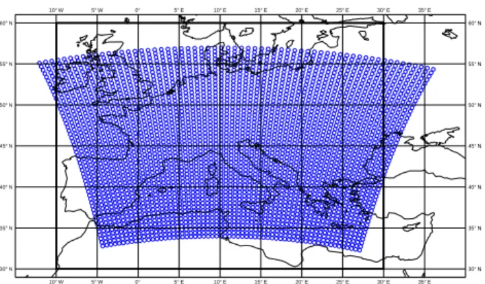
Fig. 1. COSMO–LEPS operational domain (small circles) and

clus-tering area (thick rectangle).

LAM over a domain covering all countries involved in COSMO (Fig. 1).

The methodology can be regarded as a downscaling of the forecasts provided by a global ensemble, aiming at transfer-ring to the probabilistic approach the benefit of the high– resolution. The perturbations are introduced into the limited– area model both through the initial conditions and by means

of the perturbed lateral boundary conditions. The added

value of the system resides in joining the skill of a global ensemble system to depict the possible evolution scenarios with the capability of an high–resolution LAM to describe better local meteorological processes. Perturbations in the initial conditions have not been considered due to two main reasons: the computational burden and the fact that COSMO-LEPS is mainly designed for the medium-range (day 3-5), where the impact of the boundary conditions is regarded to be more relevant. Recently (June 2004) model perturbations have been introduced withing COSMO–LEPS by using two different convection schemes. This was done in order to try to consider a more local source of spread.

The developed methodology makes use of a global ensem-ble size reduction technique in order to avoid to increase too much the computational costs: a price in terms of ensem-ble size is paid in order to save computational time for the high–resolution integrations. The ensemble size reduction is necessary in order to render affordable the integrations of a number of limited–area model runs within a few hours. This permits to have the forecasts issued by the system available in the early morning in the meteorological operation rooms, where its performances can be evaluated by the forecasters in real time.

The extent to which the aim has been reached has been evaluated both with an objective verification, which is pre-sented in this paper, and on a case–study basis. In the above mentioned references and in Marsigli et al. (2004), it has been shown that, over a number of test cases and for sev-eral forecast ranges (48–120 hours), LEPS (the early exper-imental system) and COSMO–LEPS (the real–time quasi– operational system) have shown better performance than EPS for the quantitative forecast of intense precipitation, as well as the geographical localisation of the regions most likely

0h 0h 0h +24h +12h +12h +96h +144h +120h +108h +132h +120h

youngest EPS ready OLDEST EPS MIDDLE EPS YOUNGEST EPS Clustering Times N − 2 N − 1 Starting of LM integrations 1 5 3 M E M B E R S N + 1 N + 2 N + 3 N + 4

COSMO−LEPS products ready

N 12 12 12 12 00 00 00 00 00 00 12 12 12 O

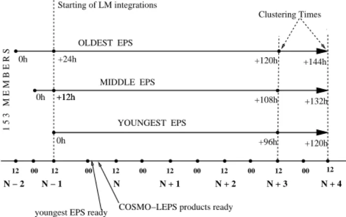
Fig. 2. Details of the COSMO–LEPS suite.

to be affected by the flood events. Then, as regards severe precipitation events, the impact the high–resolution within a probabilistic system seems to be positive.

An objective verification of COSMO–LEPS is being car-ried out at ARPA–SIM, focusing the attention on the precip-itation forecast. Verification aims towards an understanding of the abilities and shortcomings of the system, in order to ameliorate its design and to provide guidelines to the end users (forecasters, civil protection, etc). In this paper, verifi-cation of daily precipitation has been performed over the pe-riod September–November 2003. The probabilistic indices used in this paper are: Brier Skill Score (Wilks , 1995), ROC Curves (Mason and Graham , 1999) and Percentage of Out-liers (Buizza , 1997). With regards to the system configura-tion, the analysis focuses on the methodology that leads to the choice of the Representative Members. This analysis has been performed over the same period.

The paper is organised as follows: in Section 2 the COSMO–LEPS system is described, as it has been since June 2004, while in Section 3 a statistical analysis of the method-ology is presented, leading to a new configuration of the sys-tem. In Section 4 an objective verification of the performance of COSMO–LEPS is carried out, comparing the system with the ECMWF EPS. In Section 5, the COSMO–LEPS is com-pared with a parallel suite in which another scheme for the parametrisation of the precipitating convection is used. Fi-nally, conclusions are drawn in Section 6.

2 The COSMO–LEPS operational system.

The set–up of the COSMO–LEPS suite, as it was when the verification was carried out, is described in this Section. From the beginning of June 2004 the suite has changed, as a consequence of the results obtained in Sect. 3 and in Sect. 5. A Cluster Analysis and Representative Member Selection Algorithm is applied to the ECMWF global ensemble sys-tem. For a description of the Cluster Analysis technique, a technique which permits to separate data into groups whose identity are not known in advance, the reader is referred

Fig. 1. COSMO-LEPS operational domain (small circles) and clus-tering area (thick rectangle).

casting system using a LAM over a domain covering all countries involved in COSMO (Fig. 1).

The methodology can be regarded as a downscaling of the forecasts provided by a global ensemble, aiming at trans-ferring to the probabilistic approach the benefit of the high-resolution. The perturbations are introduced into the limited-area model both through the initial conditions and by means

value of the system resides in joining the skill of a global ensemble system to depict the possible evolution scenarios with the capability of an high-resolution LAM to describe better local meteorological processes. Perturbations in the initial conditions have not been considered due to two main reasons: the computational burden and the fact that COSMO-LEPS is mainly designed for the medium-range (day 3–5), where the impact of the boundary conditions is regarded to be more relevant. Recently (June 2004) model perturbations have been introduced withing COSMO-LEPS by using two different convection schemes. This was done in order to try to consider a more local source of spread.

The developed methodology makes use of a global ensem-ble size reduction technique in order to avoid to increase too much the computational costs: a price in terms of ensem-ble size is paid in order to save computational time for the high-resolution integrations. The ensemble size reduction is necessary in order to render affordable the integrations of a number of limited-area model runs within a few hours. This permits to have the forecasts issued by the system available in the early morning in the meteorological operation rooms, where its performances can be evaluated by the forecasters in real time.

The extent to which the aim has been reached has been evaluated both with an objective verification, which is pre-sented in this paper, and on a case-study basis. In the above mentioned references and in Marsigli et al. (2004), it has been shown that, over a number of test cases and for several forecast ranges (48–120 h), LEPS (the early experimental system) and COSMO-LEPS (the real-time quasi-operational system) have shown better performance than EPS for the quantitative forecast of intense precipitation, as well as the

geographical localisation of the regions most likely to be af-fected by the flood events. Then, as regards severe precipi-tation events, the impact the high-resolution within a proba-bilistic system seems to be positive.

An objective verification of COSMO-LEPS is being car-ried out at ARPA-SIM, focusing the attention on the precip-itation forecast. Verification aims towards an understanding of the abilities and shortcomings of the system, in order to ameliorate its design and to provide guidelines to the end users (forecasters, civil protection, etc). In this paper, ver-ification of daily precipitation has been performed over the period September-November 2003. The probabilistic indices used in this paper are: Brier Skill Score (Wilks, 1995), ROC Curves (Mason and Graham, 1999) and Percentage of Out-liers (Buizza, 1997). With regards to the system configura-tion, the analysis focuses on the methodology that leads to the choice of the Representative Members. This analysis has been performed over the same period.

The paper is organised as follows: in Sect. 2 the COSMO-LEPS system is described, as it has been since June 2004, while in Sect. 3 a statistical analysis of the methodology is presented, leading to a new configuration of the system. In Sect. 4 an objective verification of the performance of COSMO-LEPS is carried out, comparing the system with the ECMWF EPS. In Sect. 5, the COSMO-LEPS is com-pared with a parallel suite in which another scheme for the parametrisation of the precipitating convection is used. Fi-nally, conclusions are drawn in Sect. 6.

2 The COSMO-LEPS operational system

The set-up of the COSMO-LEPS suite, as it was when the verification was carried out, is described in this section. From the beginning of June 2004 the suite has changed, as a con-sequence of the results obtained in Sect. 3 and in Sect. 5.

A Cluster Analysis and Representative Member Selection Algorithm is applied to the ECMWF global ensemble sys-tem. For a description of the Cluster Analysis technique, a technique which permits to separate data into groups whose identity are not known in advance, the reader is referred to Wilks (1995). The Ensemble Prediction System (EPS)

is now based on a TL255L40 model (spectral model with

truncation at wavenumber 255 and 40 vertical levels), corre-sponding to a horizontal resolution of about 80 km, and has 51 members (Molteni et al., 1996; Buizza et al., 1999). Three successive 12-h-lagged EPS runs (started at 12:00 UTC of day N-2, at 00:00 and 12:00 UTC of day N-1) are grouped to-gether so as to generate a 153-member super-ensemble; (see Fig. 2). A hierarchical cluster analysis is performed on the 153 members so as to group all elements into 5 clusters (of different populations); the clustering variables are the geopo-tential height, the two component of the horizontal wind and the specific humidity at three pressure levels (500, 700, 850 hPa) and at two forecast times (fc+96 and fc+120 for the “youngest” EPS, the one started at 12:00 UTC of day N-1);

(4)

C. Marsigli et al.: COSMO-LEPS verification 529

the cluster domain covers the region 30◦_N–60◦_{N, 10}◦_W–

40◦_{E (rectangle in Fig. 1).}

The use of the super-ensemble was introduced (Montani et al., 2003a) aiming at increasing the spread of the global ensemble on which the cluster analysis is performed.

Within each cluster, one representative member (RM) is selected according to the following criteria: the RM is that element closest to the members of its own clusters and most distant from the members of the other clusters; distances are calculated using the same variables and the same metric as in the cluster analysis; hence, 5 RMs are selected. Each RM provides initial and boundary conditions for the integrations with LM, which is run 5 times for 120 h, always starting at 12:00 UTC of day N-1 and ending at 12:00 UTC of day N+4. The LM is run with a horizontal resolution 1x'10 km and with 32 levels in the vertical; the time-step used for the inte-grations is 60 s.

Probability maps based on LM runs are generated by as-signing to each LM integration a weight proportional to the population of the cluster from which the RM (providing ini-tial and boundary conditions) was selected. Deterministic products (that is, the 5 LM scenarios in terms of surface and upper-level fields) are also produced.

The products are disseminated to the COSMO community for evaluation. COSMO-LEPS dissemination started dur-ing November 2002 and, at the time of writdur-ing (September 2004), the system is being tested to assess its usefulness in met-ops rooms, particularly in terms of the assistance given to forecasters in cases of extreme events.

3 Statistical analysis of the methodology

The idea of joining three consecutive EPS to form a super-ensemble is based on the need of enlarging the size of the en-semble on which the RM selection algorithm is applied. This permits an increase in the ensemble spread and a wider part of the phase space spanned by the global ensemble members. Nevertheless, this is obtained by paying a price in terms of skill: the older the EPS, the less skillful their members are. In order to quantify the relative effects of the increased spread and of the decreased skill, the Representative Members sen with the current methodology are compared to those cho-sen using only one or two EPS. The three ensembles that are compared are, then:

– the ensemble made up by the 5 RMs selected applying

the Cluster Analysis and Representative Member Selec-tion Algorithm on the three most recent EPS (referred to “3-EPS”), which is the original operational configu-ration.

the Cluster Analysis and Representative Member Selec-tion Algorithm on the two most recent EPS (referred to “2-EPS”).

the Cluster Analysis and Representative Member

Selec-2 C. Marsigli et al.: COSMO–LEPS verification

30°N 30°N 35°N 35°N 40°N 40°N 45°N 45°N 50°N 50°N 55°N 55°N 60°N 60°N 10°W 10°W 5°W 5°W 0° 0° 5°E 5°E 10°E 10°E 15°E 15°E 20°E 20°E 25°E 25°E 30°E 30°E 35°E 35°E

Fig. 1. COSMO–LEPS operational domain (small circles) and clus-tering area (thick rectangle).

LAM over a domain covering all countries involved in COSMO (Fig. 1).

The methodology can be regarded as a downscaling of the forecasts provided by a global ensemble, aiming at transfer-ring to the probabilistic approach the benefit of the high– resolution. The perturbations are introduced into the limited– area model both through the initial conditions and by means

value of the system resides in joining the skill of a global ensemble system to depict the possible evolution scenarios with the capability of an high–resolution LAM to describe better local meteorological processes. Perturbations in the initial conditions have not been considered due to two main reasons: the computational burden and the fact that COSMO-LEPS is mainly designed for the medium-range (day 3-5), where the impact of the boundary conditions is regarded to be more relevant. Recently (June 2004) model perturbations have been introduced withing COSMO–LEPS by using two different convection schemes. This was done in order to try to consider a more local source of spread.

The developed methodology makes use of a global ensem-ble size reduction technique in order to avoid to increase too much the computational costs: a price in terms of ensem-ble size is paid in order to save computational time for the high–resolution integrations. The ensemble size reduction is necessary in order to render affordable the integrations of a number of limited–area model runs within a few hours. This permits to have the forecasts issued by the system available in the early morning in the meteorological operation rooms, where its performances can be evaluated by the forecasters in real time.

The extent to which the aim has been reached has been evaluated both with an objective verification, which is pre-sented in this paper, and on a case–study basis. In the above mentioned references and in Marsigli et al. (2004), it has been shown that, over a number of test cases and for sev-eral forecast ranges (48–120 hours), LEPS (the early exper-imental system) and COSMO–LEPS (the real–time quasi– operational system) have shown better performance than EPS for the quantitative forecast of intense precipitation, as well as the geographical localisation of the regions most likely

0h 0h 0h +24h +12h +12h +96h +144h +120h +108h +132h +120h

youngest EPS ready OLDEST EPS MIDDLE EPS YOUNGEST EPS Clustering Times N − 2 N − 1 Starting of LM integrations 1 5 3 M E M B E R S N + 1 N + 2 N + 3 N + 4

COSMO−LEPS products ready

N 12 12 12 12 00 00 00 00 00 00 12 12 12 O

Fig. 2. Details of the COSMO–LEPS suite.

to be affected by the flood events. Then, as regards severe precipitation events, the impact the high–resolution within a probabilistic system seems to be positive.

An objective verification of COSMO–LEPS is being car-ried out at ARPA–SIM, focusing the attention on the precip-itation forecast. Verification aims towards an understanding of the abilities and shortcomings of the system, in order to ameliorate its design and to provide guidelines to the end users (forecasters, civil protection, etc). In this paper, verifi-cation of daily precipitation has been performed over the pe-riod September–November 2003. The probabilistic indices used in this paper are: Brier Skill Score (Wilks , 1995), ROC Curves (Mason and Graham , 1999) and Percentage of Out-liers (Buizza , 1997). With regards to the system configura-tion, the analysis focuses on the methodology that leads to the choice of the Representative Members. This analysis has been performed over the same period.

The paper is organised as follows: in Section 2 the COSMO–LEPS system is described, as it has been since June 2004, while in Section 3 a statistical analysis of the method-ology is presented, leading to a new configuration of the sys-tem. In Section 4 an objective verification of the performance of COSMO–LEPS is carried out, comparing the system with the ECMWF EPS. In Section 5, the COSMO–LEPS is com-pared with a parallel suite in which another scheme for the parametrisation of the precipitating convection is used. Fi-nally, conclusions are drawn in Section 6.

2 The COSMO–LEPS operational system.

The set–up of the COSMO–LEPS suite, as it was when the verification was carried out, is described in this Section. From the beginning of June 2004 the suite has changed, as a consequence of the results obtained in Sect. 3 and in Sect. 5. A Cluster Analysis and Representative Member Selection Algorithm is applied to the ECMWF global ensemble sys-tem. For a description of the Cluster Analysis technique, a technique which permits to separate data into groups whose identity are not known in advance, the reader is referred

Fig. 2. Details of the COSMO-LEPS suite.

tion Algorithm on the most recent EPS (referred to “1-EPS”).

This analysis is performed in terms of 24-h precipitation. The forecast values at each grid point are compared with a proxy for the true precipitation occurred chosen as the +24 h forecast by the ECMWF deterministic model. It is not impor-tant the extent to which this proxy is a good approximation for the truth, because this is a comparison among different configuration of the same model. The period chosen for this test is September–November 2003 and the area is the cluster-ing area (rectangle in Fig. 1).

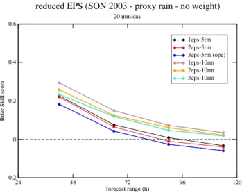
Results show that the Brier Skill Score (the higher the bet-ter) is higher when the clustering is based on the most re-cent EPS only (Fig. 3, black line), while it is lower for the 3-EPS super-ensemble (blue line). The difference between the two is not so remarkable, but it remains at every forecast range. The 2-EPS super-ensemble (red line) has an interme-diate skill, equal to the one of the 1-EPS ensemble at the first and last forecast ranges, its general performance being closer to that of the 1-EPS ensemble. Similar conclusions are drawn when the ROC area scores are considered (not shown).

The percentage of outliers of the systems is also shown. This is the percentage of times the “truth” falls out of the range of the forecast values, so the lower the better. The percentage of outliers (Fig. 4) of the 1-EPS ensemble (black line) is rather higher than the other two, for every forecast range, while there is almost no difference in terms of outliers between the 2-EPS (red line) and the 3-EPS (blue line) en-sembles. These results seem to indicate that the use of just two EPS in the super-ensemble can be a good compromise, permitting a significant decrease in the percentage of outliers but leading to only a small worsening of the skill.

In order to quantify the impact of the ensemble size on the performance of the system, the cluster analysis has been repeated by fixing the number of clusters to 10 and by select-ing, then, 10 Representative Members. This has been done for each of the three ensemble configurations already consid-ered, leading to the three configurations: 3-EPS-10RMs, 2-EPS-10RMs and 1-2-EPS-10RMs. The impact of the ensemble size proves to be quite remarkable; the difference between

(5)

530 C. Marsigli et al.: COSMO-LEPS verification

24 48 72 96 120 forecast range (h) -0,2 0 0,2 0,4 0,6

Brier Skill score

1eps-5rm 2eps-5rm 3eps-5rm (ope) 1eps-10rm 2eps-10rm 3eps-10rm reduced EPS (SON 2003 - proxy rain - no weight)

20 mm/day

Fig. 3. Brier Skill Score as a function of the forecast range for the event precipitation exceeding 20mm/24h relative to the RM EPS. The

different configurations are: 5 clusters algorithm based on 1 EPS (black line), on 2 EPS (red line) and on 3 EPS (operational configuration, blue line); 10 clusters algorithm based on 1 EPS (gray line), on 2 EPS (orange line) and on 3 EPS (cyan line).

24 48 72 96 120 forecast range (h) 0 0,1 0,2 0,3 outliers 1eps-5rm 2eps-5rm 3eps-5rm (ope) 1eps-10rm 2eps-10rm 3eps-10rm

reduced EPS (SON 2003 - proxy rain)

Fig. 4. Percentage of outliers for the RM EPS. The different configurations are: 5 clusters algorithm based on 1 EPS (black line), on 2 EPS

(red line) and on 3 EPS (operational configuration, blue line); 10 clusters algorithm based on 1 EPS (gray line), on 2 EPS (orange line) and on 3 EPS (cyan line).

Fig. 3. Brier Skill Score as a function of the forecast range for the event precipitation exceeding 20 mm/24 h relative to the RM EPS. The different configurations are: 5 clusters algorithm based on 1 EPS (black line), on 2 EPS (red line) and on 3 EPS (operational con-figuration, blue line); 10 clusters algorithm based on 1 EPS (gray line), on 2 EPS (orange line) and on 3 EPS (cyan line).

each 5-member ensemble and the correspondent 10-member ensemble being about 0.1 in terms of Brier Skill Score, for every configuration. This is shown in Fig. 3, where the blue line EPS-5RMs) is to be compared with the cyan line (3-EPS-10RMs), the red line (2-EPS-5RMs) with the orange line (2-EPS-10RMs) and the black line (1-EPS-5RMs) with the brown line (1-EPS-10RMs). The impact of doubling the ensemble size is almost the same for every configuration and is predominant with respect to the impact of changing the number of EPS on which the Cluster Analysis is performed. In terms of Outliers (Fig. 4), it can be seen that doubling the ensemble size greatly reduces the Percentage of Outliers, but, due to the dependence of this measure on the ensemble size, a direct comparison may be not appropriate.

These results led to two major modification of the COSMO-LEPS methodology at the beginning of June 2004: the super-ensemble has been built by using only the 2 most recent EPS and the number of clusters has been fixed to 10 (2-EPS-10RMs configuration), nesting Lokal Modell on each of the so selected 10 RMs.

4 Verification of COSMO-LEPS against the EPS

In order to quantify the added value brought about by the mesoscale probabilistic system, COSMO-LEPS is compared with the EPS. The comparison is made difficult by two main factors: the difference in the number of ensemble members (5 for COSMO-LEPS and 51 for the EPS) and the differ-ence in terms of resolution (10 km for COSMO-LEPS and 80 km for the EPS). As far as the population of the ensem-bles is concerned, COSMO-LEPS is also compared with a small EPS ensemble made up by the 5 Representative

Mem-4 C. Marsigli et al.: COSMO–LEPS verification

24 48 72 96 120 forecast range (h) -0,2 0 0,2 0,4 0,6

Brier Skill score

1eps-5rm 2eps-5rm 3eps-5rm (ope) 1eps-10rm 2eps-10rm 3eps-10rm reduced EPS (SON 2003 - proxy rain - no weight)

20 mm/day

Fig. 3. Brier Skill Score as a function of the forecast range for the event precipitation exceeding 20mm/24h relative to the RM EPS. The

different configurations are: 5 clusters algorithm based on 1 EPS (black line), on 2 EPS (red line) and on 3 EPS (operational configuration, blue line); 10 clusters algorithm based on 1 EPS (gray line), on 2 EPS (orange line) and on 3 EPS (cyan line).

24 48 72 96 120 forecast range (h) 0 0,1 0,2 0,3 outliers 1eps-5rm 2eps-5rm 3eps-5rm (ope) 1eps-10rm 2eps-10rm 3eps-10rm reduced EPS (SON 2003 - proxy rain)

Fig. 4. Percentage of outliers for the RM EPS. The different configurations are: 5 clusters algorithm based on 1 EPS (black line), on 2 EPS

(red line) and on 3 EPS (operational configuration, blue line); 10 clusters algorithm based on 1 EPS (gray line), on 2 EPS (orange line) and

on 3 EPS (cyan line).Fig. 4. Percentage of outliers for the RM EPS. The different

config-urations are: 5 clusters algorithm based on 1 EPS (black line), on 2 EPS (red line) and on 3 EPS (operational configuration, blue line); 10 clusters algorithm based on 1 EPS (gray line), on 2 EPS (orange line) and on 3 EPS (cyan line).

bers. This permits us to quantify the impact of the increased resolution alone. The problem of the very different resolu-tions of the two systems is tackled by upscaling both systems to a lower resolution: the grid point forecasts of both

mod-els are aggregated over boxes of 1.5×1.5◦. For each model,

this was done in two ways: averaging all the forecast values falling into the box or selecting the maximum among all the forecast values falling into the box. The comparison is made in terms of 24-h precipitation, against observed data from a very dense network of raingauges. Precipitation is accumu-lated from 06:00 to 06:00 UTC. In order to properly compare forecast values on grid points and observed values on station points, the observations within a box are treated, as the fore-cast values, in two ways: all the observed values falling into a box are averaged and the obtained value is compared directly with the averaged forecast value or the maximum among all the observed values falling into a box is selected and com-pared with the maximum forecast value. The comparison is carried out over a large area included in the COSMO-LEPS domain, covering Germany, Switzerland and Northern Italy. The dense network of stations recording daily precipitation (about 4000 every day) is shown in Fig. 5.

The three ensemble systems compared are:

– the COSMO-LEPS system, made up of 5 members, 10

km horizontal resolution, referred to as “cleps”;

– the EPS mini-ensemble composed of the 5

Representa-tive Members chosen from the super-ensemble, 80 km horizontal resolution, referred to as “epsrm”;

– the operational 51-member ECMWF EPS starting at

the same initial time as COSMO-LEPS (the “youngest” EPS constituting the super-ensemble), 80 km horizontal resolution, referred to as “eps51”.

(6)

C. Marsigli et al.: COSMO-LEPS verification 531

C. Marsigli et al.: COSMO–LEPS verification 5

tween each 5–member ensemble and the correspondent 10– member ensemble being about 0.1 in terms of Brier Skill Score, for every configuration. This is shown in Fig. 3, where the blue line (3–EPS–5RMs) is to be compared with the cyan line (3–EPS–10RMs), the red line (2–EPS–5RMs) with the orange line (2–EPS–10RMs) and the black line (1– EPS–5RMs) with the brown line (1–EPS–10RMs). The im-pact of doubling the ensemble size is almost the same for every configuration and is predominant with respect to the impact of changing the number of EPS on which the Clus-ter Analysis is performed. In Clus-terms of Outliers (Fig. 4), it can be seen that doubling the ensemble size greatly reduces the Percentage of Outliers, but, due to the dependence of this measure on the ensemble size, a direct comparison may be not appropriate.

These results led to two major modification of the COSMO–LEPS methodology at the beginning of June 2004: the super–ensemble has been built by using only the 2 most recent EPS and the number of clusters has been fixed to 10 (2–EPS–10RMs configuration), nesting Lokal Modell on each of the so selected 10 RMs.

4 Verification of COSMO–LEPS against the EPS.

In order to quantify the added value brought about by the mesoscale probabilistic system, COSMO–LEPS is compared with the EPS. The comparison is made difficult by two main factors: the difference in the number of ensemble members (5 for COSMO–LEPS and 51 for the EPS) and the differ-ence in terms of resolution (10 km for COSMO–LEPS and 80 km for the EPS). As far as the population of the ensembles is concerned, COSMO–LEPS is also compared with a small EPS ensemble made up by the 5 Representative Members. This permits us to quantify the impact of the increased res-olution alone. The problem of the very different resres-olutions of the two systems is tackled by upscaling both systems to a lower resolution: the grid point forecasts of both model are aggregated over boxes of 1.5 x 1.5 degrees. For each model, this was done in two ways: averaging all the forecast values falling into the box or selecting the maximum among all the forecast values falling into the box. The comparison is made in terms of 24–hour precipitation, against observed data from a very dense network of raingauges. Precipitation is accu-mulated from 06 to 06 UTC. In order to properly compare forecast values on grid points and observed values on station points, the observations within a box are treated, as the fore-cast values, in two ways: all the observed values falling into a box are averaged and the obtained value is compared directly with the averaged forecast value or the maximum among all the observed values falling into a box is selected and com-pared with the maximum forecast value. The comparison is carried out over a large area included in the COSMO–LEPS domain, covering Germany, Switzerland and Northern Italy. The dense network of stations recording daily precipitation (about 4000 every day) is shown in Fig. 5.

The three ensemble systems compared are:

39°N 39°N 40°N 40°N 41°N 41°N 42°N 42°N 43°N 43°N 44°N 44°N 45°N 45°N 46°N 46°N 47°N 47°N 48°N 48°N 49°N 49°N 50°N 50°N 51°N 51°N 52°N 52°N 53°N 53°N 54°N 54°N 55°N 55°N 7°E 7°E 9°E 9°E 11°E 11°E 13°E 13°E 15°E 15°E 06-06 fino al 02/09/2003 precipitazione cumulata (mm) 24 h

Fig. 5. Network of station providing 24–hour precipitation (06 UTC to 06 UTC) for the COSMO verification.

– the COSMO–LEPS system, made up of 5 members, 10

km horizontal resolution, referred to as “cleps”;

– the EPS mini–ensemble composed of the 5

Representa-tive Members chosen from the super–ensemble, 80 km horizontal resolution, referred to as “epsrm”;

– the operational 51–member ECMWF EPS starting at

the same initial time as COSMO–LEPS (the “youngest” EPS constituting the super–ensemble), 80 km horizon-tal resolution, referred to as “eps51”;

First, the average observed value of each box, obtained by computing the mean of all the observations falling in a box, is compared with the average forecast value relative to the same box, for each of the three forecasting systems. The Brier Skill Score (Fig. 6) and the ROC area (Fig. 7) for the three systems are shown; for both indices, the higher the better. The event considered here is precipitation exceeding 20 mm / 24 h over 1.5 x 1.5 degree boxes. Since the observed and forecast values are averaged over an area of 1.5 x 1.5 degrees, this threshold detects an intense precipitation.

In terms of Brier Skill Score (Fig. 6) the three lines are rather close together. The BSS values of the full–size 51– member EPS (eps51, green line) are slightly higher than

Fig. 5. Network of station providing 24-h precipitation (06:00 UTC to 06:00 UTC) for the COSMO verification.

First, the average observed value of each box, obtained by computing the mean of all the observations falling in a box, is compared with the average forecast value relative to the same box, for each of the three forecasting systems. The Brier Skill Score (Fig. 6) and the ROC area (Fig. 7) for the three systems are shown; for both indices, the higher the better. The event considered here is precipitation exceeding 20 mm/24 h over

1.5×1.5◦ boxes. Since the observed and forecast values are

averaged over an area of 1.5×1.5◦, this threshold detects an

intense precipitation.

In terms of Brier Skill Score (Fig. 6) the three lines are rather close together. The BSS values of the full-size 51-member EPS (eps51, green line) are slightly higher than those of the other two systems, which means that its per-formance is slightly better. Furthermore, the eps51 BSS is always positive, indicating the existence of some skill at all the time ranges. The difference between cleps (blue line) and epsrm (red line) is slightly in favour of cleps for the first forecast ranges, when it has positive BSS values, while the reverse is true at the +114 h forecast range. The additional skill of eps51 can also be due to the more recent initial con-ditions from which it benefits. In fact, both epsrm and cleps

24 48 72 96 120 forecast range (h) -0.2 0 0.2 0.4 0.6

brier skill score

1mm 24 48 72 96 120 forecast range (h) -0.2 0 0.2 0.4 0.6

brier skill score

20mm

cleps epsrm

eps51

Fig. 6. Brier Skill Score values for the precipitation threshold 20mm/24h. The blue line is relative to cleps, the red line is rela-tive to epsrm, the green line is for eps51. Average observed and forecast values over 1.5 x 1.5 degree boxes are compared.

24 48 72 96 120 forecast range (h) 0.5 0.625 0.75 0.875 1 roc area 1mm 24 48 72 96 120 forecast range (h) 0.5 0.625 0.75 0.875 1 roc area 10mm 24 48 72 96 120 forecast range (h) 0.5 0.625 0.75 0.875 1 roc area 20mm cleps epsrm eps51

Fig. 7. ROC area for the precipitation threshold 20mm/24h. The

blue line is relative to cleps, the red line is relative to epsrm, the green line is for eps51. Average observed and forecast values over 1.5 x 1.5 degree boxes are compared.

those of the other two systems, which means that its per-formance is slightly better. Furthermore, the eps51 BSS is always positive, indicating the existence of some skill at all the time ranges. The difference between cleps (blue line) and epsrm (red line) is slightly in favour of cleps for the first forecast ranges, when it has positive BSS values, while the reverse is true at the +114 hour forecast range. The addi-tional skill of eps51 can also be due to the more recent initial conditions from which it benefits. In fact, both epsrm and cleps can contain members started 12 or 24 hours before the members of eps51, due to the fact that the RMs are selected out of the lagged super–ensemble.

The differences in the performances of the three systems are enlighted by the ROC area values (Fig. 7).

The full–size 51–member EPS (eps51, green line) has the best scores at this threshold for every forecast range. The COSMO–LEPS system (cleps, blue line) has lower scores, but higher that those of the 5–RM EPS (epsrm, red line). The only exception is the +114 h forecast range, when the cleps score is as lower as the epsrm one. From these results, it appears that, when the two systems with the same size are compared, “cleps” shows an improvement with respect to the “epsrm”, especially in terms of ROC area. In order to better

Fig. 8. Average values: ROC Curves for the precipitation threshold

20mm/24h and for the +66h forecast range. The blue line is relative to cleps while the red line is relative to the epsrm.

Fig. 9. Average values: ROC Curves for the precipitation threshold

20mm/24h and for the +90h forecast range. The blue line is relative to cleps while the red line is relative to epsrm.

understand this result, the ROC Curves for these two systems are also reported.

The ROC Curves relative to COSMO–LEPS and to the 5–RM EPS are shown for the event “average precipitation exceeding 20mm/24h”, for the forecast ranges +66 hours (Fig. 8) and +90 hours (Fig. 9). The “cleps” curves (blue

Fig. 6. Brier Skill Score values for the precipitation threshold 20 mm/24 h. The blue line is relative to cleps, the red line is relative to epsrm, the green line is for eps51. Average observed and forecast values over 1.5×1.5◦ boxes are compared.

24 48 72 96 120 forecast range (h) -0.2 0 0.2 0.4 0.6

brier skill score

20mm

cleps epsrm

eps51

Fig. 7. ROC area for the precipitation threshold 20mm/24h. The blue line is relative to cleps, the red line is relative to epsrm, the green line is for eps51. Average observed and forecast values over 1.5 x 1.5 degree boxes are compared.

Fig. 8. Average values: ROC Curves for the precipitation threshold 20mm/24h and for the +66h forecast range. The blue line is relative to cleps while the red line is relative to the epsrm.

Fig. 9. Average values: ROC Curves for the precipitation threshold 20mm/24h and for the +90h forecast range. The blue line is relative to cleps while the red line is relative to epsrm.

Fig. 7. ROC area for the precipitation threshold 20 mm/24 h. The blue line is relative to cleps, the red line is relative to epsrm, the green line is for eps51. Average observed and forecast values over 1.5×1.5◦boxes are compared.

can contain members started 12 or 24 h before the members of eps51, due to the fact that the RMs are selected out of the lagged super-ensemble.

The full-size 51-member EPS (eps51, green line) has the best scores at this threshold for every forecast range. The COSMO-LEPS system (cleps, blue line) has lower scores, but higher that those of the 5-RM EPS (epsrm, red line). The only exception is the +114 h forecast range, when the cleps score is as lower as the epsrm one. From these results, it appears that, when the two systems with the same size are compared, “cleps” shows an improvement with respect to the “epsrm”, especially in terms of ROC area. In order to better understand this result, the ROC Curves for these two systems are also reported.

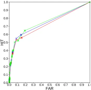
The ROC Curves relative to COSMO-LEPS and to the 5-RM EPS are shown for the event “average precipitation ex-ceeding 20 mm/24 h”, for the forecast ranges +66 h (Fig. 8) and +90 h (Fig. 9). The “cleps” curves (blue curves) are above the “epsrm” ones (red curves) for both forecast ranges. Considering the first cross from the top right in the diagrams,

(7)

532 C. Marsigli et al.: COSMO-LEPS verification

24 48 72 96 120 forecast range (h) -0.2 0 0.2 0.4 0.6

brier skill score

20mm

cleps epsrm

eps51

Fig. 8. Average values: ROC Curves for the precipitation threshold 20 mm/24 h and for the +66 h forecast range. The blue line is relative to cleps while the red line is relative to the epsrm.

24 48 72 96 120 forecast range (h) -0.2 0 0.2 0.4 0.6

brier skill score

20mm

cleps epsrm

eps51

Fig. 9. Average values: ROC Curves for the precipitation threshold 20 mm/24 h and for the +90 h forecast range. The blue line is relative to cleps while the red line is relative to epsrm.

it is evident that the two systems have comparable False Alarm Rate, but COSMO-LEPS obtains higher Hit Rate val-ues. This cross is correspondent to the probabilistic issue “at least one ensemble member is forecasting the event”, whose practical meaning can be understood referring to a alert situ-ation. If a user have a damage from the considered event, he can avoid the related loss by taking a preventive action. In

C. Marsigli et al.: COSMO–LEPS verification 7

24 48 72 96 120 forecast range (h) -0.2 0 0.2 0.4 0.6

brier skill score

20mm

cleps epsrm

eps51

Fig. 10. Brier Skill Score values for the precipitation threshold

20mm/24h. The blue line is relative to cleps, the red line is rela-tive to epsrm, the green line is for eps51. Maximum observed and forecast values over 1.5 x 1.5 degree boxes are compared.

curves) are above the “epsrm” ones (red curves) for both forecast ranges. Considering the first cross from the top right in the diagrams, it is evident that the two systems have com-parable False Alarm Rate, but COSMO–LEPS obtains higher Hit Rate values. This cross is correspondent to the proba-bilistic issue “at least one ensemble member is forecasting the event”, whose practical meaning can be understood re-ferring to a alert situation. If a user have a damage from the considered event, he can avoid the related loss by taking a preventive action. In order to decide if the action has to be taken, he uses the probabilistic system, but he has to decide on which probability threshold to rely. The first cross of the diagram corresponds to the hit rate and false alarm rate a user can have if he decide to take a protective action when at least one ensemble member forecasts the event, so he rely on a very low probability threshold. This situation is usually linked with cases in which the possible loss is very high (hu-man lives) with respect to the cost of the preventive action. Finally, it has to be reminded that the very first point of both curves, with co-ordinates (1,1), is just a theoretical limit to which the curves are extrapolated. Then, the first cross has to be considered the first significant point of the curves.

Averaging the precipitation over boxes of this size per-mits us to understand if the amount of precipitation over a vast region is correctly forecast, without giving information on precipitation peaks, which are very important for hydro– geological purposes. A high–resolution system can produce a significant improvement in the quantitative precipitation forecast if it is able to provide this kind of information. For this reason, a comparison in terms of precipitation maxima has been performed: the maximum forecast value falling in a box is compared with the maximum observed value in the same box. The boxes are of the same size, 1.5 x 1.5 degrees. The BSS values for cleps (Fig. 10, blue line) are clearly higher than those relative to both the epsrm and eps51 ones, indicating that COSMO–LEPS is better able to forecast the occurrence of high precipitation over an area. The system has a positive skill for all the forecast ranges. In terms of ROC area, Fig. 11, cleps still has the highest values, while

Fig. 11. ROC area for the precipitation threshold 20mm/24h. The

blue line is relative to cleps, the red line is relative to epsrm, the green line is relative to eps51. Maximum observed and forecast values over 1.5 x 1.5 degree boxes are compared.

0.0 0.1 0.2 0.3 0.4 0.5 0.6 0.7 0.8 0.9 1.0 FAR 0.0 0.1 0.2 0.3 0.4 0.5 0.6 0.7 0.8 0.9 1.0 HIT ROC curve - s066 t020 ROC curve - s066 t020

cleps max epsrm max

Fig. 12. Maximum values: ROC Curves for the precipitation

thresh-old 20mm/24h and for the +66h forecast range. The blue line is relative to cleps while the red line is relative to the epsrm.

the distance between eps51 and epsrm increases. In terms of both indices, the cleps performance worsens with increasing time range. At the +114 h forecast range, cleps has the same ROC area value as eps51, while in terms of BSS it still shows some improvement.

The ROC Curves relative to COSMO–LEPS and to the 5–RM EPS are shown for the event “maximum precipita-tion exceeding 20mm/24h”, for the forecast ranges +66 hours (Fig. 12) and +90 hours (Fig. 13). The “cleps” curves (blue curves) are well above the “epsrm” ones (red curves) for both forecast ranges. Considering the first cross from the top right in the diagrams (correspondent to the probabilistic issue “at least one ensemble member is forecasting the event”), the relationship between Hit Rate and False Alarm Rate of the two systems can be easily understood. At the +66 h (+90 h)

Fig. 10. Brier Skill Score values for the precipitation threshold 20 mm/24 h. The blue line is relative to cleps, the red line is rela-tive to epsrm, the green line is for eps51. Maximum observed and forecast values over 1.5×1.5◦ boxes are compared.

order to decide if the action has to be taken, he uses the prob-abilistic system, but he has to decide on which probability threshold to rely. The first cross of the diagram corresponds to the hit rate and false alarm rate a user can have if he de-cide to take a protective action when at least one ensemble member forecasts the event, so he relies on a very low prob-ability threshold. This situation is usually linked with cases in which the possible loss is very high (human lives) with re-spect to the cost of the preventive action. Finally, it has to be reminded that the very first point of both curves, with co-ordinates (1,1), is just a theoretical limit to which the curves are extrapolated. Then, the first cross has to be considered the first significant point of the curves.

Averaging the precipitation over boxes of this size per-mits us to understand if the amount of precipitation over a vast region is correctly forecast, without giving information on precipitation peaks, which are very important for hydro-geological purposes. A high-resolution system can produce a significant improvement in the quantitative precipitation forecast if it is able to provide this kind of information. For this reason, a comparison in terms of precipitation maxima has been performed: the maximum forecast value falling in a box is compared with the maximum observed value in the

same box. The boxes are of the same size, 1.5×1.5◦.

The BSS values for cleps (Fig. 10, blue line) are clearly higher than those relative to both the epsrm and eps51 ones, indicating that COSMO-LEPS is better able to forecast the occurrence of high precipitation over an area. The system has a positive skill for all the forecast ranges. In terms of ROC area, Fig. 11, cleps still has the highest values, while the distance between eps51 and epsrm increases. In terms of both indices, the cleps performance worsens with increasing time range. At the +114 h forecast range, cleps has the same ROC area value as eps51, while in terms of BSS it still shows some improvement.

The ROC Curves relative to COSMO-LEPS and to the 5-RM EPS are shown for the event “maximum precipitation ex-ceeding 20 mm/24 h”, for the forecast ranges +66 h (Fig. 12) and +90 h (Fig. 13). The “cleps” curves (blue curves) are