HAL Id: hal-00811524
https://hal.archives-ouvertes.fr/hal-00811524
Submitted on 10 Apr 2013
HAL is a multi-disciplinary open access
archive for the deposit and dissemination of sci-entific research documents, whether they are pub-lished or not. The documents may come from teaching and research institutions in France or abroad, or from public or private research centers.
L’archive ouverte pluridisciplinaire HAL, est destinée au dépôt et à la diffusion de documents scientifiques de niveau recherche, publiés ou non, émanant des établissements d’enseignement et de recherche français ou étrangers, des laboratoires publics ou privés.
Distribution Models Using Scene Identification from
Satellite Cloud Property Retrievals
Norman G. Loeb, Frédéric Parol, Jean-Claude Buriez, Claudine Vanbauce
To cite this version:
Norman G. Loeb, Frédéric Parol, Jean-Claude Buriez, Claudine Vanbauce. Top-of-Atmosphere
Albedo Estimation from Angular Distribution Models Using Scene Identification from Satellite Cloud Property Retrievals. American Meteorological Society, 2000, 13 (7), pp.1269-1285. �10.1175/1520-0442(2000)0132.0.CO;2�. �hal-00811524�
q2000 American Meteorological Society
Top-of-Atmosphere Albedo Estimation from Angular Distribution Models Using Scene
Identification from Satellite Cloud Property Retrievals
NORMANG. LOEB
Center for Atmospheric Sciences, Hampton University, Hampton, Virginia
FRE´ DE´RIC PAROL, JEAN-CLAUDEBURIEZ,AND CLAUDINEVANBAUCE
Laboratoire d’Optique Atmosphe´rique, Universite´ des Sciences et Technologies de Lille, Lille, France
(Manuscript received 5 March 1999, in final form 3 June 1999) ABSTRACT
The next generation of earth radiation budget satellite instruments will routinely merge estimates of global top-of-atmosphere radiative fluxes with cloud properties. This information will offer many new opportunities for validating radiative transfer models and cloud parameterizations in climate models. In this study, five months of Polarization and Directionality of the Earth’s Reflectances 670-nm radiance measurements are considered in order to examine how satellite cloud property retrievals can be used to define empirical angular distribution models (ADMs) for estimating top-of-atmosphere albedo. ADMs are defined for 19 scene types defined by satellite retrievals of cloud fraction and cloud optical depth. Two approaches are used to define the ADM scene types. The first assumes there are no biases in the retrieved cloud properties and defines ADMs for fixed discrete intervals of cloud fraction and cloud optical depth (fixed-t approach). The second approach involves the same cloud fraction intervals, but uses percentile intervals of cloud optical depth instead (percentile-t approach). Albedos generated using these methods are compared with albedos inferred directly from the mean observed reflectance field.
Albedos based on ADMs that assume cloud properties are unbiased (fixed-t approach) show a strong systematic dependence on viewing geometry. This dependence becomes more pronounced with increasing solar zenith angle, reachingø12% (relative) between near-nadir and oblique viewing zenith angles for solar zenith angles between 608 and 708. The cause for this bias is shown to be due to biases in the cloud optical depth retrievals. In contrast, albedos based on ADMs built using percentile intervals of cloud optical depth (percentile-t approach) show very little viewing zenith angle dependence and are in good agreement with albedos obtained by direct integration of the mean observed reflectance field (,1% relative error). When the ADMs are applied separately to populations consisting of only liquid water and ice clouds, significant biases in albedo with viewing geometry are observed (particularly at low sun elevations), highlighting the need to account for cloud phase both in cloud optical depth retrievals and in defining ADM scene types. ADM-derived monthly mean albedos determined for all 58 3 58 lat–long regions over ocean are in good agreement (regional rms relative errors ,2%) with those obtained by direct integration when ADM albedos inferred from specific angular bins are averaged together. Albedos inferred from near-nadir and oblique viewing zenith angles are the least accurate, with regional rms errors reaching ;5%–10% (relative). Compared to an earlier study involving Earth Radiation Budget Experiment ADMs, regional mean albedos based on the 19 scene types considered here show a factor-of-4 reduction in bias error and a factor-of-3 reduction in rms error.
1. Introduction
One of the major weaknesses in current climate mod-els is the manner in which clouds are represented (Cess et al. 1990). Current models have difficulty simulating even the gross zonal mean seasonal changes in cloud radiative forcing, and uncertainties on a regional scale are even larger (Hartmann et al. 1986; Kiehl et al. 1994;
Corresponding author address: Dr. Norman G. Loeb, Mail Stop
420, NASA Langley Research Center, Hampton, VA 23681-0001. E-mail: [email protected]
Chen and Roeckner 1996). Since clouds have a domi-nant influence on the geographic and temporal distri-bution of the earth radiation budget, global observations of top-of-atmosphere fluxes coincident with cloud prop-erties are needed to provide the information necessary to improve climate models. The Earth Radiation Budget Experiment (ERBE) (Barkstrom 1984) and the Scanner for Radiation Budget (Kandel et al. 1998) provided the most accurate top-of-atmosphere radiation budget mea-surements to date but did not provide details on the physical cloud properties. The International Satellite Cloud Climatology Project (ISCCP) (Rossow and Schif-fer 1991) and First ISCCP Regional Experiment (Cox
et al. 1987) provided valuable new datasets of cloud properties over different temporal and spatial scales but did not provide routine top-of-atmosphere radiation budget measurements. The next generation of satellite instruments such as Clouds and the Earth’s Radiant En-ergy System (CERES), Polarization and Directionality of the Earth’s Reflectances (POLDER), Multi-angle Im-aging Spectroradiometer, and Geostationary Earth Ra-diation Budget will routinely merge top-of-atmosphere radiative fluxes with cloud properties, thereby providing comprehensive global datasets for climate model stud-ies. Improved estimates of albedo, together with coin-cident cloud retrievals, will provide critical information needed to validate climate models and improve cloud parameterizations.
One of the largest sources of uncertainty in estimating planetary radiation budget from narrow field-of-view satellite instruments is the conversion of measured ra-diances to fluxes (Wielicki et al. 1995). The problem dates back to some of the earliest satellite measurements (House et al. 1986) and continues to be a major area of concern. Because satellite radiometers can only instan-taneously measure radiances in a limited number of viewing directions—while albedo or flux requires ra-diances from all angles—assumptions are needed to ac-count for the anisotropy (or angular variation) in the radiance field. ERBE used a set of 12 angular distri-bution models (ADMs) to convert the ERBE measured radiances to top-of-atmosphere (TOA) fluxes (Smith et al. 1986; Suttles et al. 1988). The ERBE ADMs were constructed using Nimbus-7 earth radiation budget (ERB) scanner data and were applied to ERBE radiance measurements on NOAA-9, -10, and the Earth Radiation Budget Satellite (ERBS) using scene identification based on the maximum likelihood estimation method (Wielicki and Green 1989). To construct the ERBE ADMs, the sorting into angular bins (SAB) method was used (Tay-lor and Stowe 1984). Postflight analyses have revealed some problems with ERBE radiative fluxes. Payette (1989) and Suttles et al. (1992) have shown that esti-mated shortwave fluxes increase systematically with viewing zenith angle and estimated longwave fluxes de-crease with viewing zenith angle. The cause for such biases is believed to be due either to the methodology used in deriving ERBE ADMs (Suttles et al. 1992; Green and Hinton 1996) and/or to errors in scene iden-tification (Ye and Coakley 1996; Smith and Manalo-Smith 1995).
Large errors in ADM derived albedos can also occur if the scene category an ADM is defined for is too general or encompasses too wide a range of surface types (i.e., if the ADM variance is large) (Green and Hinton 1996). One method of reducing such errors is to increase the number of scene types or classes the ADMs are defined for (Wielicki et al. 1996). Since the anisotropy of earth scenes depends on their physical and optical properties (e.g., cloud fraction, cloud optical depth, etc.), a logical approach is to define ADM scene
types from satellite-derived cloud retrievals. However, as pointed out by Loeb and Davies (1996) and Loeb and Coakley (1998), satellite retrievals (particularly cloud optical depths based on 1D theory) can suffer from large systematic biases that depend on viewing geometry. Such biases are shown here to be of major importance for TOA albedo estimation based on the ADM approach.
In the following, three months of POLDER mea-surements are used to construct ADMs at a wavelength of 670 nm for scene types defined by satellite retrievals of cloud fraction and cloud optical depth. Two ap-proaches are considered in building the ADMs. The first assumes there are no biases in the cloud property re-trievals and defines ADMs for 19 scene types stratified by fixed discrete intervals of cloud fraction and cloud optical depth. The second, more general, approach uses the same cloud fraction intervals but allows for potential biases in the cloud optical depth retrievals by defining ADM scene types for percentile intervals of cloud op-tical depth in each angular bin rather than fixed intervals of cloud optical depth. Albedos estimated from the two sets of ADMs are compared with mean albedos inferred by direct integration of mean reflectances using two independent months of POLDER data.
2. Observations
The POLDER instrument flew on the Advanced Earth Observation Satellite (ADEOS) between August 1996 and June 1997. POLDER is a camera composed of a two-dimensional charged coupled device detector array, wide field-of-view telecentric optics, and a rotating wheel carrying spectral and polarized filters. POLDER is in a sun-synchronous orbit with an equatorial crossing time of 1030 LT, has a swath width of approximately 2200 km, and a pixel size of about 6 3 7 km2at nadir.
As the satellite moves over a region, up to 14 different images are acquired in each spectral band from various geometric configurations. Figure 1 provides an example of the angular sampling typical of POLDER. It shows the viewing zenith and relative azimuth angle coverage within the region defined by a latitude of 08 6 0.58 and a longitude of 08 6 0.58 for seven days in November 1996. Each day, the region is sampled from a different set of viewing directions, so that full azimuth and view-ing zenith (up toø608) angle coverage is obtained by compositing measurements over time. POLDER spec-tral bands are shown in Table 1. Note that only channels with the wider dynamic range are used in the POLDER level-2 ERB and clouds product (Buriez et al. 1997) considered in this study. POLDER calibration uncer-tainty is estimated to be ,3%–4% (Hagolle et al. 1999). A more detailed description of the POLDER instrument is provided by Deschamps et al. (1994).
In this study, five months (November 1996; January, April, May, and June 1997) of POLDER level-2 ERB and clouds product data (Buriez et al. 1997) over ocean
FIG. 1. Angular sampling typical of POLDER. Each set of points (i.e., on a given day) corresponds to viewing zenith and azimuthal angles for near-simultaneous measurements over a region defined by a lat of 08 6 0.58 and a long of 08 6 0.58 (Nov 1996). Each day, the region is sampled from a different set of viewing directions, so that full azimuth and viewing zenith (up toø608) angle coverage is obtained by compositing measurements over time.
TABLE1. Characteristics of the spectral bands of the POLDER instrument. Dynamic range is the range in equivalent reflectance [5p *I/F; I 5 radiance (W m22sr21mm21); F 5 solar irradiance (W
m22mm21)] that POLDER channels are sensitive to.
Central wavelength (nm) Bandwidth (nm) Polarization Dynamic range 443 443 490 565 670 763 765 865 910 20 20 20 20 20 10 40 40 20 No Yes No No Yes No No Yes No 0–0.22 0–1.10 0–0.17 0–0.11 0–1.10 0–1.10 0–1.10 0–1.10 0–1.10
between 608S and 608N are considered. Briefly, the lev-el-2 ERB and clouds product provides cloud properties (cloud fraction, cloud phase, cloud optical depth, ap-parent pressure, etc.) and radiances in all viewing di-rections overø56 3 56 km2‘‘super-pixel’’ regions (ø9
3 9 full-resolution 6 3 7 km2POLDER pixels). Cloud
fractions are determined by applying a cloud detection algorithm to each full-resolution POLDER pixel and direction. The cloud detection scheme consists of a se-quence of threshold tests on a pixel’s apparent pressure, reflectance (865 nm over ocean, 443 nm over land), 443-and nm polarized radiance, 443-and the ratio of 865-and 443-nm channel reflectances (Parol et al. 1999). Cloud phase is determined using polarized reflectance at 865 nm (Parol et al. 1999). The algorithm takes ad-vantage of the differences in polarized reflectance be-tween liquid water and ice clouds in different scattering angle ranges. For example, (i) polarized reflectance from liquid water clouds increases with scattering angle (Q)
TABLE2. Angular bin definitions (8). Solar zenith angle (uo) Viewing zenith angle (u) Relative azimuth (f ) 0–10 10–20 20–30 30–40 40–50 50–60 60–70 70–80 80–90 0–10 10–20 20–30 30–40 40–50 50–60 0–10 10–30 30–50 50–70 70–90 90–110 110–130 130–150 150–170 170–180 for 608 , Q , 1408, while the opposite is true for ice
clouds; (ii) for 1358 , Q , 1458, the polarized reflec-tance from liquid water clouds shows a distinct peak (primary rainbow) that is not apparent for ice clouds; and (iii) for 1408 , Q , 1808, the magnitude of polarized reflectance is typically larger for liquid water clouds than for ice clouds. Cloud optical depth is estimated for each full-resolution POLDER pixel and direction flagged as cloud-contaminated using a look-up table approach based on plane-parallel theory. In the current version of the POLDER level-2 product, the cloud layer is assumed to be composed of liquid water droplets with an effective radius of 10 mm and an effective variance of 0.15 (Han-sen and Travis 1974). Future versions of the POLDER algorithm will improve the treatment of ice clouds by using more realistic phase functions based on represen-tative ice particle shapes (Parol et al. 1999). The full-resolution cloud optical depth retrievals in each viewing direction are converted into equivalent 1D spherical al-bedos, which are averaged spatially over the super-pixel. An energy-equivalent cloud optical depth in each viewing direction is inferred from the super-pixel cloud spherical albedos following the approach of Rossow et al. (1996) (Parol et al. 1999).
3. Methodology
a. Albedo estimation from POLDER reflectances The fact that POLDER measurements are restricted to viewing zenith angles less thanø608 requires a slight-ly different approach for defining ADMs than the con-ventional approach of Taylor and Stowe (1984). Here, an empirical ‘‘partial’’ ADM (Rp,j) is first defined for a given scene type from the following:
r (u , u, f )j o
R (u , u, f ) 5p, j o , (1)
A (u )p, j o
where rjand Ap,jare the mean reflectance and partial albedo for scene type ‘‘j’’ given by
pI (u , u, f)j o r (u , u, f ) 5j o
7
8
(2) cos(u )Eo o 2p 1 A (u ) 5p, j oE E
r m dm dfj (3) 0 mm Ij instantaneous radiance (W m22 sr21mm21),Eo solar irradiance (W m22mm21) corrected for Earth–
Sun distance,
u viewing zenith angle,
uo solar zenith angle,
f azimuth angle relative to the solar plane defined between 08 and 1808 (f 5 08 corresponds to for-ward scattering),
m cosine of viewing zenith angle.
In Eq. (3), mm 5 cosum, where um is the maximum
viewing zenith angle where observations are consis-tently obtained. A value of 558 for umis used since this corresponds to the midpoint of the most oblique angular bin. Bin mean reflectances are determined over 108 solar and viewing zenith angle bins, and over relative azimuth angle bins of width 208 between f 5 108 and f 5 1708, and 108 elsewhere (see Table 2). The integral in Eq. (3) is evaluated using Gaussian quadrature by in-terpolating rjto Gauss–Legendre abscissas (200 quad-rature points are considered).
An instantaneous reflectance measurement [rj(uo, u,
f )] is converted to a partial albedo [Aˆp(uo, u, f )] by first identifying the appropriate ADM scene type and applying the partial ADM as follows:
r (u , u, f )j o ˆ
A (u , u, f ) 5p o . (4)
R (u , u, f )p, j o
Next, the albedo over the entire upward hemisphere or ‘‘full’’ albedo [Aˆ (uo, u, f )] is estimated from Aˆp(uo,
u, f ) using a theoretical conversion. Figures 2a–c show
theoretical full against partial albedos for three solar zenith angles at a wavelength of 670 nm. The curves were inferred from three sources: (i) clear-sky values were based on MODTRAN (Kneizys et al. 1996) cal-culations modified to account for ocean bidirectional reflectance according to the Cox and Munk (1954) for-mulation; (ii) 1D liquid and ice cloud [using the mea-sured ice phase function of Sassen and Liou (1979)] values are based on DISORT (Stamnes et al. 1988) cal-culations for cloud optical depths ranging between 0.5 and 200; and (iii) 3D cloud values are based on Monte Carlo simulations (no atmospheric scattering) for 16 broken and overcast stochastic cloud fields with bumpy tops (Va´rnai 1996; Loeb et al. 1998). Cloud fractions ranged from 0.25 to 1.0, and averaged cloud optical depths were between 5 and 160 (see Table 3). As shown in Figs. 2a–c, a very simple relationship between partial and full albedo is obtained, even for horizontally in-homogeneous cloud fields. To infer Aˆ from Aˆp, fits to the curves in Figs. 2a–c are applied. These have the form: 3 i ˆ ˆ A(u , u, f ) 5o
O
a (u )A (u , u, f ),i o p o (5) i50FIG. 2. Full and partial albedos (%) from theory for clear and cloudy conditions at (a) uo5 258; (b) uo5 458, and (c) uo5 658. Curve is
a third-order polynomial fit to all points.
TABLE3. Cloud fractions and cloud optical depths of cloud fields used in Monte Carlo model simulations considered in Figs. 2a–c.
Cloud
fraction Cloud optical depth
0.25 0.50 0.75 1.00 20 10 6.7 5 40 20 13.3 10 80 40 26.7 20 160 80 53.3 40
where ai’s are coefficients of a third-order polynomial. For the cloud fields considered in Figs. 2a–c, root-mean-square (rms) errors based on these fits are less than
;1%.
b. ADM scene types
The purpose of defining ADMs by scene type is to better account for the variability in the anisotropy of earth scenes. Since earth scenes have distinct anisotropic characteristics that depend on their physical and optical properties (e.g., thin vs thick clouds, cloud-free, broken, overcast, etc.), it seems reasonable to define ADM scene types from scene parameters that have the greatest in-fluence on anisotropy. To illustrate, Figs. 3a–b show ADMs constructed from POLDER measurements for overcast scenes with cloud optical depth (t ) , 2.5 (Fig. 3a) and t 5 18–40 (Fig. 3b). The ADMs were deter-mined by replacing the denominator in Eq. (1) with mean albedos obtained by averaging instantaneous full
albedos inferred from Eqs. (4)–(5). Differences between the two ADMs are as large as a factor of 2 close to nadir but decrease with increasing viewing zenith angle. In order to define ADM scene types based on cloud optical properties, an obvious approach is to use satellite retrievals of these parameters (e.g., cloud fraction, cloud optical depth, etc.). However, since ADMs are con-structed by compositing radiances from many scenes measured in different satellite viewing geometries, this approach assumes that scene identification is consistent with angle. That is, it assumes that a given scene type (e.g., defined for a given cloud property interval) iden-tified from one satellite viewing geometry can be con-sistently identified from all other directions. Since sat-ellite-based retrievals often rely on simplified radiative transfer models (e.g., plane-parallel theory) that use ide-alized cloud microphysics (e.g., particle shape and phase), this poses a potential problem. Loeb and Davies (1996) and Loeb and Coakley (1998) showed that cloud optical depth retrievals based on 1D theory show a sys-tematic dependence on solar zenith and viewing zenith angle, even for overcast marine stratiform clouds—ar-guably the closest to plane-parallel in nature. Mish-chenko et al. (1996) demonstrated theoretically how in-correct assumptions on cloud particle shape and phase can result in large angle-dependent errors in retrieved cloud optical depths. Figures 4a–b show mean cloud optical depth retrievals against solar zenith and viewing zenith angle (azimuthally averaged) from two months (January and May 1997) of POLDER measurements for all overcast clouds (Fig. 4a) and for overcast clouds composed only of liquid water droplets as determined by the POLDER cloud phase algorithm (Fig. 4b). As shown, a systematic dependence in retrieved cloud op-tical depth on viewing zenith angle is observed in both cases for solar zenith angles .508, in a manner consis-tent with the earlier studies.
The question arises as to whether such biases in cloud optical depth retrievals introduce similar biases in ADM derived albedos. To answer this question, two approach-es (dapproach-escribed below) are considered in constructing par-tial ADMs for 19 scene classes based on POLDER an-gle-dependent cloud fraction and cloud optical depth retrievals. Both sets of ADMs assume the same six cloud fraction intervals (Table 4) but employ a different cloud optical depth stratification. To construct the partial ADMs, three months of POLDER observations (No-vember 1996, April and June 1997) are considered.
FIG. 3. Overcast ADMs [R(uo, u, f )] from POLDER 670-nm reflectance measurements for uo5 608–708. (a) t , 2.5
FIG. 4. Mean retrieved cloud optical depth inferred from two months (Jan and May 1997) of POLDER measurements for overcast scenes against solar zenith and viewing zenith angle (azimuthally averaged) for (a) all clouds and (b) clouds composed only of liquid water droplets as determined by the POLDER cloud phase algorithm.
TABLE4. Cloud fraction and cloud optical depth intervals defining ADM scene types.
Cloud fraction interval (%) Cloud optical depth fixed interval Cloud optical depth percentile interval Total 0–1 All 0–100 1 1–25 0–1.5 .1.5 0–50 50–100 2 25–50 0–1.5 .1.5 0–50 50–100 2 50–75 0–1 1–2.5 .2.5 0.0–33.3 33.3–66.6 66.6–100 3 75–99 0–1 1–2 2–3 3–5 .5 0.0–20 20–40 40–60 60–80 80–100 5 99–100 0–2.5 2.5–6 6–10 10–18 18–40 .40 0–5 5–25 25–50 50–75 75–95 95–100 6
1) PARTIALADMS BASED ON FIXED ABSOLUTE INTERVALS OF CLOUD OPTICAL DEPTH
Assuming cloud optical depth retrievals are perfect in all viewing geometries, each of the six cloud fraction intervals in Table 4 can be stratified into fixed discrete intervals of cloud optical depth. Note that the number of cloud optical depth intervals in Table 4 increases with cloud fraction. The reason is because cloud optical depth distributions have a tendency to broaden with increasing cloud cover, so that more intervals are needed to cover the full range of cloud optical depth at larger cloud fractions. A similar broadening in cloud optical depth distributions with cloud cover was also observed by Barker et al. (1996). For each cloud fraction–cloud op-tical depth interval, a partial ADM is determined by compositing the POLDER 670-nm reflectances in each angular bin and calculating the partial ADM using the approach described in section 3a. In order to reduce sampling bias errors due to temporal and spatial
auto-correlation between pixel measurements, the month mean reflectance values in each angular bin are calcu-lated from daily mean reflectances, which are assumed independent. Hereafter, this approach is referred to as the fixed-t approach.
2) PARTIALADMS BASED ON FIXED PERCENTILE INTERVALS OF CLOUD OPTICAL DEPTH
An alternate, more general, approach is to define ADM scene types using percentile intervals of cloud optical depth rather than fixed discrete intervals of cloud optical depth [as in section 3b(1)]. The aim is to define ADM scene types that can be identified consistently from all angles, regardless of whether cloud optical depth retrievals show biases with viewing geometry. As an example, an ADM scene type for the thinnest 5% of all overcast scenes can be defined by compositing scenes in each angular bin with a retrieved cloud optical depth that lies below a predetermined (angle-dependent) threshold that corresponds to the 5th percentile of cloud optical depth. Predetermined cloud optical depth thresh-olds (corresponding to a given cloud optical depth per-centile) are inferred from frequency distributions of cloud optical depth from a large ensemble of measure-ments. Separate cloud optical depth thresholds are de-fined for each angular bin. Consequently, scenes cor-responding to a given cloud optical depth percentile interval range (e.g., thinnest 5% of the population) are grouped consistently in all angles. It is worth noting that while the percentile-t approach attempts to reduce the effect of scene identification errors on albedo, it does
not reduce biases in the cloud property retrievals them-selves. Such a correction would require a reassessment of the cloud retrieval scheme. Hereafter, this approach is referred to as the percentile-t approach.
Scene types for partial ADMs based on the percen-tile-t approach are provided in Table 4. Note that the same cloud fraction intervals used in defining fixed-t ADMs are also used for the percentile-t ADMs. c. Mean ADM albedo validation using direct
integration method
ADMs provide instantaneous fluxes or albedos at the time of the satellite overpass. Instantaneous fluxes are needed together with narrowband measurements from geostationary satellites to estimate diurnal means, which are used to estimate monthly mean fluxes (Young et al. 1998). One method of validating ADMs is to separate ADM errors from diurnal modeling errors by ignoring diurnal effects. ADM albedo averages determined from a large ensemble of measurements (e.g., one or several months) are compared with mean albedos determined by direct integration of the mean reflectances. The mean ADM albedos are inferred from instantaneous ADM albedo estimates and are stratified by solar zenith, view-ing zenith, and relative azimuth angle bins. A direct integration mean albedo (for a given solar zenith angle bin) is computed by compositing all reflectances (re-gardless of scene type) into angular bins and directly integrating the mean reflectances [r (uo, u, f )]. Since the same data are used in both cases, and since no diurnal effects are involved, differences between the ADM and direct integration mean albedos are due to ADM errors. Unfortunately, since viewing zenith angles .608 are not consistently available from POLDER, it is only pos-sible to use direct integration to determine mean partial albedos (AD(uo)). Since AD(uo) is determined using all
p p
scenes (so that no scene identification errors are intro-duced), comparison betweenAD(uo) and the mean
par-p
tial albedo based on partial ADMs [A (u , u, f )ˆp o ] pro-vides an estimate of the error inA (u , u, f )ˆp o . To esti-mate the uncertainty in the full ADM albedo [A(u , u, f )ˆ o ], an estimate of the full direct integration albedo [AD(uo)] is needed. We estimate AD(uo) using the assumption that the relative error in the full angle-average ADM albedo is the same as that for the partial angle-average ADM albedo. That is, we assume
D D ˆ ˆ A (u ) 2 A (u ) A(u ) 2 A (u )o o p o p o 5 , (6) D D A (u )o A (u )p o
whereA (uˆp o) andA(u )ˆ o are the partial and full angle-average ADM albedos obtained by averaging mean al-bedos from all available viewing zenith and relative azimuth angular bins (Table 2). An estimate of AD(uo) is obtained by rearranging the terms in Eq. (6) as fol-lows: ˆ A(u )o D D A (u ) 5 A (u )o p o ˆ . (7) A (u )p o
The error in A(u , u, f )ˆ o is thus determined by com-parison with AD(uo), assuming that AD(uo) represents the ‘‘true’’ mean albedo. Since AD(uo) is based on an assumption [Eq. (6)] that depends on a ratio between ADM derived albedos, there is some uncertainty in AD(uo). Sensitivity in AD(uo) to the ADM albedo ratio in Eq. (7) is estimated to be ,0.25% (relative) based on comparisons between percentile-t , fixed-t , and Lam-bertian (i.e., no angular correction) ADMs. If the direct integration technique is applied using a subset of scenes (e.g., specific cloud fraction range), errors in scene iden-tification can also occur since the true scene identifi-cation is not available.
4. Results
In some applications, such as the use of TOA albedos in conjunction with surface measurements, it is not al-ways feasible to collect albedos for all scene types in all satellite-viewing geometries. Instead, it may be nec-essary to restrict the sampling to a small range of angles (e.g., near-nadir views). Therefore, a powerful check on the quality of the ADMs is to statistically test whether they provide consistent albedo estimates in all viewing geometries. Here, this criterion is used extensively to evaluate the performance of the fixed-t and percentile-t approaches.
In the following, mean albedos inferred using fixed-t and percentile-t ADMs are compared with albedos ob-tained by direct integration of mean reflectances. As noted earlier, the ADMs were constructed from three months of POLDER measurements (November 1996, April and June 1997). The ADMs are now applied to produce albedo estimates from two independent months (January and May 1997).
a. Albedo and cloud property retrieval viewing zenith angle dependence
To compare albedos obtained from fixed-t and per-centile-t ADMs, it is useful to first restrict the analysis to overcast (cloud fraction . 0.99) scenes. Figures 5a–f show overcast mean albedos and mean cloud optical depth retrievals against viewing zenith angle for solar zenith angles between 208 and 308 (Figs. 5a,b), 408 and 508 (Figs. 5c,d), and 608 and 708 (Figs. 5e,f). Each mean ADM derived albedo in a given viewing zenith angle bin was determined by averaging mean albedos from 10 relative azimuth bins (Table 2), so that each relative azimuth bin contributes an equal weight to the overall mean.
As shown in Figs. 5a, 5c, and 5e, albedos obtained using the fixed-t ADMs show a large dependence on viewing zenith angle. The viewing zenith angle depen-dence closely follows that in the mean cloud optical
FIG. 5. (left) Mean albedos and (right) mean retrieved cloud optical depths against viewing zenith angle for uobetween (a), (b) 208 and 308; (c), (d) 408 and 508; and (e), (f ) 608 and 708.
depth retrievals (Figs. 5b, 5d, and 5f) and becomes more pronounced with increasing solar zenith angle—fixed-t albedos decrease by as much asø12% between near-nadir and oblique viewing zenith angles for uo5 608–
708. In contrast, albedos based on the percentile-t ADMs show very little dependence on viewing zenith angle and are in good agreement with albedos obtained by direct integration.
Figures 6a–f show similar results to those in Figs. 5a–f, but for all scenes. Also, mean cloud fraction re-trievals are provided in Figs. 6b, 6d, and 6f instead of mean cloud optical depth. As shown, the viewing zenith
angle dependence in mean cloud fraction retrievals is much smaller than that in mean cloud optical depth (Figs. 5b, 5d, and 5f). Because fixed absolute intervals of cloud fraction were used to define the ADM scene types, any viewing zenith angle dependence in albedo from the percentile-t ADMs closely follows that in mean cloud fraction. In contrast, mean albedos based on the fixed-t approach are influenced by viewing zenith angle biases in both cloud fraction and cloud optical depth (the latter being more pronounced in this case).
Since climate research requires an understanding of how albedo responds to changes in cloud properties,
FIG. 6. (left) Mean albedos and (right) mean cloud fractions against viewing zenith angle for uo
between (a), (b) 208 and 308; (c), (d) 408 and 508; and (e), (f ) 608 and 708.
satellite-based estimates of these parameters need to be consistently identified under a wide range of cloud and viewing conditions. Figures 7a–i compare the relation-ship between albedo and cloud fraction for different viewing zenith and solar zenith angle bins for the fixed-t and percentile-t approaches. Figures 7a–c show the di-rect integration albedo, which is assumed to represent the true albedo (i.e., errors in cloud fraction are assumed to be negligible), while the remaining curves provide relative errors in ADM derived albedos for different solar zenith angle ranges (relative error 5 [(Ae2 A)/A]
3 100%, where Ae is the estimate and A is ‘‘truth’’). For the fixed-t approach, relative errors in albedo are generally ,2% for uo5 208–308 (Fig. 7d) and show a
weak dependence on cloud fraction. As solar zenith an-gle increases, the relative errors increase and show a stronger dependence on cloud fraction. For uo5 408–
508 (Fig. 7e), relative errors are generally negative at all viewing zenith angles for cloud fractions ,0.25 (reaching 26%) and positive for cloud fractions .0.50 (reaching 5%). At lower sun (uo 5 608–708), relative
FIG. 7. (a)–(c) Direct integration mean albedo against cloud fraction; relative error in (d)–(f ) fixed-t and (g)–(i) percentile-t ADM albedos against cloud fraction for various solar zenith and viewing zenith angle ranges.
fractions between 75% and 99%) and show a larger dependence on viewing zenith angle (Fig. 7f). Results are much more encouraging for the percentile-t ap-proach—relative errors are generally ,2% for all solar zenith angles observed by POLDER over the full cloud fraction range.
b. Albedo errors due to neglect of cloud phase Given that the ADMs in this study are defined only in terms of cloud fraction and cloud optical depth, the question arises as to whether other cloud parameters are likely to have a significant influence on cloud anisotropy and albedo. Based on several studies (Minnis et al. 1993;
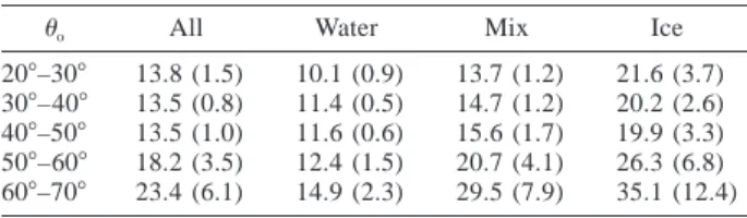
Mishchenko et al. 1996; Descloitres et al. 1998), an obvious candidate is cloud phase. To examine the im-portance of cloud phase on albedo estimation, the ADMs defined in section 3 were applied separately to overcast scenes for all conditions, clouds composed only of liquid water droplets, clouds containing both liquid droplets and ice particles (‘‘mixed-phase’’ clouds), and clouds containing only ice particles. Figures 8a–p show the viewing zenith angle and relative azimuth angle depen-dence in cloud optical depth and albedo for each of these cases in two solar zenith angle bins (uo5 308–408 and uo5 608–708) for the percentile-t approach, and Tables 5–7 provide the overall means and standard deviations determined from individual angular bin means (i.e., 6
V OL UME 13 JOURNAL OF CLIMATE
FIG. 8. (a)–(p) Mean cloud optical depth and mean albedo (%) based on the percentile-t ADMs for overcast scenes consisting of all cloud conditions, liquid, mixed-phase, and ice-phase, for uo5 308–408 and uo5 608–708. The bidirectional plots use the same angle convention as that shown in Figs. 3a,b.
TABLE5. Cloud optical depth mean and std dev (in parentheses) inferred from means in individual viewing zenith and relative azimuth angle bins.
uo All Water Mix Ice
208–308 308–408 408–508 508–608 608–708 13.8 (1.5) 13.5 (0.8) 13.5 (1.0) 18.2 (3.5) 23.4 (6.1) 10.1 (0.9) 11.4 (0.5) 11.6 (0.6) 12.4 (1.5) 14.9 (2.3) 13.7 (1.2) 14.7 (1.2) 15.6 (1.7) 20.7 (4.1) 29.5 (7.9) 21.6 (3.7) 20.2 (2.6) 19.9 (3.3) 26.3 (6.8) 35.1 (12.4)
TABLE6. Percentile-t albedo mean and std dev (in parentheses) inferred from means in individual viewing zenith and relative azimuth angle bins.
uo All Water Mix Ice
208–308 308–408 408–508 508–608 608–708 0.451 (0.008) 0.489 (0.006) 0.517 (0.003) 0.560 (0.004) 0.614 (0.006) 0.426 (0.006) 0.478 (0.008) 0.507 (0.006) 0.540 (0.007) 0.591 (0.011) 0.446 (0.014) 0.490 (0.011) 0.521 (0.016) 0.547 (0.009) 0.601 (0.011) 0.514 (0.012) 0.538 (0.011) 0.560 (0.011) 0.600 (0.017) 0.666 (0.019) viewing zenith angle 3 10 relative azimuth angle bins).
For uo5 308–408, the most persistent feature in both
the cloud optical depth and albedo results is the peak between u 5 308 and u 5 408 in the forward scattering direction. This feature likely corresponds to sun glint, perhaps due to ambiguities in ocean surface correction in the presence of thin clouds, or possibly due to clear-sky breaks in the POLDER full-resolution pixels. At other angles, the percentile-t albedo estimates appear reasonable (the overall albedo standard deviation in Ta-ble 6 is &0.01). There does appear to be a slight de-pendence on relative azimuth angle; however, slightly lower albedos occur in the backscattering direction, a trend that is more pronounced (relative difference be-tween forward and backscattering albedos of ø5%) when only ice clouds are considered (Fig. 8m).
For uo 5 608–708, the influence of cloud phase is
much stronger. In all cases, a significant decrease in mean cloud optical depth with viewing zenith angle oc-curs in the forward scattering direction. For liquid water clouds, this decrease is more than a factor of 2 (from 17 close to nadir to 8 between u 5 508 and u 5 608). In the backscattering direction, optical depths show a much smaller change (ø10%). These results are con-sistent with those reported by Loeb and Coakley (1998). In that study, cloud optical depths for moderate solar zenith angles decreased from 14 to 8 in the forward scattering direction, while there was very little variation with viewing zenith angle in the backscattering direc-tion. Loeb et al. (1998) were able to reproduce this behavior in Monte Carlo simulations when variations in cloud-top structure (‘‘cloud bumps’’) were included.
For mixed-phase and ice clouds, a sharp decrease in cloud optical depth with viewing zenith angle occurs in the forward and backscattering directions. Mean cloud optical depths are 3 times larger than those from liquid water clouds at nadir and at relative azimuth angles
betweenø708 and 1108, whereas optical depths in the forward scattering direction (f 5 08–308) are similar for liquid water and ice clouds. These findings are qual-itatively consistent with simulations by Mishchenko et al. (1996), who showed that reflectances from liquid water clouds tend to be lower than those from ice clouds close to nadir and at side-scattering angles, while the opposite is true at oblique viewing zenith angles in the forward and backscattering directions. Such differences would cause retrieved cloud optical depths (i.e., using a liquid water cloud model) to show a pattern similar to that in Fig. 8p.
For uo5 608–708, albedos inferred from the
percen-tile-t ADMs show little dependence on viewing ge-ometry when applied to all overcast clouds (Fig. 8d). In contrast, significant biases occur when albedos are stratified by cloud phase. Interestingly, while the overall bidirectional patterns in mean albedo for liquid water (Fig. 8h) and ice clouds (Fig. 8e) are qualitatively sim-ilar, the relative position of albedo minima and maxima for these two cases is interchanged. This suggests that significant cancellation of error must occur when all cloud types are combined (Fig. 8d). Standard deviations in albedo are largest for ice clouds (;0.019) and small-est when the ADMs are applied to all clouds (0.006; Table 6). By comparison, when the fixed-t ADMs are used (Table 7), standard deviations areø0.044 for ice clouds and ø0.032 for all clouds.
It is clear from these results that there is a need to account for cloud phase both in cloud optical depth retrievals and in defining ADM scene types. Stratifying by cloud phase and defining ADMs using the percen-tile-t approach appear to be the most promising means of reducing albedo errors.
c. Regional monthly mean albedos
Monthly mean albedos were determined for all 58 3 58 lat–long regions over ocean between 608S and 608N for different solar zenith and viewing zenith angle rang-es. The regional monthly albedos are not true monthly averages because no diurnal effects have been consid-ered. Instead, the averages were determined from all monthly samples falling in each angular bin at the time of observation. For each region, ADM derived albedos were compared with albedos determined by direct in-tegration. Figures 9a–d provide bias and rms errors for fixed-t and percentile-t ADMs. For comparison, Figs.
TABLE7. Fixed-t albedo mean and std dev (in parentheses) inferred from means in individual viewing zenith and relative azimuth angle bins.
uo All Water Mix Ice
208–308 308–408 408–508 508–608 608–708 0.449 (0.018) 0.489 (0.011) 0.518 (0.013) 0.563 (0.026) 0.615 (0.032) 0.424 (0.018) 0.478 (0.011) 0.509 (0.012) 0.543 (0.023) 0.593 (0.025) 0.444 (0.018) 0.490 (0.015) 0.522 (0.026) 0.549 (0.029) 0.602 (0.036) 0.513 (0.021) 0.538 (0.015) 0.562 (0.020) 0.602 (0.030) 0.667 (0.044)
FIG. 9. Bias and rms errors in monthly mean albedos determined for all 58 3 58 lat–long regions over ocean between 608S and 608N for different solar zenith and viewing zenith angle ranges. (a)–(d) provide bias and rms differences for fixed-t and percentile-t ADMs. For comparison, (e), (f ) show results obtained when no angular correction (i.e., ‘‘Lambertian’’) is assumed.
9e–f show results when no angular correction (i.e., ‘‘Lambertian’’) is used. If no angular correction is used, bias and rms errors increase sharply with solar zenith angle for oblique and near-nadir viewing zenith angles, reaching ø0.1 for uo 5 608–708. In contrast, when monthly mean albedos are inferred by averaging albedos from all viewing zenith angles, errors are drastically reduced (&0.005), even for the Lambertian case. Albedo biases for the fixed-t approach are most pronounced for
uo5 608–708, reachingø0.02, while bias errors for the percentile-t approach generally remain ,0.01 at all an-gles. Rms errors show a clear trend with both solar and viewing zenith angle, with larger values close to nadir and oblique viewing zenith angles.
Suttles et al. (1992) compared global ERBE ADM albedos over 500 km 3 500 km regions with albedos inferred by direct integration (which they refer to as the SAB method). ERBE ADM albedos showed a bias of 1.2% (relative) and a regional rms difference of 6% (relative). The corresponding values from the present study based on the percentile-t approach are 0.3% and 1.9%, a reduction by a factor 4 in bias error and a factor of 3 in rms error. The likely reason for this reduction in error is the number of scene types considered: ERBE considered only four classes of cloud cover (clear, partly cloudy, mostly cloudy, and overcast) compared to 19 in the present study. The larger number of scene types improves albedo estimates by increasing ADM sensi-tivity to scene parameters that have the greatest influ-ence on anisotropy (cf. Figs. 3a,b). Interestingly, the reduction in error based on the current set of 19 ADMs (compared to ERBE) is consistent with the expected reduction in error for CERES albedos based on a new set of CERES ADMs defined for a larger set of scene types (Wielicki et al. 1995). Further improvements in regional mean albedo accuracy are expected by further stratifying scene types by cloud phase (section 4b).
5. Summary and conclusions
Three months of POLDER 670-nm reflectance mea-surements were used to construct ADMs for scene types defined by satellite retrievals of cloud fraction and cloud optical depth. Two approaches were considered in build-ing the ADMs. The first assumes there are no biases in cloud property retrievals and defines ADMs for 19 scene types stratified by fixed discrete intervals of cloud frac-tion and cloud optical depth (fixed-t ADMs). The sec-ond, more general, approach allows for potential biases in cloud optical depth retrievals by defining ADM scene types based on cloud fraction and percentile intervals of cloud optical depth in each angular bin (percentile-t ADMs). Albedos based on these ADMs were compared with albedos obtained by direct integration of mean re-flectances for two independent months.
Albedos estimated based on the assumption that cloud properties are unbiased (i.e., fixed-t ADMs) show a strong systematic dependence on viewing geometry.
This dependence becomes more pronounced with in-creasing solar zenith angle, reaching ø12% (relative) between near-nadir and oblique viewing zenith angles for uo 5 608–708. The cause for this bias is shown to
be directly linked with a viewing zenith angle depen-dence in the cloud optical depth retrievals. In contrast, albedos inferred using percentile intervals of cloud op-tical depth (percentile-t ADMs) show very little view-ing zenith angle dependence and are in good agreement with direct integration albedos at all angles. A consistent albedo estimate in all viewing configurations is highly desirable, particularly in studies that relate top-of-at-mosphere albedos with surface measurements.
When ADM albedos are stratified by cloud fraction and compared with albedos obtained by direct integra-tion, errors in albedo are less sensitive to cloud fraction for percentile-t ADMs than for fixed-t ADMs. Relative errors in mean albedo based on percentile-t ADMs gen-erally remain ,2% for all solar zenith angles observed by POLDER over the full cloud fraction range.
The ADMs considered in this study do not account for changes in anisotropy due to cloud phase. While this approach provides reasonable estimates of mean albedo for the ensemble of all cloud scenes, significant albedo biases occur when liquid water and ice cloud popula-tions are considered separately. Mean albedos for these cases depend strongly on viewing zenith angle and rel-ative azimuth angle, particularly at low sun elevations. These results highlight the importance of including cloud phase in defining ADM scene types.
ADM derived monthly mean albedos determined for all 58 3 58 lat–long regions over ocean between 608S and 608N are in good agreement with those obtained by direct integration when ADM albedos inferred from spe-cific angular bins are averaged together. This is true even when no angular correction is applied (i.e., Lambertian). Albedos inferred from near-nadir and oblique viewing zenith angles are the least accurate, with regional rms errors reaching 0.03–0.04 (relative rms error of ;5%– 10%) when ADMs are used, and 0.09–0.10 (relative rms error of ;15%–20%) when clouds are assumed Lambertian. Relative bias and rms errors in regional mean albedos are 0.3% and 1.9%, respectively, when all angles are considered, while ERBE ADM albedos show a bias of 1.2% (relative) and a regional rms dif-ference of 6% (relative). The reason for this improve-ment in albedo accuracy is likely associated with the larger number of ADM scene types considered in the present study (19 cloud classes and only 4 for ERBE). The results in this study demonstrate the benefits of defining many ADM scene types according to param-eters that have a large influence on anisotropy. One of the limitations of using ADMs defined for broad scene classes (e.g., ERBE’s clear, partly cloudy, mostly cloudy, and overcast scene types) is that large ADM related albedo biases can occur for a specific subset of scenes (e.g., thick or thin overcast). By increasing the number of ADM scene types according to parameters
that influence anisotropy, improved estimates of albedo are obtained for a range of cloud conditions, making it possible to examine how albedo changes as a function of a given cloud property (e.g., cloud fraction), cloud type (e.g., stratiform, cumuliform, or cirrus), or as a function of cloud transmission (in studies of atmospher-ic absorption). Other areas that benefit from improved albedo estimates include radiative transfer model (e.g., plane-parallel theory) validation, surface and atmo-spheric flux estimation by constraining a model to the TOA albedo estimate, validation of climate model monthly mean fluxes and cloud radiative forcing esti-mates, and development of subgrid cloud parameteri-zations.
Further work in ADM development is needed to ex-amine how other parameters (in addition to cloud frac-tion and cloud optical depth) improve albedo estimates. For example, the accuracy in regional albedos over areas of frequent cirrus cloud cover would likely be improved by incorporating cloud phase as an additional scene clas-sifier. Such a strategy is a major component of ongoing research in both the CERES (Wielicki et al. 1996) and POLDER (Buriez et al. 1997) projects.
Acknowledgments. The authors would like to thank Dr. Bruce Wielicki, Mr. Richard Green, and Dr. Seiji Kato for their insightful comments. This research was supported by NASA Grant NAG-1-1963, CNES, Eu-ropean Economic Community, Re´gion Nord-Pas De Ca-lais, and Pre´fecture du Nord through EFRO.
REFERENCES
Barker, H. W., B. A. Wielicki, and L. Parker, 1996: A parameterization for computing grid-averaged solar fluxes for inhomogeneous ma-rine boundary layer clouds. Part II: Validation using satellite data. J. Atmos. Sci., 53, 2304–2316.
Barkstrom, B. R., 1984: The Earth Radiation Budget Experiment (ERBE). Bull. Amer. Meteor. Soc., 65, 1170–1186.
Buriez, J. C., and Coauthors, 1997: Cloud detection and derivation of cloud properties from POLDER. Int. J. Remote Sens., 18, 2785–2813.
Cess, R. D., and Coauthors, 1990: Intercomparison and interpretation of climate feedback processes in 19 general circulation models.
J. Geophys. Res., 95, 16 601–16 615.
Chen, C.-T., and E. Roeckner, 1996: Validation of the Earth radiation budget as simulated by the Max Planck Institute for Meteorology general circulation models ECHAM4 using satellite observations of the Earth Radiation Budget Experiment. J. Geophys. Res., 101, 4269–4287.
Cox, C., and W. Munk, 1954: Some problems in optical oceanography.
J. Mar. Res., 14, 63–78.
Cox, S. K., D. S. McDougal, D. A. Randall, and R. A. Schiffer, 1987: FIRE—The First ISCCP Regional Experiment. Bull. Amer.
Me-teor. Soc., 68, 114–118.
Deschamps, P. Y., F.-M. Bre´on, M. Leroy, A. Podaire, A. Bricaud, J.-C. Buriez, and G. Se`ze, 1994: The POLDER mission: Instru-ment characteristics and scientific objectives. IEEE Trans.
Geo-sci. Remote Sens., 32, 598–615.
Descloitres, J. C., J. C. Buriez, F. Parol, and Y. Fouquart, 1998: POLDER observations of cloud bidirectional reflectances com-pared to a plane-parallel model using the International Satellite
Cloud Climatology Project cloud phase functions. J. Geophys.
Res., 103, 11 411–11 418.
Green, R. N., and P. O. Hinton, 1996: Estimation of angular distri-bution models from radiance pairs. J. Geophys. Res., 101, 16 951–16 959.
Hagolle, O., and Coauthors, 1999: Results of POLDER in-flight cal-ibration. IEEE Trans. Geosci. Remote Sens., in press. Hansen, J. E., and L. D. Travis, 1974: Light scattering in planetary
atmospheres. Space Sci. Rev., 16, 527–610.
Hartmann, D. L., V. Ramanathan, A. Berroir, and G. E. Hunt, 1986: Earth radiation budget data and climate research. Rev. Geophys., 24, 439–468.
House, F. B., A. Gruber, G. E. Hunt, and A. T. Mecherikunnel, 1986: History of missions and measurements of the Earth Radiation Budget (1957–1984). Rev. Geophys., 24, 357–377.
Kandel, R., and Coauthors, 1998: The ScaRaB earth radiation budget dataset. Bull. Amer. Meteor. Soc., 79, 765–783.
Kiehl, J. T., J. J. Hack, and B. P. Briegleb, 1994: The simulated Earth radiation budget of the National Center for Atmospheric Re-search community climate model CCM2 and comparisons with the Earth Radiation Budget Experiment (ERBE). J. Geophys.
Res., 99, 20 815–20 827.
Kneizys, F. X. and Coauthors, 1996: The MODTRAN 2/3 Report and LOWTRAN 7 Model. Contract F19628-91-C-0132, 261 pp. [Available from Phillips Laboratory, Geophysics Directorate, Hanscom AFB, MA 01731.]
Loeb, N. G., and R. Davies, 1996: Observational evidence of plane parallel model biases: Apparent dependence of cloud optical depth on solar zenith angle. J. Geophys. Res., 101, 1621–1634. , and J. A. Coakley Jr., 1998: Inference of marine stratus cloud optical depths from satellite measurements: Does 1D theory ap-ply? J. Climate, 11, 215–233.
, T. Va´rnai, and D. M. Winker, 1998: Influence of sub-pixel scale cloud-top structure on reflectances from overcast stratiform cloud layers. J. Atmos. Sci., 55, 2960–2973.
Minnis, P., P. W. Heck, and D. F. Young, 1993: Inference of cirrus cloud properties using satellite-observed visible and infrared ra-diances. Part II: Verification of theoretical cirrus radiative prop-erties. J. Atmos. Sci., 50, 1305–1322.
Mishchenko, M. I., W. B. Rossow, A. Macke, and A. A. Lacis, 1996: Sensitivity of cirrus cloud albedo, bidirectional reflectance and optical thickness retrieval accuracy to ice particle shape. J.
Geo-phys. Res., 101, 16 973–16 985.
Parol, F., J.-C. Buriez, C. Vanbauce, P. Couvert, G. Se`ze, P. Goloub, and S. Cheinet, 1999: First results of the POLDER ‘‘Earth Ra-diation Budget and Clouds’’ operational algorithm. IEEE Trans.
Geosci. Remote Sens., in press.
Payette, F., 1989: Applications of a sampling strategy for the ERBE scanner data. M. S. thesis, Dept. of Atmospheric and Oceanic Sciences, McGill University, 100 pp. [Available from McGill University, 805 Sherbrooke Street West, Montreal, PQ H3A 2K6, Canada.]
Rossow, W. B., and R. A. Schiffer, 1991: ISCCP cloud data products.
Bull. Amer. Meteor. Soc., 72, 2–20.
, A. W. Walker, D. E. Beuschel, and M. D. Roiter, 1996: Inter-national Satellite Cloud Climatology Project (ISCCP). Docu-mentation of the New Cloud Datasets. World Meteorological Organization Tech. Document WMO/TD-No. 737, 115 pp. Sassen, K., and K.-N. Liou, 1979: Scattering of polarized laser light
by water droplet, mixed-phase and ice-crystal clouds. Part I: Angular scattering patterns. J. Atmos. Sci., 36, 838–851. Smith, G. L., and N. Manalo-Smith, 1995: Scene-identification error
probabilities for evaluating Earth radiation measurements. J.
Geophys. Res., 100, 16 377–16 385.
, R. N. Green, E. Raschke, L. M. Avis, J. T. Suttles, B. A. Wielicki, and R. Davies, 1986: Inversion methods for satellite studies of the Earth’s radiation budget: Development of algo-rithms for the ERBE mission. Rev. Geophys., 24, 407–421. Stamnes, K., S.-C. Tsay, W. Wiscombe, and K. Jayaweera, 1988:
ra-diative transfer in multiple scattering and emitting layered media.
Appl. Opt., 24, 2502–2509.
Suttles, J. T., and Coauthors, 1988: Angular radiation models for Earth–atmosphere systems, Vol. I, shortwave models. NASA Re-port NASA RP-1184.
, B. A. Wielicki, and S. Vemury, 1992: Top-of-atmosphere ra-diative fluxes: Validation of ERBE scanner inversion algorithm using Nimbus-7 ERB data. J. Appl. Meteor., 31, 784–796. Taylor, V. R., and L. L. Stowe, 1984: Reflectance characteristics of
uniform Earth and cloud surfaced derived from Nimbus 7 ERB.
J. Geophys. Res., 89, 4987–4996.
Va´rnai, T., 1996: Reflection of solar radiation by inhomogeneous clouds. Ph.D. thesis, McGill University, 146 pp. [Available from McGill University, 805 Sherbrooke Street West, Montreal, PQ H3A 2K6, Canada.]
Wielicki, B. A., and R. N. Green, 1989: Cloud identification for ERBE radiation flux retrieval. J. Appl. Meteor., 28, 1133–1146. , R. D. Cess, M. D. King, D. A. Randall, and E. F. Harrison, 1995: Mission to planet Earth: Role of clouds and radiation in climate. Bull. Amer. Meteor. Soc., 76, 2125–2153.
, B. R. Barkstrom, E. F. Harrison, R. B. Lee III, G. L. Smith, and J. E. Cooper, 1996: Clouds and the Earth’s Radiant Energy System (CERES): An Earth Observing System experiment. Bull.
Amer. Meteor. Soc., 77, 853–868.
Ye, Q., and J. A. Coakley Jr., 1996: Biases in Earth radiation budget observations, Part 2: Consistent scene identification and aniso-tropic factors. J. Geophys. Res., 101, 21 253–21 263. Young, D. F., P. Minnis, D. R. Doelling, G. G. Gibson, and T. Wong,
1998: Temporal interpolation methods for the Clouds and the Earth’s Radiant Energy System (CERES) Experiment. J. Appl.