How unusual was autumn 2006 in Europe?

(1)

HAL Id: hal-00298188

https://hal.archives-ouvertes.fr/hal-00298188

Submitted on 8 Jun 2007

HAL is a multi-disciplinary open access

archive for the deposit and dissemination of sci-entific research documents, whether they are pub-lished or not. The documents may come from teaching and research institutions in France or abroad, or from public or private research centers.

L’archive ouverte pluridisciplinaire HAL, est destinée au dépôt et à la diffusion de documents scientifiques de niveau recherche, publiés ou non, émanant des établissements d’enseignement et de recherche français ou étrangers, des laboratoires publics ou privés.

How unusual was autumn 2006 in Europe?

G. J. van Oldenborgh

To cite this version:

G. J. van Oldenborgh. How unusual was autumn 2006 in Europe?. Climate of the Past Discussions, European Geosciences Union (EGU), 2007, 3 (3), pp.811-837. �hal-00298188�

(2)

CPD

3, 811–837, 2007

How unusual was autumn 2006 in Europe? G. J. van Oldenborgh Title Page Abstract Introduction Conclusions References Tables Figures ◭ ◮ ◭ ◮ Back Close Full Screen / Esc

Printer-friendly Version Interactive Discussion

EGU Clim. Past Discuss., 3, 811–837, 2007

www.clim-past-discuss.net/3/811/2007/ © Author(s) 2007. This work is licensed under a Creative Commons License.

Climate of the Past Discussions

Climate of the Past Discussions is the access reviewed discussion forum of Climate of the Past

How unusual was autumn 2006 in

Europe?

G. J. van Oldenborgh

KNMI, De Bilt, The Netherlands

Received: 21 May 2007 – Accepted: 21 May 2007 – Published: 8 June 2007 Correspondence to: G. J. van Oldenborgh (oldenborgh@knmi.nl)

(3)

CPD

3, 811–837, 2007

EGU

Abstract

The temperatures in large parts of Europe have been record high during the meteoro-logical autumn of 2006. Compared to the 1961–1990 normals it was more than three degrees Celsius warmer from the North side of the Alps to southern Norway. This made it by far the warmest autumn on record in the United Kingdom, Belgium, the 5

Netherlands, Denmark, Germany and Switzerland, with the records in Central England going back to 1659, in the Netherlands to 1706 and in Denmark to 1768. Also in most of Austria, southern Sweden, southern Norway and parts of Ireland the autumn was the warmest on record.

Under the obviously false assumption that the climate does not change, the observed 10

temperatures for 2006 would occur with a probability of less than once every 10 000 years in a large part of Europe, given the distribution defined by the temperatures in the autumn 1901–2005. However, even taking global warming linearly into account the event was still very unusual, with return times of 200 years or more in most of this region using the most conservative extrapolation.

15

Global warming and a southerly circulation were found to give the largest contribu-tions to the anomalous temperature, with minor contribucontribu-tions of more sunshine and SST anomalies in the North Sea. Climate models that simulate the current circulation well do not simulate an increasing probability of warm events in autumn under global warming, implying that it either was a very rare coincidence or some non-linear physics 20

is missing from these models.

1 Introduction

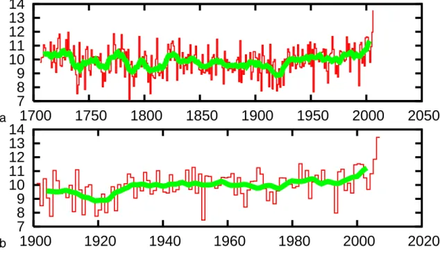
Meteorologically, the autumn of 2006 was an extraordinary season in Europe. In the Netherlands, the temperature averaged over September–November was 1.6◦C higher than the previous record, which was established in 2005 (Fig. 1). This is also 1.6◦C 25

(4)

CPD

3, 811–837, 2007

EGU larger than the uncertainties in the earlier part of the record. The Central England

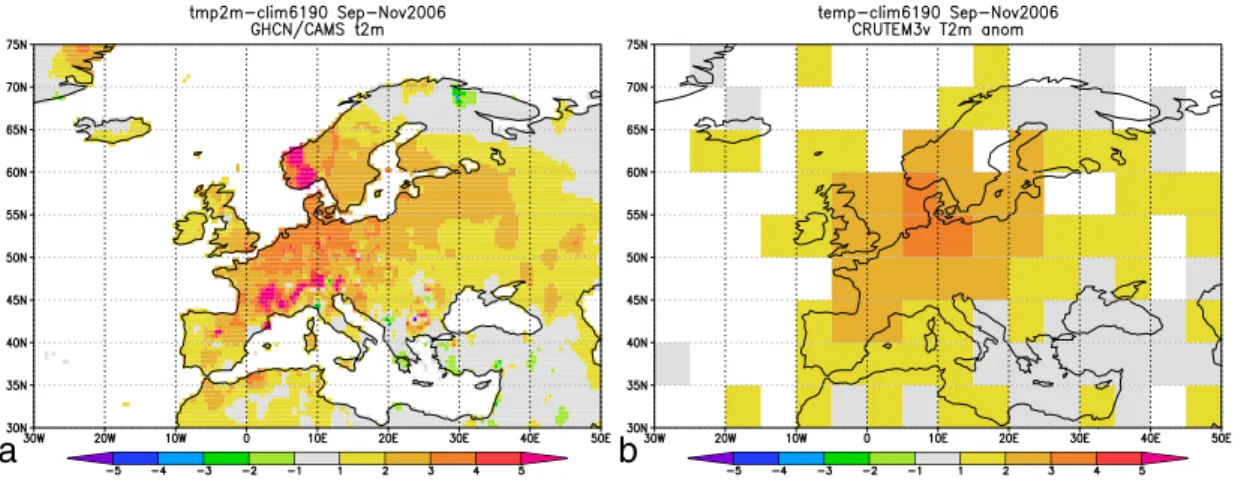
Temperature, 12.6◦C, also was the highest since the beginning of the measurements in 1659, 0.8◦C higher than the previous record of 1730 and 1731. Pinstrumental re-construction indicate that September–November 2006 was the warmest autumn since 1500 in a large part of Europe (Luterbacher et al., 2007). Figure 2 shows that the 5

observed temperatures from the 0.5◦ GHCN/CAMS dataset (Fan and van den Dool, 20071) exceeded the maximum over 1500–2002 (Xoplaki et al.,2005) by more than a degree in southeastern England, France, Belgium, the Netherlands, Germany and Switzerland.

The impacts of the high temperatures on society and nature have not been very 10

strong, as in autumn a higher temperature corresponds to a phase lag of the seasonal cycle. Flowering bulb farmers in the Netherlands were reported to have problems due to premature flowering. However, a similar anomaly in summer would have given rise to a heat wave analogous to the summer of 2003, which caused severe problems (e.g., Sch ¨ar and Jendritzky,2004).

15

In this article the heat anomaly of the autumn of 2006 in Europe is analysed. First the observations are shown and return times are computed under the obviously false assumption of a stationary climate. Next the first order effects of global warming are subtracted, and return time sof the remaining weather signal computed. The main weather factors are identified, and possible changes in their distribution are investi-20

gated using climate model simulations.

2 Observations

In Fig.1the time series of autumn (September–November) averaged temperature in De Bilt, the Netherlands is shown. This time series has been corrected for the

ef-1

Fan, Y. and van den Dool, H.: A global monthly land surface air temperature analysis for 1948-present, J. Geophys. Res., submitted, 2007.

(5)

CPD

3, 811–837, 2007

EGU fects of changes in thermometer hut, direct environment of the measurement location

(Brandsma and van der Meulen,2007a,b), and the effects of the growth of the cities in the area (Brandsma et al.,2003). The value for 2006 is seen to be well outside the distribution defined by the other years.

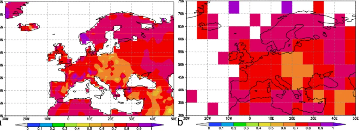
Figure 3shows two extrapolations of the distribution of the observed values 1901– 5

2005. The extrapolation and the return values are based on the obviously false as-sumption that all variability is interannual. The return times of 10000 years or more show that the climate does change on longer time scales. Global warming has made high temperatures much more likely during recent years, and this and other long-term variations decrease the number of degrees of freedom and hence increase the proba-10

bility of clustered high extremes.

The same analysis has been applied to all grid points of the 0.5◦GHCN/CAMS and 5◦CRUTEM3 (Brohan et al.,2006) datasets. The GHCN and CAMS time series used in the construction of the former have not been homogenised, in contrast to the De Bilt series of Figs.1,3(which is not included in this dataset). Inhomogeneous series show 15

up as isolated patches in the plots. The CRUTEM3 dataset uses more homogeneous data, at the expense of a much lower resolution.

Figure 4 shows that the area with 3◦C anomalies stretches from the north side of the Alps to Denmark and from Belgium to Poland, with a maximum at the north side of the Alps visible in the high-resolution dataset. A conservative extrapolation using 20

a Gaussian fit (Fig. 5) shows that in an unchanging climate the return times of this autumn would be 10 000 years or more in an area shifted somewhat to the west of the area with highest anomalies. The shift is due to the smaller variability near the Atlantic Ocean.

3 Global warming

25

The climate is not stationary: temperature have been rising over Europe as in most of the rest of the world. The effect of this on the probability of the occurrance of an

(6)

CPD

3, 811–837, 2007

EGU anomaly like in autumn 2006 can be studied by taking out the local temperature rise

proportional to global warming: T′_{(t) = AT}′

global(t) + ǫ(t) , (1)

where ǫ(t) denotes the part of the temperature not directly proportional to global warm-ing. The coefficients A are determined by a fit of local to global temperature up to 2005 5

and are shown in Fig.6.

Station inhomogeneities are clearly visible in the GHCN/CAMS dataset, these have been accounted for better in the much coarser CRUTEM3 dataset. On average the temperature in Europe has increased somewhat faster than the globally averaged tem-perature in autumn, in accordance with the Cold Ocean/Warm Land pattern (Sutton 10

et al.,2007).

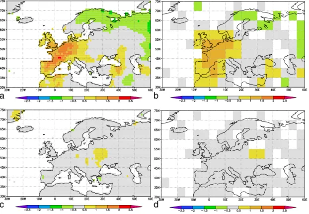
Subtracting the local trend AT_global′ (t) from the observed temperatures, the weather anomalies ǫ(t) remain. These are by definition not linearly related to global warming. In Fig.7the return period of the autumn 2007 De Bilt value is extrapolated. The central value of the more conservative Gaussian extrapolation is 650 years, with a lower bound 15

of the 95% CI of 250 year.

The same extrapolation in the GHCN/CAMS and CRUTEM3 datasets (Fig.8) show the improbable weather to have extended over a large part of Europe, with return times of ǫ(t) longer than 200 years over most of the area where the anomaly was largest, reaching 1000 years in northern Germany.

20

We conclude that global warming has made a temperature anomaly like the one observed in autumn 2006 between 10 and 50 times more likely than under the false assumption of stationary climate, with the larger factors near coasts where the trend is larger compared to natural variability. Still, other factors than global warming con-spired to give estimated return times well over 200 years in most of the area with large 25

anomalies, reaching 1000 years in northern Germany. A rare event indeed, even in a linearly warming climate.

(7)

CPD

3, 811–837, 2007

EGU

4 Circulation

Apart from global warming, temperature anomalies in Europe are determined to a large extend by circulation anomalies and sunshine. In the very simple model (VSM) ofvan Ulden and van Oldenborgh (2006) the anomaly in local monthly mean 2 m temperature is therefore decomposed as

5

T′_{(t) = T}′

circ+ Tnoncirc′ (t) + MT′(t − 1) (2)

T′

circ= AWG′west(t) + ASG_south′ (t) + BQ′sw(t) (3)

T′

noncirc(t) = AT ′

global(t) + η(t) . (4)

The circulation-dependent temperature anomalies T_circ′ are assumed to be linearly pro-portional to the zonal and meridional geostrophic wind anomalies G_west′ and G_south′ 10

and a measure for cloudiness, the net surface short-wave radiation Q′sw. (All

anoma-lies are relative to the mean observed values for 1961–1990.) The non-circulation-dependent temperature anomalies T_noncirc′ (t) consist of the part linearly proportional to global warming and the remaining noise η(t). Finally, M is a memory term for past circulations. This term is modelled as a regression on the previous months’ anomalous 15

temperature. The geostrophic winds are computed from the NCEP/NCAR reanalysis sea-level pressure (Kalnay et al.,1996).

There is some ambiguity in this model if the climate change involves changes in the circulation patterns parametrized by the geostrophic wind. However, the interannual variations in circulation are always much larger than the long-term shifts, so that in 20

practice the terms A_S, A_W, B are fixed by the interannual variability and this part of climate change is not contained in the circulation-independent temperature changes.

Averaged over the autumn, the coefficients AW and As reflect the gradients in the

cli-matological temperature over Europe (Fig.9). In this season the southerly component is most important in determining the temperature. More sunshine still has a positive 25

influence on temperature in Central Europe, but in northern Europe a lack of clouds increases night-time radiation more and hence cools the surface. The memory term

(8)

CPD

3, 811–837, 2007

EGU is large near seas due to the thermal inertia of sea water on the monthly time scale.

The small negative values in Central Europe show that in this region, circulation be-ing equal, a warm (and dry) August is slightly more likely to be followed by a cooler September. Apparently smaller persistence because of the dry soils accelerates the season cycle there.

5

The VSM Eqs. (2–4) explains over half the variance of the temperature, i.e., the cor-relation between the modelled temperature with η(t)=0 and the observed temperature is about r=0.7 to 0.8 in autumn in Europe (Fig.10).

In Fig.11the contribution of the various terms in the VSM are shown. The anoma-lous circulation contributed about 1.5◦C to the observed anomaly within the linear 10

framework of Eqs. (2–4). The large amount of sunshine in September increased the temperature by less than 0.5◦C in the seasonal average.

A persistent low-pressure area over the Atlantic Ocean caused predominantly south-easterly winds in September, southerly winds in October and south-westerly winds in November to the area north of the Alps (Fig. 12). In each of these months this 15

correponded to the direction with the highest temperatures.

On the shores of the North Sea persistence has also contributed. However, this was not due to the below-normal temepratures in August. The North Sea was still warm from the exceptionally high temperatures in July. This is not captured by the VSM, hence we cannot give a quantitative estimate. Based on the observed SST anomalies 20

of about 2◦C at the beginning of September it is estimated that this contributed roughly half a degree to the autumn temperature anomaly in De Bilt.

5 Climate model simulations

Observed autumn temperatures are far out of the range observed so far, even after linearly correcting for global warming. Do current climate models predict this type of 25

events to happen more frequently as Europe heats up? There are two caveats when using these models:

(9)

CPD

3, 811–837, 2007

EGU 1. the midlatitude circulation response of climate models varies greatly from model

to model and up to now lacks a sound theoretical footing (van Ulden and van Oldenborgh,2006;Miller et al.,2006);

2. the local temperature response to global warming is uncertain.

To investigate the changes in the distribution of autumn temperatures results from 5

the 17 standard runs with the ECHAM5/MPI-OM1 model (Jungclaus et al.,2006) runs of the ESSENCE project (Sterl et al., 20072) were used. These cover the period 1950– 2100 using observed concentrations of greenhouse gases and aerosols up to 2000 and the SRES A1B scenario afterwards. This model simulates the mean circulation over Europe reasonable well on monthly time scales (van Ulden and van Oldenborgh, 10

2006;van den Hurk et al.,2006).

An estimate of the systematic errors is provided by a comparison with results from the World Climate Research Programme’s (WCRP’s) Coupled Model Intercomparison Project phase 3 (CMIP3) multi-model dataset. Other models that simulate a reasonable mean climate over Europe are GFDL CM2.1 (Delworth et al.,2006), MIROC 3.2 T106 15

(K-1 model developers,2004), HadGEM1 (Johns et al.,2004) and CCCMA CGCM 3.2 T63 (Kim et al.,2002). The MIROC high resolution model did not have enough data to reconstruct changes in the full temperature distribution, only the mean.

The ECHAM5/MPI-OM model used in ESSENCE simulates the global mean tem-perature very well, with a ratio between observed and modelled trends of 1.10±0.07 20

(1σ errors). The GFDL CM2.1 model has similar agreement, but the other models overestimate the trend in the global mean temperature over 1950–2006 by factors 1.5 (HadGEM1), 1.6 (MIROC) and 2.0 (CCCMA). To account for these biases, we defined the local trend as a regression against modelled global mean temperature, as was done invan den Hurk et al. (2006). The local temperature rise as a function of time 25

2

Sterl, A., Severijns, C., van Oldenborgh, G. J., et al.: The ESSENCE project, in preparation, 2007.

(10)

CPD

3, 811–837, 2007

EGU rather than global mean temperature is higher by the same factors 1.5 to 2.0 in these

models.

Figure 13 shows the ratio of observed and modelled warming trends in Europe in autumn. The ECHAM5/MPI-OM model is seen to underestimate the warming trend in the area of the observed extreme by a factor 1.5 or more. In the other models the 5

ratio between local observed and modelled temperature trends has larger errors as there are fewer ensemble members available, but these models also show a higher observed than modelled warming relative to the rest of the world in the areas of the autumn 2006 anomaly.

Figure14shows the extreme value distribution of the ECHAM5/MPI-OM model sur-10

face air temperature at the position of De Bilt for different 30-year intervals. Above the linear increase in temperature proportional to the global mean temperature rise, there is no indication of any change in the distribution that would make extremely warm autumn temperatures more likely. In summer this change is clearly seen by steeper slopes in the cumulative ditributions (not shown); this can be understand from soil 15

moisture effects (e.g.,Sch ¨ar and Jendritzky,2004;Seneviratne et al.,2006).

This result was confirmed for the other climate models with a reasonable circulation over Europe for which a comparison between the 22nd and 23rd century with the 20th century could be made. None of these show an increase in the slope of the cumulative distribution at the grid point corresponding to De Bilt, Fig.15.

20

6 Conclusions

Apart from global warming, the anomalously high temperatures in Euope in autumn 2006 were caused by a persistent southerly wind direction advecting warm air to the north, more sunshine than normal, and persistence from the very hot July along the shores of the North Sea. Global warming has made a warm autumn like the one 25

observed in 2006 much more likely by shifting the temperature distribution to higher values. Taking this mean warming into account, the return time of the observed

(11)

tem-CPD

3, 811–837, 2007

EGU peratures in 2006 still is more than 200 years in large parts of Europe.

Current climate models underestimate the observed mean warming in Europe rel-ative to global warming. They also do not show an extra increase of the warm tail of the distribution as the climate warms. This means that we either observed a very rare event in 2006, or the current climate models lack some non-linear physics that causes 5

an underestimation of the impact of climate change on warm events in autumn.

Acknowledgements. I would like to thank my colleagues at KNMI for helpful comments. This

work was partly supported by the European Commission’s 6th Framework Programme project ENSEMBLES (contract number GOCE-CT-2003-505539). The ESSENCE project, lead by W. Hazeleger (KNMI) and H. Dijkstra (UU/IMAU), was carried out with support of DEISA, HLRS,

10

SARA and NCF (through NCF projects NRG-2006.06, CAVE-06-023 and SG-06-267). We thank the DEISA Consortium (co-funded by the EU, FP6 projects 508830/031513) for support within the DEISA Extreme Computing Initiative (http://www.deisa.org). I thank A. Sterl (KNMI), C. Severijns (KNMI), and HLRS and SARA staff for technical support. We acknowledge the other modeling groups for making their simulations available for analysis, the Program for

Cli-15

mate Model Diagnosis and Intercomparison (PCMDI) for collecting and archiving the CMIP3 model output, and the WCRP’s Working Group on Coupled Modelling (WGCM) for organizing the model data analysis activity. The WCRP CMIP3 multi-model dataset is supported by the Office of Science, U.S. Department of Energy.

References

20

Brandsma, T. and van der Meulen, J. P.: Thermometer Screen Intercomparison in De Bilt (the Netherlands), Part I: Understanding the weather-dependent temperature differences, Int. J. Climatol., accepted, 2007a. 814

Brandsma, T. and van der Meulen, J. P.: Thermometer Screen Intercomparison in De Bilt (the Netherlands), Part II: Description and modeling of mean temperature differences and

25

extremes, Int. J. Climatol., accepted, 2007b. 814

Brandsma, T., K ¨onnen, G. P., and Wessels, H. R. A.: Estimation of the effect of urban heat advection on the temperature series of De Bilt (The Netherlands), Int. J. Climatol., 23, 829– 845, 2003.814

(12)

CPD

3, 811–837, 2007

EGU

Brohan, P., Kennedy, J., Haris, I., Tett, S. F. B., and Jones, P. D.: Uncertainty estimates in regional and global observed temperature changes: a new dataset from 1850, J. Geophys. Res., 111, D12106, doi:10.1029/2005JD006548, 2006. 814

Delworth, T. L., Broccoli, A. J., Rosati, A., Stouffer, R. J., Balaji, V., Beesley, J. A., Cooke, W. F., Dixon, K. W., Dunne, J., Dunne, K. A., Durachta, J. W., Findell, K. L., Ginoux, P.,

5

Gnanadesikan, A., Gordon, C. T., Griffies, S. M., Gudgel, R., Harrison, M. J., Held, I. M., Hemler, R. S., Horowitz, L. W., Klein, S. A., Knutson, T. R., Kushner, P. J., Langenhorst, A. R., Lee, H. C., Lin1, S. J., Lu, J., Malyshev, S. L., Milly, P. C. D., Ramaswamy, V., Russell, J., Schwarzkopf, M. D., Shevliakova, E., Sirutis, J. J., Spelman, M. J., Stern, W. F., Winton, M., Wittenberg, A. T., Wyman, B., Zeng, F., and Zhang, R.: GFDL’s CM2 global coupled

10

climate models – Part 1: Formulation and simulation characteristics, J. Climate, 19, 643– 674, doi:10.1175/JCLI3629.1, 2006. 818

Johns, T., Durman, C., Banks, H., Roberts, M., McLaren, A., Ridley, J., Senior, C., Williams, K., Jones, A., Keen, A., Rickard, G., Cusack, S., Joshi, M., Ringer, M., Dong, B., Spencer, H., Hill, R., Gregory, J., Pardaens, A., Lowe, J., Bodas-Salcedo, A., Stark, S., and Searl, Y.:

15

HadGEM1 — Model description and analysis of preliminary experiments for the IPCC Fourth Assessment Report, Tech. Rep. 55, U.K. Met Office, Exeter, UK, 2004. 818

Jungclaus, J. H., Keenlyside, N., Botzet, M., Haak, H., Luo, J.-J., Latif, M., Marotzke, J., Mikola-jewicz, U., and Roeckner, E.: Ocean circulation and tropical variability in the coupled model ECHAM5/MPI-OM, J. Climate, 19, 3952–3972, doi:10.1175/JCLI3827.1, 2006. 818

20

K-1 model developers: K-1 coupled model (MIROC) description, Tech. Rep. 1, Center for Cli-mate System Research, University of Tokyo, 2004. 818

Kalnay, E., Kanamitsu, M., Kistler, R., Collins, W., Deaver, D., Gandin, L., Iredell, M., Saha, S., White, G., Woollen, J., Zhu, Y., Leetma, A., Reynolds, R., Chelliah, M., Ebisuzaki, W., Higgens, W., Janowiak, J., Mo, K. C., Ropelewski, C., Wang, J., and Jenne, R.: The

25

NCEP/NCAR 40-year reanalysis project, Bull. Amer. Meteorol. Soc., 77, 437–471, 1996.

816

Kim, S.-J., Flato, G. M., de Boer, G. J., and McFarlane, N. A.: A coupled climate model simu-lation of the Last Glacial Maximum, Part 1: transient multi-decadal response, Climate Dyn., 19, 515–537, 2002.818

30

Luterbacher, J., Liniger, M. A., Menzel, A., Estrella, N., Della-Marta, P. M., Pfister, C., Rutishauser, T., and Xoplaki, E.: The exeptional European warmth of Autumn 2006 and Win-ter 2007: Historical context, the underlying dynamics and its phenological impact, Geophys.

(13)

CPD

3, 811–837, 2007

EGU

Res. Lett., accepted, 2007.

Miller, R. L., Schmidt, G. A., and Shindell, D. T.: Forced annular variations in the 20th century IPCC AR4 simulations, J. Geophys. Res., 111, D18101, doi:10.1029/2005JD006323, 2006.

818

Sch ¨ar, C. and Jendritzky, G.: Hot news from summer 2003, Nature, 432, 559–560, 2004.813,

5

819

Seneviratne, S. I., Luthi, D., Litschi, M., and Sch ¨ar, C.: Land ˆA-atmosphere coupling and climate change in Europe, Nature, 443, 205–209, doi:10.1038/nature05095, 2006. 819

Sutton, R. T., Dong, B.-W., and Gregory, J. M.: Land/sea warming ratio in response to climate change: IPCC AR4 model results and comparison with observations, Geophys. Res. Lett.,

10

34, L02701, doi:10.1029/2006GL028164, 2007. 815

van den Hurk, B. J. J. M., Klein Tank, A. M. G., Lenderink, G., van Ulden, A. P., van Oldenborgh, G. J., Katsman, C. A., van den Brink, H. W., Keller, F., Bessembinder, J. J. F., Burgers, G., Komen, G. J., W., H., and Drijfhout, S. S.: KNMI Climate Change Scenarios 2006 for the Netherlands, Tech. Rep. WR-2006-01, KNMI, 2006. 818

15

van Ulden, A. P. and van Oldenborgh, G. J.: Large-scale atmospheric circulation biases and changes in global climate model simulations and their importance for climate change in Cen-tral Europe, Atmos. Chem. Phys., 6, 863–881, 2006. 816,818

Xoplaki, E., Luterbacher, J., Paeth, H., Dietrich, D., N., S., Grosjean, M., and Wanner, H.: European spring and autumn temperature variability and change of extremes over the last

20

(14)

CPD

3, 811–837, 2007

Printer-friendly Version Interactive Discussion EGU a

7

8

9

10

11

12

13

14 1700

1750

1800

1850

1900

1950

2000

2050

b

7

8

9

10

11

12

13

14 1900

1920

1940

1960

1980

2000

2020

Fig. 1. Autumn temperatures at De Bilt, the Netherlands with a 10-yr running mean (green)

1706–2006 (a), 1901–2006 corrected for changes in the thermometer hut, location and city effects (b).

(15)

CPD

3, 811–837, 2007

EGU Fig. 2. The observed temperature in September–November 2007 minus the maximum

(16)

CPD

3, 811–837, 2007

Printer-friendly Version Interactive Discussion EGU 7 8 9 10 11 12 13 14 10000 1000 100 10 5 2 [Celsius]

return period [yr]

Sep-Nov homogenized temperature De Bilt 1901:2005

gauss fit gpd fit 2006

Fig. 3. Extrapolation of De Bilt autumn temperatures 1901–2005 (crosses) to the value

ob-served in 2006 (horizontal line). The return times have been computed under the obviously false assumption of only interannual variability. The upper and lower lines indicate the 95% CI, determined with a non-parametric bootstrap.

(17)

CPD

3, 811–837, 2007

EGU

a b

Fig. 4. The temperature anomaly (relative to 1961–1990) of September–November 2006 in the

(18)

CPD

3, 811–837, 2007

EGU

a b

Fig. 5. The return time of September–November 2006 in the GHCN/CAMS dataset 1948–

2005 (a) and the CRUTEM3 dataset 1901–2005 (b) under the false assumption of a stationary climate.

(19)

CPD

3, 811–837, 2007

EGU

a b

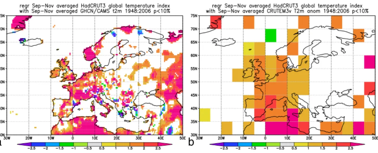
Fig. 6. The regression of local against globally averaged temperature over 1948–2006 in the

GHCN/CAMS (a) and CRUTEM3 (b) datasets. Only grid points where the correlation is 90% signficant are shown.

(20)

CPD

3, 811–837, 2007

Printer-friendly Version Interactive Discussion EGU 7 8 9 10 11 12 13 14 10000 1000 100 10 5 2 [Celsius]

return period [yr]

Sep-Nov Tdebilt - 1.68 Tglobal 1901:2005

gpd fit gauss fit 2006

Fig. 7. As Fig.3but now with 1.68 times the global mean temperature anomalies (with a 3 yr running mean) subtracted.

(21)

CPD

3, 811–837, 2007

EGU

a b

Fig. 8. As Fig.3but now with the local linear regression against the global mean temperature anomalies (with a 3 yr running mean, Fig.6) subtracted.

(22)

CPD

3, 811–837, 2007

EGU

a b

c d

Fig. 9. The coefficients of the VSM Eqs. (2–4) averaged over September–November: zonal geostrophic wind A_W[Km−1s] (a), the meridional zonal wind A_S[Km−1s] (b), the solar radiation

B[KW−1_m2

(23)

CPD

3, 811–837, 2007

EGU

a b

Fig. 10. Correlation of the September–November temperature anomaly from the VSM with η(t) = 0 and the observed temperature 1948–2006 for the GHCN/CAMS (a) and the CRUTEM3v (b) datasets.

(24)

CPD

3, 811–837, 2007

EGU

a b

c d

Fig. 11. Contribution of the circulation term (a, b) and solar radiation term (c, d) to the

(25)

CPD

3, 811–837, 2007

EGU

a b c

Fig. 12. NCEP/NCAR sea-level pressure anomalies in September (a), October (b) and

(26)

CPD

3, 811–837, 2007

EGU

a _b _c

d e

Fig. 13. Ratio of observed and modelled trends 1950-2006. ESSENCE (ECHAM5/MPI-OM) (a), GFDL CM2.1 (b), MIROC 3.2 T106 (c), UKMO HadGEM1 (d) and CCCMA CGCM3.1 T63 (e). Only grid points where the difference with one is at least one standard error are shown.

(27)