Improved correction for non-photochemical quenching of in situ chlorophyll fluorescence based on a synchronous irradiance profile

HAL Id: hal-01884903

https://hal.sorbonne-universite.fr/hal-01884903

Submitted on 1 Oct 2018

HAL is a multi-disciplinary open access archive for the deposit and dissemination of sci-entific research documents, whether they are pub-lished or not. The documents may come from teaching and research institutions in France or abroad, or from public or private research centers.

L’archive ouverte pluridisciplinaire HAL, est destinée au dépôt et à la diffusion de documents scientifiques de niveau recherche, publiés ou non, émanant des établissements d’enseignement et de recherche français ou étrangers, des laboratoires publics ou privés.

Distributed under a Creative Commons Attribution| 4.0 International License

irradiance profile

Xiaogang Xing, Nathan Briggs, Emmanuel Boss, Hervé Claustre

To cite this version:

Xiaogang Xing, Nathan Briggs, Emmanuel Boss, Hervé Claustre. Improved correction for non-photochemical quenching of in situ chlorophyll fluorescence based on a synchronous irradiance pro-file. Optics Express, Optical Society of America - OSA Publishing, 2018, 26 (19), pp.24734-24751. �10.1364/OE.26.024734�. �hal-01884903�

Improved correction for non-photochemical

quenching of

in situ

chlorophyll fluorescence

based on a synchronous irradiance profile

X

X

,

N

B

,

E

B

,

H

C

1_{State Key Laboratory of Satellite Ocean Environment Dynamics (SOED), Second Institute of}

Oceanography, State Oceanic Administration, Hangzhou 310012, China

2_{National Oceanography Centre Southampton, University of Southampton, Southampton SO14 3ZH, UK} 3_{School of Marine Sciences, University of Maine, 706 Aubert Hall, Orono, ME 04469, USA}

4_{Sorbonne Université, CNRS, Laboratoire d'Océanographie de Villefranche (LOV),}

Villefranche-sur-Mer F-06230, France

*xing@sio.org.cn

Abstract: In situ chlorophyll fluorometers have been used to quantify the distribution of

chlorophyll concentration in natural waters for decades. However, chlorophyll fluorescence is depressed during daylight hours due to non-photochemical quenching (NPQ). Corrections attempted to date have provided improvement but still remain unsatisfactory, often over-estimating the expected value. In this study, we examine the relationship between NPQ and instantaneous Photosynthetically Active Radiation (iPAR) using field data from BGC-Argo floats equipped with Chlorophyll-a fluorometers and radiometers. This analysis leads to an improved NPQ correction that incorporates both iPAR and mixed layer depth (MLD) and is validated against data collected at sunrise or sunset. The optimal NPQ light threshold is found to be iPAR = 15 μmol quanta m−2 _s−1_{, and the proposed methods based on such a light}

threshold correct the NPQ effect more accurately than others, except in “shallow-mixing” waters (NPQ light threshold depth deeper than MLD). For these waters, an empirical-relationship-based method is proposed for improvement of NPQ correction using an iPAR profile. It is therefore recommended that, for optimal NPQ corrections, profiling floats measuring chlorophyll fluorescence in daytime be equipped with iPAR radiometers.

Published by The Optical Society under the terms of the Creative Commons Attribution 4.0 License. Further distribution of this work must maintain attribution to the author(s) and the published article’s title, journal citation, and DOI.

OCIS codes: (010.4450) Oceanic optics; (120.4640) Optical instruments.

References and links

1. C. Lorenzen, “A method for the continuous measurement of in vivo chlorophyll concentration,” Deep-Sea Res. 13, 223–227 (1966).

2. T. Platt, “Local phytoplankton abundance and turbulence,” Deep-Sea Res. 19, 183–187 (1972).

3. J. J. Cullen, “The deep chlorophyll maximum: comparing vertical profiles of chlorophyll a,” Can. J. Fish. Aquat. Sci. 39(5), 791–803 (1982).

4. E. Boss, D. Swift, L. Taylor, P. Brickley, R. Zaneveld, S. Riser, M. J. Perry, and P. G. Strutton, “Observations of pigment and particle distributions in the western North Atlantic from an autonomous float and ocean color satellite,” Limnol. Oceanogr. 53(5), 2112–2122 (2008).

5. IOCCG, “Bio-Optical Sensors on Argo Floats,” Reports of the International Ocean-Colour Coordinating Group, No. 11, H. Claustre, ed. (2011).

6. K. Johnson and H. Claustre, “The scientific rationale, design and Implementation Plan for a Biogeochemical-Argo float array,” (2016).

7. C. W. Proctor and C. S. Roesler, “New insights on obtaining phytoplankton concentration and composition from in situ multispectral Chlorophyll fluorescence,” Limnol. Oceanogr. Methods 8, 695–708 (2010).

8. X. Xing, A. Morel, H. Claustre, D. Antoine, F. d’Ortenzio, A. Poteau, and A. Mignot, “Combined processing and mutual interpretation of radiometry and fluorimetry from autonomous profiling Bio-Argo floats: Chlorophyll a retrieval,” J. Geophys. Res. 116(C6), C06020 (2011).

9. H. Lavigne, F. d’Ortenzio, H. Claustre, and A. Poteau, “Towards a merged satellite and in situ fluorescence ocean chlorophyll product,” Biogeosci. 9(6), 2111–2125 (2012).

#334333

10. R. Sauzède, H. Claustre, C. Jamet, J. Uitz, J. Ras, A. Mignot, and F. d’Ortenzio, “Retrieving the vertical distribution of chlorophyll a concentration and phytoplankton community composition from in situ fluorescence profiles: A method based on a neural network with potential for global-scale applications,” J. Geophys. Res. 120(1), 451–470 (2015).

11. X. Xing, H. Claustre, E. Boss, C. Roesler, E. Organelli, A. Poteau, M. Barbieux, and F. d’Ortenzio, “Correction of profiles of in-situ chlorophyll fluorometry for the contribution of fluorescence originating from non-algal matter,” Limnol. Oceanogr. Methods 15(1), 80–93 (2017).

12. M. Behrenfeld and E. Boss, “Beam attenuation and chlorophyll concentration as alternative optical indices of phytoplankton biomass,” J. Mar. Res. 64(3), 431–451 (2006).

13. B. S. Sackmann, M. J. Perry, and C. C. Eriksen, “Seaglider observations of variability in daytime fluorescence quenching of chlorophyll-a in Northeastern Pacific coastal waters,” Biogeosciences Discuss. 5(4), 2839–2865 (2008).

14. X. Xing, H. Claustre, S. Blain, F. d’Ortenzio, D. Antoine, J. Ras, and C. Guinet, “Quenching correction for in vivo chlorophyll fluorescence acquired by autonomous platforms: A case study with instrumented elephant seals in the Kerguelen region (Southern Ocean),” Limnol. Oceanogr. Methods 10(7), 483–495 (2012).

15. A. Morel and D. Antoine, “Heating rate within the upper ocean in relation to its bio-optical state,” J. Phys. Oceanogr. 24(7), 1652–1665 (1994).

16. D. A. Kiefer, “Chlorophyll a fluorescence in marine centric diatoms: responses of chloroplasts to light and nutrients stress,” Mar. Biol. 23(1), 39–46 (1973).

17. J. Marra, “Analysis of diel variability in chlorophyll fluorescence,” J. Mar. Res. 55(4), 767–784 (1997). 18. R. M. Letelier, M. R. Abbott, and D. M. Karl, “Chlorophyll natural fluorescence response to upwelling events in

the Southern Ocean,” Geophys. Res. Lett. 24(4), 409–412 (1997).

19. M. Behrenfeld, T. Westberry, E. Boss, R. O’Malley, D. Siegel, J. Wiggert, B. Franz, C. McClain, G. Feldman, S. Doney, J. Moore, G. Dall’Olmo, A. Milligan, I. Lima, and N. Mahowald, “Satellite-detected fluorescence reveals global physiology of ocean phytoplankton,” Biogeosciences 6(5), 779–794 (2009).

20. H. Claustre, A. Morel, M. Babin, C. Cailliau, D. Marie, J.-C. Marty, D. Tailliez, and D. Vaulot, “Variability in particle attenuation and chlorophyll fluorescence in the tropical Pacific: Scales, patterns, and biogeochemical implications,” J. Geophys. Res. 104(C2), 3401–3422 (1999).

21. C. Roesler and A. H. Barnard, “Optical proxy for phytoplankton biomass in the absence of photophysiology: Rethinking the absorption line height,” Methods in Oceanography 7, 79–94 (2013).

22. S. J. Thomalla, W. Moutier, T. J. Ryan-Keogh, L. Gregor, and J. Schütt, “An optimized method for correcting fluorescence quenching using optical backscattering on autonomous platforms,” Limnol. Oceanogr. Methods 16, 132–144 (2017).

23. L. Biermann, C. Guinet, M. Bester, A. Brierley, and L. Boehme, “An alternative method for correcting fluorescence quenching,” Ocean Sci. 11(1), 83–91 (2015).

24. J. Plant, personal communications (2017).

25. K. E. Brainerd and M. C. Gregg, “Surface mixed and mixing layer depths,” Deep Sea Res. Part I Oceanogr. Res. Pap. 42(9), 1521–1543 (1995).

26. O. Holm-Hansen, A. F. Amos, and C. D. Hewes, “Reliability of estimating chlorophyll-a concentrations in Antarctic waters by measurement of in situ chlorophyll-a fluorescence,” Mar. Ecol. Prog. Ser. 196, 103–110 (2000).

27. C. de Boyer Montégut, G. Madec, A. S. Fischer, A. Lazar, and D. Iudicone, “Mixed layer depth over the global ocean: An examination of profile data and a profile-based climatology,” J. Geophys. Res. 109(C12), C12003 (2004).

28. G. Monterey and S. Levitus, “Seasonal variability of mixed layer depth for the World Ocean,” NOAA Atlas NESDIS 14, US Gov. Printing Office, Wash., D.C., 96 pp. (1997).

29. G. E. Kim, M.-A. Pradal, and A. Gnanadesikan, “Quantifying the biological impact of surface ocean light attenuation by colored detrital matter in an ESM using a new optical parameterization,” Biogeosciences 12(16), 5119–5132 (2015).

30. A. Morel, Y. Huot, B. Gentili, P. J. Werdell, S. B. Hooker, and B. A. Franz, “Examining the consistency of products derived from various ocean color sensors in open ocean (Case 1) waters in the perspective of a multi-sensor approach,” Remote Sens. Environ. 111(1), 69–88 (2007).

31. E. Organelli, H. Claustre, A. Bricaud, C. Schmechtig, A. Poteau, X. Xing, L. Prieur, F. D’Ortenzio, G.

Dall’Olmo, and V. Vellucci, “A novel near-real-time quality-control procedure for radiometric profiles measured by Bio-Argo floats: protocols and performances,” J. Atmos. Ocean. Technol. 33(5), 937–951 (2016).

32. C. Schmechtig, A. Poteau, H. Claustre, F. d’Ortenzio, G. Dall’Olmo, and E. Boss, “Processing Bio-Argo particle backscattering at the DAC level,” (2015).

33. C. Roesler, J. Uitz, H. Claustre, E. Boss, X. Xing, E. Organelli, N. Briggs, A. Bricaud, C. Schmechtig, A. Poteau, F. d’Ortenzio, J. Ras, S. Drapeau, N. Haëntjens, and M. Barbieux, “Recommendations for obtaining unbiased chlorophyll estimates from in situ chlorophyll fluorometers: A global analysis of WET Labs ECO sensors,” Limnol. Oceanogr. Methods 15(6), 572–585 (2017).

34. J. R. Taylor and R. Ferrari, “Shutdown of turbulent convection as anew criterion for the onset of spring phytoplankton blooms,” Limnol. Oceanogr. Methods 56(6), 2293–2307 (2011).

35. K. S. Johnson, J. N. Plant, L. J. Coletti, H. W. Jannasch, C. M. Sakamoto, S. C. Riser, D. D. Swift, N. L. Williams, E. Boss, N. Haentjens, L. D. Talley, and J. L. Sarmiento, “Biogeochemical sensor performance in the SOCCOM profiling float array,” J. Geophys. Res. 122(8), 6416–6436 (2017).

36. W. W. Gregg and K. L. Carder, “A simple spectral solar irradiance model for cloudless maritime atmospheres,” Limnol. Oceanogr. 35(8), 1657–1675 (1990).

37. A. Morel and S. Maritorena, “Bio-optical properties of oceanic waters: A reappraisal,” J. Geophys. Res. 106(C4), 7163–7180 (2001).

1. Introduction

Since in vivo fluorometry was introduced by Lorenzen in 1966 [1], advances in field-deployable sensor technology have led to the routine use of in situ chlorophyll fluorometers to quantify the chlorophyll a concentration ([Chla], mg m−3) in natural waters [2,3]. The rapid increase in number of Argo-style profiling floats equipped with chlorophyll fluorometers over the past decade [4–6] has led to in vivo fluorometry playing an increasing role in the study of phytoplankton dynamics and distributions. In the near future, the thousand-float planned Biogeochemical-Argo (BGC-Argo) fleet [6] is expected to provide more than 50,000 vertical profiles every year in the world’s ocean (assuming weekly profiling).

Despite the merits of in situ Chla sensors (small size, low power consumption, high measurement frequency, stability, and relatively low cost), it has been known for a long time that conversion from fluorescence to [Chla] requires a variety of corrections and assumptions [3]. Several studies have contributed methods to convert fluorescence to [Chla] [4,7–10], remove non-algal fluorescence interference [7,11], and address non-photochemical quenching (NPQ), a phenomenon whereby cells exposed to high light exhibit reduced fluorescence per unit of chlorophyll [12–14]. Among these issues, the NPQ effect still remains a significant challenge. The ability to obtain reliable (unbiased by NPQ) information on [Chla] is critical to study of ocean biology and biogeochemistry, as well as for better estimations of heat flux [15].

NPQ is a physiological mechanism that phytoplankton undertake to protect their photosynthetic apparatus from damage when exposed to high light [16]. Its effect is ubiquitous in natural waters, affecting sensor-induced Chla fluorescence [16,17] as well as sun-induced natural fluorescence [18,19]. NPQ results in fluorescence per unit of chlorophyll exhibiting significant temporal, spatial and vertical variability. Coincident with diurnal variations in solar illumination, the fluorescence signal of a chlorophyll fluorometer is generally lowest (greatest NPQ) near local noon and highest at nighttime [13,19,21]. Due to the decrease in daytime irradiance with depth, the NPQ depression is strongest near the surface and declines with depth. This effect can be noticed in well mixed waters where [Chla] is homogeneous within the mixed layer but where NPQ results in a “subsurface/deep fluorescence maximum (DFM)” [14].

Several strategies have been employed to correct for NPQ. Night-time measurements do not suffer from NPQ, so when night-time profiles are close in time and space, they can be used to directly replace or correct daytime fluorescence [22]. However, for most BGC-Argo float operations, a different correction is needed to accommodate the much longer intervals between day and night profiles or absence of night profiles (e.g. many floats profile only near local noon). While the previously proposed NPQ correction methods [13,14] work satisfactorily in many oceanic systems, some recent studies suggest that they over-correct [Chla] in surface layers of the Southern Ocean [23,24]. This over-correction may have two potential causes: erroneous estimation of actively mixing layer depth (XLD) due to the criterion used to define the mixed layer depth (MLD) [25], and/or lack of consideration of the minimum light intensity required to induce NPQ [26]. With respect to mixing, the two previous corrections proposed by [13] and [14] assumed an actively mixing mixed layer (XLD = MLD), using for MLD criterion the depth where density increases relative to the surface value by 0.03 kg m−3 _{or 0.125 kg m}−3 _{[27,28]. On the other hand, criteria defining}

In addition [13], and [14] did not consider the prevailing light intensity. Holm-Hansen et al. [26] have reported that the NPQ of Chla fluorescence appears when the Instantaneous Photosynthetically Available Radiation (iPAR) is greater than 40 μmol quanta m−2 _s−1 _{in the}

Southern Ocean. If iPAR measurements are available, incorporating such a “light-threshold” criterion as part of the NPQ correction scheme could potentially represent a useful alternative to circumvent the above over-correction problem; we explore such a “light-threshold” approach in this study.

Here, we analyze a data set from profiling floats that profile multiple times a day to determine the light and MLD thresholds for optimal NPQ correction. When the quenching depth exceeds the MLD, an empirical relationship between iPAR and NPQ is proposed to correct the NPQ not only above but also below the MLD. All the methods proposed are validated and compared with previous methods, by comparing BGC-Argo-measured fluorescence profiles acquired at noon with those acquired at sunrise or sunset, when no NPQ is assumed. Based on these analyses, recommendations are proposed to improve the quality control and correction procedures for fluorescence profiles acquired in aquatic environments, and in particular, but not exclusively, by BGC-Argo floats.

2. Materials and methods

2.1 NPQ correction methods

2.1.1 NPQ correction methods based on MLD

Two NPQ correction methods, hereafter denoted S08 and X12 [13,14], were developed and applied on data collected with Chla fluorometers deployed on profiling platforms (gliders and BGC-Argo floats) within the mixed layer:

= / bp. FRatio FChla b (1)

(

)

(

)

(

)

z z FRatio max FRatio z MLD≤ (2a)

(

)

(

(

)

)

FRatio z max FRatio z MLD≤ (2b)

( )

(

_{( )}

)

( ) (

)

(

)

(

)

(

)

z z FChla max FChla z MLD≤ (4a)

(

)

(

(

)

)

FChla z max FChla z MLD≤ (4b)

( )

(

_{( )}

) (

)

Here, FChla and S08/X12 stand for the uncorrected and NPQ-corrected FChla, respectively. bbp is the particle backscattering coefficient (generally measured at 700 nm), FRatio is the

FChla/bbp ratio. zMaxFluo and zMaxFRatio represent the depths where the uncorrected FChla and

the uncorrected FChla/bbp ratio reach their maximum value within the mixed layer,

respectively. Note that these two depths are, by definition, always shallower or equal to the MLD (Eq. (2) and 4).

Both methods extrapolate FChla into the upper part of the surface mixed-layer from depth based on the FChla at zMaxFluo (for X12) or the FRatio at zMaxFRatio (for S08). They rely on two

key assumptions: 1) the depth of the layer affected by NPQ is shallower than the MLD, and 2) either [Chla] (for X12) or FRatio (for S08) is uniformly distributed within the “NPQ layer”,

consistent with an a priori assumption that the mixed layer is an actively mixing layer. Consequently, either the maximal value of FChla (for X12) or the maximal FRatio (for S08) is assumed to correspond to the value not affected by NPQ, since NPQ always results in FChla depression. Both of the above assumptions can introduce errors, which the methods below are designed to reduce.

2.1.2 NPQ correction methods based on MLD and euphotic depth

Recently, a correction method [23] was proposed based on the use of the euphotic layer depth (zeu) instead of MLD, where zeu is the depth at which PAR reaches 1% of its surface value.

Where MLD > zeu, this method represents an improvement over a method based only on

MLD, because NPQ is not expected at zeu and below. The use of zeu can therefore improve

some cases of over-correction of NPQ discussed in Section 1 without introducing cases of under-correction. Furthermore zeu has a long history in oceanography as a light-threshold

horizon for photosynthesis, and many algorithms have been developed to compute it. [23] used an ocean-color-satellite-derived zeu, but satellite data is not always available, especially

during winter in high latitude regions. Plant et al. [24] updated this method with estimated diffused attenuation coefficient of PAR (i.e. Kd(PAR)) computed from uncorrected in situ

FChla based on an empirical relationship [29] (Eq. (6)). For comparison and discussion, their method, denoted as P18, is presented here:

(

)

[

]

(

)

(

)

(

)

_

(

)

(

)

(

)

(

)

z z FChla max FChla z≤ MLD z (8a)

( )

(

(

(

)

)

)

FChla z =max FChla z≤ MLD z (8b)

( )

( ) (

_{( )}

)

Here [Chla] uses uncorrected FChla after basic processing (See Section 2.3). We have tried

another empirical method for estimating Kd(PAR) from [Chla] using [30] and found zeu

estimated by P18 to be more accurate (closer to the in situ radiometer-measured zeu).

2.1.3 NPQ correction methods based on MLD and light-threshold depth

In the present study, we propose new NPQ correction methods similar to P18, but using an absolute light threshold instead of zeu. The optimal iPAR threshold is found at 15 μmol quanta

m−2 _s−1 _{(see below), and the improved NPQ correction methods, hereafter denoted as S08 +}

and X12 + , rely on the definition of an “NPQ layer” from the surface to min(MLD, ziPAR15):

(

)

(

)

(

)

(

)

S08+ min , iPAR15 .

z =z FRatio max FRatio z= ≤ MLD z (10a)

(

)

(

(

(

)

)

)

FRatio z =max FRatio z≤ MLD z (10b)

( )

(

_{( )}

)

( ) (

)

(

)

(

)

(

)

(

)

(

)

(

(

(

)

)

)

FChla z =max FChla z≤ MLD z (12b)

( )

(

_{( )}

) (

)

2.1.4 NPQ correction method based on an empirical relationship

The above methods are not expected to perform well in shallow-mixing waters, when NPQ also occurs below the MLD, because the FChla at the reference depth may be already quenched to some extent. Therefore, for shallow-mixing waters with ziPAR15 > MLD, we

propose a different NPQ correction, in which an empirical fit between iPAR and NPQ is used to correct FChla below the MLD. Additionally, the corrected FChla at 10 m is extrapolated to the surface to circumvent potential errors introduced in the near surface, where wave focusing can cause large fluctuations in in situ iPAR measurements [8]. A sigmoid function is used to model NPQ with three parameters: r, the fraction of fluorescence signal not affected by NPQ; iPARmid, the iPAR value with the greatest gradient in a sigmoid function; and e, the exponent

coefficient of a sigmoid function. These parameters are computed based on an empirical fit between our measurements of iPAR and the observed ratio quenched FChla to unquenched FChla. The new method is hereafter denoted XB18 and is computed as follows:

( )

( )

(

(

)

(

(

( )

)

)

)

(

)

(

)

FChla z r r iPAR z iPAR z

z z z  _{+ − + ≥}  =  _{= <}  (14) 2.2 Statistical metrics

Three statistical metrics are used to evaluate different NPQ correction methods: 1) Mean Absolute Error (MAE), which represents the absolute errors between the corrected values and reference values; 2) Mean Absolute Percentage Error (MAPE), which represents the relative errors; 3) and Mean Percentage Error (MPE), which represents the systematic relative bias. They are defined as:

1 1 . n i i i MAE P A n = =



( )



(

_{)( )}



Here, Pi represents the corrected value of FChla, Ai is the reference value of FChla without

NPQ, and n represents the number of samples. In this study, these metrics are used to assess the level of agreement between FChla profiles corrected using 6 different NPQ corrections and reference profiles measured at sunrise or sunset.

2.3 Data

To evaluate the NPQ correction methods, a data set consisting of FChla, bbp(700) and iPAR

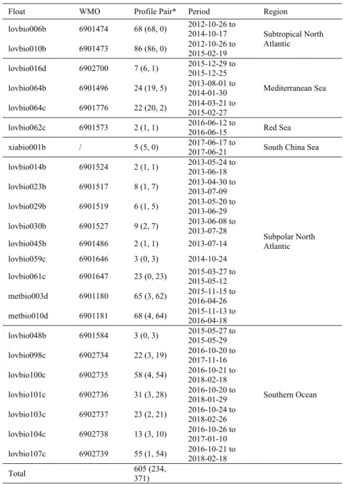
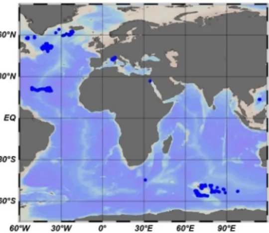
profiles collected by 23 profiling floats is used (Fig. 1, Table 1). 605 pairs of profiles (out of 850 in total) are selected for analysis according to the following criteria: 1) there are local noon and local sunrise/sunset profiles within a short time interval (<36 hours); 2) the mean absolute percentage difference (MAPE) of bbp(700) profiles from surface to 100m between

noon and sunrise/sunset is lower than 10% (this criterion caused most of the rejection of pairs); 3) if both the sunrise and sunset profiles satisfy the above requirements, then the profile with lower MAPE is chosen as reference. In this study, the sunrise or sunset profiles are assumed to exhibit no NPQ [16,20,21]. Additionally, we assume that any variation in [Chla] profiles between sunrise and noon (e.g. due to lateral and vertical advection or phytoplankton growth or grazing) is small compared to the effect of NPQ [12].

Table 1. Information related to BGC-Argo float data used in this study

Float WMO Profile Pair* Period Region

lovbio006b 6901474 68 (68, 0) 2012-10-26 to _{2014-10-17 Subtropical North} Atlantic lovbio010b 6901473 86 (86, 0) 2012-10-26 to _2015-02-19 lovbio016d 6902700 7 (6, 1) 2015-12-29 to _2015-12-25 Mediterranean Sea lovbio064b 6901496 24 (19, 5) 2013-08-01 to _2014-01-30 lovbio064c 6901776 22 (20, 2) 2014-03-21 to _2015-02-27

lovbio062c 6901573 2 (1, 1) 2016-06-12 to _2016-06-15 Red Sea xiabio001b / 5 (5, 0) 2017-06-17 to _2017-06-21 South China Sea lovbio014b 6901524 2 (1, 1) 2013-05-24 to _2013-06-18 Subpolar North Atlantic lovbio023b 6901517 8 (1, 7) 2013-04-30 to _2013-07-09 lovbio029b 6901519 6 (1, 5) 2013-05-20 to _2013-06-29 lovbio030b 6901527 9 (2, 7) 2013-06-08 to _2013-07-28 lovbio045b 6901486 2 (1, 1) 2013-07-14 lovbio059c 6901646 3 (0, 3) 2014-10-24 lovbio061c 6901647 23 (0, 23) 2015-03-27 to _2015-05-12 metbio003d 6901180 65 (3, 62) 2015-11-15 to _2016-04-26 metbio010d 6901181 68 (4, 64) 2015-11-13 to _2016-04-18 lovbio048b 6901584 3 (0, 3) 2015-05-27 to _2015-05-29 Southern Ocean lovbio098c 6902734 22 (3, 19) 2016-10-20 to _2017-11-16 lovbio100c 6902735 58 (4, 54) 2016-10-21 to _2018-02-18 lovbio101c 6902736 31 (3, 28) 2016-10-20 to _2018-01-29 lovbio103c 6902737 23 (2, 21) 2016-10-24 to _2018-02-26 lovbio104c 6902738 13 (3, 10) 2016-10-26 to _2017-01-10 lovbio107c 6902739 55 (1, 54) 2016-10-21 to _2018-02-18 Total 605 (234, ₃₇₁₎

* The numbers in the parentheses represent the number of profiles of the DCM- and w/oDCM-Type, respectively.

The mixed layer depth (MLD) is determined as the depth where the density is higher than its value at 10 m by 0.03 kg m−3 _{[27]. MLD is used to distinguish the DCM-Type profiles}

(without DCM). An analysis of the optimal MLD definition for NPQ correction is given in Section 3.2. The depth of maximum uncorrected FChla (DFM) is calculated first. The profiles with MLD shallower than DFM are identified as ‘DCM-Type’ (DFM is regarded as a true DCM), otherwise as ‘w/oDCM-Type’ (shallow DFM is assumed to be due to NPQ). Out of the 605 pairs, 234 are of ‘DCM-Type’, and 371 are of ‘w/oDCM-Type’ (Table 1).

Fig. 1. Locations of BGC-Argo floats used in this study.

All profiling floats used in this study are of the PROVOR CTS 4 series [31] equipped with a SeaBird CTD (SBE41CP), a Satlantic radiometer (OCR504) that measures downwelling irradiance at three wavelengths (380, 412 and 490 nm) and iPAR, and a WET Labs ECO Triplet that includes a Chla fluorometer (Ex/Em: 470nm/695nm), a backscattering sensor (700 nm), and a colored dissolved organic matter (CDOM) fluorometer (Ex/Em: 370nm/460nm) or, in few occasions, an additional backscattering sensor (532nm). The vertical resolution of the measurements is ~1 m from 250 m to 10 m and ~0.2 m from 10 m to the surface. The backscattering coefficient at 700 nm is processed following Schmechtig et al. [32]. Briefly, data are converted to engineering units, the contribution of salt water scattering is subtracted, and the backscattering coefficient is computed from the measurement of the volume scattering function at one angle. For Chla fluorometry, all the recorded fluorescence digital counts (DC) are converted to [Chla] using half of the factory calibration slope coefficient [33]. We find in certain cases that the application of a CDOM-interference correction [11] resulted in an over-correction (an abnormal increase of FChla at the surface), so the “deep-offset” correction method [11] is applied for dark current bias correction. The offset is determined as follows: 1) In each “deep” profile (defined as those profiles where maximal observation depth is deeper than 500m), the minimum FChla is determined; 2) all “minimum FChla” values are collected for each sensor; 3) the median value of minimum FChla observed by each sensor is taken as the reference offset for this sensor. This offset calculation is necessary (rather than using the factory dark counts, which are typically about 50 counts), due to a “float-sensor combination effect” which results in a dark signal change (typically ranging from 3 to 5 counts) when the sensor is mounted on the float.

3. Results and discussions

3.1 Choice of filter for smoothing FChla profiles

High frequency fluctuations in the FChla profiles negatively affect NPQ correction performance and need to be smoothed before any NPQ correction. In this study, we use a median filter as a low-pass filter to smooth out the high frequency fluctuations. However, if the filtering window is too small, it risks not removing enough of the fluctuations, leading to over-estimation of the maximum of FChla and FRatio. On the other hand, if filtering window

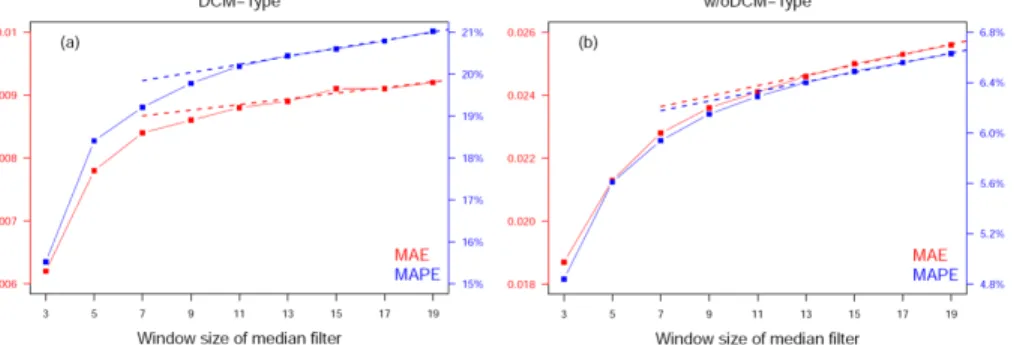
is too large, it will reduce true FChla maxima, under-estimating the maximum of FChla or FRatio. We therefore evaluate the optimal filtering window by studying the sensitivity of MAE and MAPE of median-filtered FChla values obtained when using different window size, taking the raw FChla as the reference, in w/oDCM- and DCM-Type waters, respectively (Fig. 2). MAE and MAPE in this context are used as measures of variability removed by the filter. As window size increases, there is initially substantial variability that is removed, exhibited by a large change in MAE and MAPE (Fig. 2). As the window size increases above 11 points, the improvement settles on a constant increase in MAE and MAPE for both water types. MAE due to random (Poisson) noise should not increase linearly with increasing filter width, so the linear portions of Fig. 2 suggest that further smoothing starts to eliminate nonrandom fluctuations (i.e., true features of the FChla profile). For the rest of this study, we thus choose to use an 11-point median window, representing a vertical resolution of ~11 m below 10 m depth and ~2 m above 10 m depth, and extrapolate the ending points (i.e., the first 5 values at surface, without enough filter window, are assigned as the median value of first 11 points).

Fig. 2. Mean Absolute Error (MAE) and Mean Absolute Percentage Error (MAPE) of median-filtered FChla values, taking the raw FChla as the reference, with the change of window size (from 3-point median to 19-point median) in DCM- (Panel a) and w/oDCM-Type (Panel b) waters, respectively. The dashed straight lines represent the linear regressed line between MAE/MAPE and the window size (from 13 to 19).

3.2 Optimizing the MLD criteria and ziPAR criteria for S08 + and X12 +

In this section, different MLD criteria and different ziPAR criteria are tested to determine the

optimal combination for NPQ correction. As mentioned above, the reported over-correction issue [23] may be due to 1) wrong estimation of actively mixing layer depth (XLD) when defining the mixed layer depth (MLD) [34], and/or 2) lack of consideration of a NPQ light threshold. For example, a very high gradient of chlorophyll located just below MLD can result in overcorrection if MLD is over-estimated. On the other hand, if XLD has shoaled recently, [Chla] is still homogeneous in the deeper ML, and NPQ extends below the XLD, then use of a shallower “MLD” criterion may lead to under-correction.

We assess statistically (using MAE, MAPE and MPE) the optimal MLD and ziPAR criteria

for NPQ correction by varying the MLD density criterion between 0.0025 to 0.03 kg m−3 _at

0.0025 kg m−3 _{increments and simultaneously varying the z}

iPAR criterion between 0 to 55

μmol quanta m−2 _s−1 _{at 5 μmol quanta m}−2 _s−1 _{increments (0 means no iPAR threshold is}

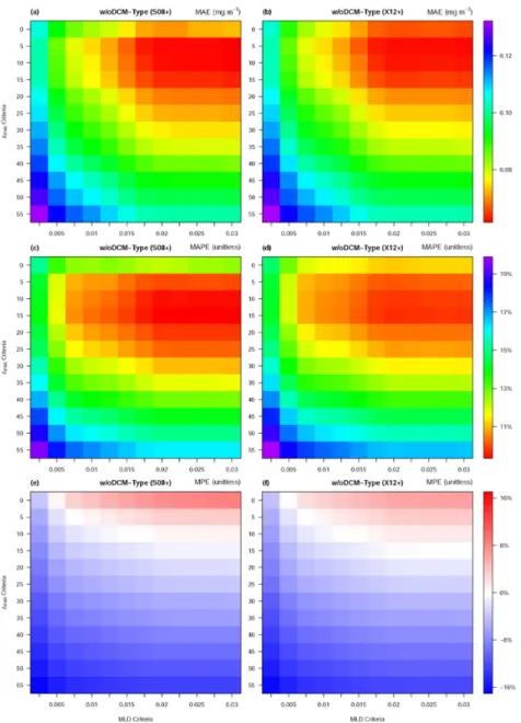
considered, so the results are just the original S08 and X12), for the w/oDCM-Type only (Fig. 3).

Surprisingly, the NPQ correction is found to be rather insensitive to MLD criterion once the criterion becomes larger than 0.015 kg m−3 _{(Fig. 3), suggesting that 1) for most cases,}

ziPAR is shallower than MLD0.015, and 2) the light threshold plays a dominant role in shaping

the NPQ correction, especially in deep mixing waters as found in the Southern Ocean. Best performance (lowest MAE and MAPE) occurs with higher density and lower light thresholds

(Fig. 3). MPE quantifies the systematical bias, with negative values denoting under-estimation and positive ones denoting over-under-estimation. Figure 3e and f display a clear change of MPE from the negative bias at the bottom left (ziPAR55 and MLD0.0025, the criterion with the

shallowest NPQ layer, very close to the uncorrected data) to the positive bias at the top right (i.e. ziPAR0 and MLD0.03, this criterion represents S08 and X12), with no systematic bias when

the light threshold is chosen at 10 or 15 μmol quanta m−2 _s−1_{. The optimal MLD criterion is in}

the range between 0.02 and 0.03 kg m−3_{, consistent with the MLD criterion of 0.03 kg m}−3

previously proposed [13-14]. This result confirms the strong benefit of adding light threshold to improve the NPQ correction.

Fig. 3. Analysis for ‘w/oDCM-Type’ waters: The variations of MAE (Mean Absolute Error), MAPE (Mean Absolute Percentage Error, right y-axis) and MPE (Mean Percentage Error) at different MLD criteria (x-axis) and different ziPAR criteria (y-axis) for the S08 + (left) and X12

Considering of all three metrics, we suggest that the optimal light threshold depth for NPQ correction could be chosen as ziPAR15, and that it is not necessary to change the MLD

criterion. Therefore, ziPAR15 and MLD0.03 are used in the light-threshold methods. Note that,

using the optimized definitions, mean values ( ± standard deviation) of MLD0.03 are 131 ( ±

86) m and 41 ( ± 27) m, and mean values ( ± standard deviation) of ziPAR15 are 103 ( ± 29) m

and 133 ( ± 30) m for the w/oDCM-Type and the DCM-Type, respectively. Hereafter, we use the abbreviation “MLD” to refer to MLD0.03.

3.3 Validation and comparison for w/o DCM-type

Fig. 4. Ratio of uncorrected FChla at noon to the reference vs. the noon iPAR value at the same depth (Panel a), as well as the corresponding P18 (Panel b), S08 (Panel c), X12 (Panel d), S08 + (Panel e) and X12 + ratios (Panel f), in the w/oDCM-Type waters. The colored curves represent the average values at the same iPAR, and dashed ones represent the standard deviations. The horizontal dashed lines represent the ratio = 1, and the vertical lines represent

iPAR = 15 μmol quanta m−2 _s−1_{, the numbers of points and profiles are listed in Table 2.}

Figure 4a illustrates the NPQ phenomenon in the w/oDCM-Type water with a significant depression of fluorescence signal at high irradiances. The NPQ magnitude can reach values as high as 90%, i.e., observed FChla at noon is only 10% of the value at the same depth at sunrise/sunset. A small over-correction (MPE of 10.0% and 6.8%) is exhibited by the S08 and X12 corrections [23] (Fig. 4c-d), most likely because FChla is larger near the bottom of the

MLD [23], due either to enhancement of phytoplankton biomass, increased intracellular [Chla] (faster than mixing), or significant differences between MLD and XLD (not an actively mixing layer); in such a case, both S08 and X12 over-estimate the MaxRatio or MaxFluo, resulting in an over-correction of the [Chla] profile. P18 represents an improvement compared to the previous methods (Fig. 4b) (MAE improves from 0.065 to 0.062 and MAPE improves from 11.5% to 10.6%), but it also exhibits the problem of over-correction (MPE of 4.7%), likely because zeu is often much deeper than the layer affected by

NPQ.

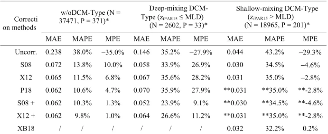
Table 2. Statistical results of all correction methods, taking the sunrise/sunset profiles as the reference. Correcti on methods w/oDCM-Type (N = 37471, P = 371)* Deep-mixing DCM-Type (ziPAR15≤ MLD) (N = 2602, P = 33)* Shallow-mixing DCM-Type (ziPAR15 > MLD) (N = 18965, P = 201)*

MAE MAPE MPE MAE MAPE MPE MAE MAPE MPE

Uncorr. 0.238 38.0% −35.0% 0.146 35.2% −27.9% 0.044 43.2% −29.3% S08 0.072 13.8% 10.0% 0.058 33.9% 26.9% 0.030 34.5% −4.6% X12 0.065 11.5% 6.8% 0.067 35.6% 28.2% 0.031 35.0% −2.8% P18 0.062 10.6% 4.7% 0.070 35.9% 27.9% **0.031 **35.0% **-2.8% S08 + 0.062 10.3% 1.3% 0.052 23.9% 9.1% **0.030 **34.5% **-4.6% X12 + 0.062 9.8% 1.0% 0.064 26.6% 11.2% **0.031 **35.0% **-2.8% XB18 / / / / / / 0.032 32.2% 0.2%

* N represents the sample size (number of points), and P represents the number of profiles ** Note that X12 + and P18 are identical to X12 and S08 + to S08 in Shallow-mixing DCM-Type

Compared to the earlier methods, the light-threshold methods proposed here perform better (Fig. 4(e) and 4(f)), with the ratio of noon to sunrise (or sunset) FChla closer to one. Statistically, all five methods have lower absolute errors (MAE) and relative errors (MAPE) values than the uncorrected FChla (Table 2), and the threshold-based methods (S08 + and X12 + ) are better than S08, X12 and P18 (Table 2), with MAPE improved from 10.6% (P18) to 9.8% (X12 + ), and MPE improved from 4.7% (P18) to 1.0% (X12 + ). There is no obvious difference between the two light-threshold methods and the very similar pattern between S08 and X12 is also seen in Figs. 4(c) and 4(d), suggesting that the backscattering has a negligible contribution to the improvement of NPQ correction, compared to the simpler extrapolation method solely based on FChla (i.e., X12 and X12 + ).

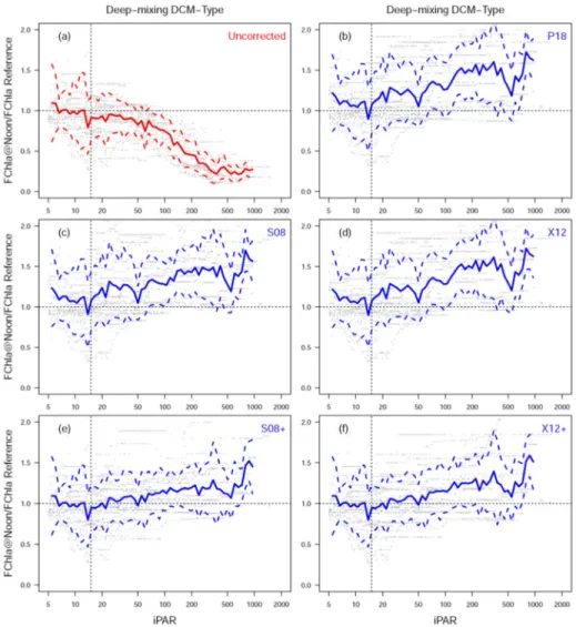
3.4 Validation for deep-mixing DCM-type (ziPAR15≤ MLD)

Based on the results of optimization analysis, all the DCM-Type profiles are further separated into two sub-types: Deep-mixing (ziPAR15 ≤ MLD, i.e. the light threshold is not deeper than

MLD and NPQ appears only in the mixed layer) and Shallow-mixing (ziPAR15 > MLD, i.e. the

light threshold is deeper than MLD and NPQ may occur below the mixed layer). Because S08 + and X12 + do not improve on S08 and X12 for the shallow mixing case, this case is addressed separately below.

For the Deep-mixing DCM-Type (Fig. 5), for which we have only 33 profiles, all the correction methods display a similar pattern to the w/oDCM-Type, including: 1) S08, X12 and P18 have an obvious over-correction with MPE ranging from 26.9% to 28.2%, and with MAPE larger than 33% (Table 2); 2) S08 + and X12 + show a significant improvement with MAPE lower than 27% and MPE lower than 12%, suggesting that light-threshold methods also work better than others in this case.

The proposed two methods using the absolute light intensity depth (ziPAR15) are superior to

P18 using zeu, although P18 does provide an improvement when compared to the original

vs. zeu in the NPQ correction is consistent with mechanistic understanding of NPQ. NPQ

depends on absolute light level [21], while zeu represents a relative light intensity. The depth

where NPQ effect is noticed (fluorescence signal depression magnitude) varies with daily light intensity rhythm and varies with depth (greater at surface and lower at depth, Fig. 4a and 5a), meanwhile, zeu is relatively stable at diurnal scale. Using an absolute light threshold (like

ziPAR15) is more consistent with the NPQ. We conclude that, for both w/oDCM-Type and

Deep-mixing DCM-Type, S08+/X12 + > P18 > S08/X12 (> means “an improvement compared to”). Note that we have also attempted to use a combined treatment method [7] to obtain [Chla] based on the downwelling irradiance (Ed(490)) profile, and use that to correct

NPQ effect of FChla. We found the method to introduce too much noise and be less robust than the method we have tested here.

Fig. 5. As same as Fig. 4, but for Deep-mixing DCM-Type (ziPAR15≤ MLD).

For floats without a radiometer we have tried an alternative NPQ-correction method based on the same theory of S08 + and X12 + , but using a modeled iPAR profile (See Appendix). It is intended for substituting S08 + & X12 + when the radiometry is unavailable, as well as for replacing P18, but results suggest that P18 outperforms the methods using modeled iPAR profile with lower MAE, MAPE and MPE and should therefore be used when measured iPAR

data is unavailable for now. Future work, using a more accurate estimation of surface iPAR, is likely to provide improvement.

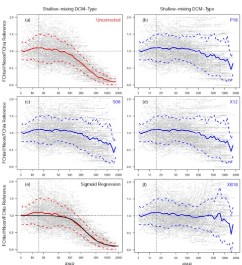
3.5 Validation for shallow-mixing DCM-type (ziPAR15 > MLD)

Fig. 6. Panel a-d are as same as Fig. 4, but for shallow-mixing DCM-Type (ziPAR15 > MLD).

Panel e shows the regressed sigmoid function between FChla ratio and iPAR, and Panel f shows the scatter plot of XB18

Figure 6a-d shows the same plot as Figs. 4 and 5, but for Shallow-mixing DCM-Type (ziPAR15

< MLD). The figures of S08 + and X12 + are not shown, as they are the same as S08 and X12, respectively. Note that P18 and X12 are also identical in this case. Although the uncorrected FChla still shows the quenching issue in high-light conditions (Fig. 6a), S08, X12 and P18 do not over-correct, but slightly under-correct (MPE as −4.6% and −2.8%) (Fig. 6b-d). It follows that if the layer impacted by NPQ is deeper than the mixed layer, all proposed methods cannot retrieve the correct FChla or FRatio for NPQ within the mixed layer, nor correct well for NPQ below the mixed layer. This is because in the stratified layer (below MLD) where NPQ is still occurring, we cannot assume that FChla or FRatio is constant with depth below MLD. In such cases, we propose a new method based on an empirical relationship between iPAR and NPQ (Fig. 6e; black line) following Eq. (14), using the following three empirical coefficients, r = 0.092, iPARmid = 261 μmol quanta m−2 s−1, and

Using this approach (XB18) there is no improvement in MAE, but MAPE decreases from 34.5% to 32.2%, and MPE becomes much closer to 0 (Table 2). It is noteworthy that the improvement is most significant under high irradiance conditions where the NPQ effect is greatest (Fig. 6f). For all points with iPAR > 100 μmol quanta m−2 _s−1_{, MAE, MAPE and}

MPE of XB18 are 0.027 mg m−3_{, 25.6% and −1.4%, respectively. Comparatively, the same}

metrics for P18 are 0.030 mg m−3_{, 38.9% and −12.5%, respectively.}

3.6 Simulation test for the low-resolution profiles

The present study is based on BGC-Argo data acquired with a vertical resolution of ~1m or better in the top 0-250 m layer. It is noteworthy that many BGC-Argo floats have lower vertical resolution, primarily in order to increase battery life. In this section, we test if the new methods proposed here (i.e. S08 + , X12 + and XB18) still represent an improvement when compared to S08, X12 and P18 under low-resolution observation.

The typical observation depths for an APEX float deployed as part of the SOCCOM project in the Southern Ocean are every 5m from 5 to 100 m, and every 10 m from 100 m to 360 m, every 20 m from 360 to 400 m, and every 50 m from 400 m to 1000 m [35]. The low-resolution noontime profiles are generated at SOCCOM depths by nearest neighbor interpolation of unsmoothed high-resolution profiles, and the low-resolution reference profiles are generated by linear interpolation of the smoothed high-resolution profiles. This choice is preferred because the reference values are used as the “true” unquenched (NPQ-corrected) profiles, and smoothing is necessary to remove the environmental noise. Before application of all NPQ correction methods, the simulated low-resolution noon data are smoothed by a 3-point median filter.

The final statistical results are shown in Table 3 (scatter plots are not shown). Note that the elimination of very high resolution data at z < 10 m also eliminates the most highly quenched data from this data set, so these statistics cannot be directly compared with the high resolution statistics in Tables 1 and 2. However, similar to the analysis based on high-resolution profiles (Table 2), the P18 method still represents a slight improvement over the previous S08 and X12 methods, and S08 + and X12 + still represent a further improvement in NPQ correction for w/oDCM-Type and Deep-mixing DCM-Type. In these waters, therefore, P18 is still the preferred method when iPAR is not measured, and X12 + is preferred when iPAR is measured. As for the Shallow-mixing DCM-Type, XB18 does not represent an unambiguous improvement over other methods when data are low resolution, unlike at high resolution, possibly because the improvement of XB18 relative to other methods is most pronounced near the surface.

Table 3. The same as Table 2, but for low vertical resolution data.

Correcti on methods

w/oDCM-Type _{Type (z}Deep-mixing

DCM-iPAR15≤ MLD)

Shallow-mixing DCM-Type (ziPAR15 > MLD)

MAE MAPE MPE MAE MAPE MPE MAE MAPE MPE Uncorr. 0.113 24.8% −17.1% 0.083 25.6% −16.1% 0.036 31.8% −11.8% S08 0.097 20.0% 16.5% 0.077 34.2% 24.7% 0.033 29.3% 1.0% X12 0.075 14.3% 10.3% 0.077 36.3% 27.4% 0.033 29.3% 1.4% P18 0.074 13.9% 9.6% 0.077 36.3% 27.4% *0.033 *29.3% *1.4% S08 + 0.072 13.2% 4.1% 0.069 25.5% 12.5% *0.033 *29.3% *1.0% X12 + 0.067 11.4% 2.8% 0.074 27.9% 14.2% *0.033 *29.3% *1.4% XB18 / / / / / / 0.033 28.7% 6.7%

4. Summary and recommendations

4.1 Summary

1) The methods S08 + and X12 + , using ziPAR15 (depth with iPAR reaching 15 μmol

quanta m−2 _s−1_{) and MLD, improve the NPQ correction in the deep mixing waters}

(w/oDCM-Type and Deep-mixing DCM-Type).

2) The method XB18, using an empirical sigmoid function of iPAR (Eq. (18), improves the NPQ correction in the shallow-mixing waters (Shallow-mixing DCM-Type).

( )

( )

(

(

(

( )

)

)

)

(

)

(

)

4) When iPAR is not available on floats, P18, using estimated euphotic depth (zeu)

provides the optimal correction. 4.2 Recommendations

1) NPQ corrections are recommended for all in situ Chla fluorometry observations conducted during daytime, because NPQ biases the whole upper profile of FChla, depressing the fluorescence signal by up to 90%.

2) To optimally correct the NPQ effect, a synchronous measurement of downwelling instantaneous Photosynthetically Active Radiation (iPAR) is recommended, especially on long-term autonomous observation platform, e.g. the BGC-Argo floats.

3) An NPQ light threshold of ziPAR15 is recommended for S08 + and X12 + . A

combination of X12 + (when MLD ≥ ziPAR15) and XB18 (when MLD < ziPAR15)

provides the best overall NPQ correction for all profile types.

4) Practically, for the implementation of procedures for BGC-Argo data quality control, we recommend that:

a) In real-time for floats: the original X12 (used by the present RTQC NPQ correction procedures) could be taken as an initial correction.

b) In delayed-mode for floats with iPAR: X12 + and XB18 are recommended to be applied for BGC-Argo floats that include iPAR measurements.

c) In delayed-mode for floats without iPAR: P18 is recommended for all cases.

5. Appendix: NPQ correction method based on modeled light-threshold depth

This section describes an NPQ correction method based on the light-threshold depth (i.e., ziPAR15), but using the modeled iPAR profile, for the BGC-Argo floats without radiometry.

The method is not included in the main text because its performance does not currently exceed that of previous methods.

5.1 Method

When a concurrent iPAR profile is not available, S08+ and X12+ cannot be employed directly. An alternative method is to estimate the iPAR profile based on the surface irradiance (Ed(λ,0-)), assuming a clear sky and using a solar irradiance model (GC90) [36], an empirical

bio-optical relationship between spectral diffuse attenuation coefficients (Kd) and

chlorophyll-a concentrchlorophyll-ation (MM01) [37], chlorophyll-and the uncorrected FChlchlorophyll-a chlorophyll-as input for Kd. The inputs of the Kd

coefficient, χ(λ), and exponential coefficient, e(λ), and are used at all visible wavelengths

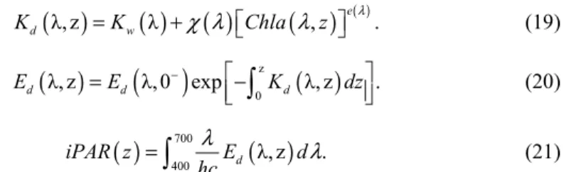
from 400 nm to 700 nm (Eq. 19); Ed profiles are then propagated downward from GC90

surface values (Eq. 20). Finally, the iPAR value is obtained through the integration of spectral Ed from 400nm to 700nm (Eq. 21), where h is Planck's constant and c is the speed of light.

( )

( ) ( )

( )

( )

( )

( )



( )

( )



On the basis of such a modeled iPAR profile, we could compute ziPAR15, and then apply it

to the light-threshold-based correction method (i.e. Eq. 10 to 13), producing two alternative corrected FChla profiles, called as S08m and X12m (‘m’ stands for modeled).

6. Results

Briefly, the model-based S08m and X12m perform better than the original S08 and X12, but do not show clear improvement compared to P18 (even performing worse in w/oDCM-Type, Table 4). The reason is that clear-sky iPAR estimation at surface is higher than the true measurement (figure not shown), which leads to an over-estimation of ziPAR15.

As mentioned above, using the threshold light for NPQ correction is more consistent with the NPQ phenomenon and theory, than using a relative light (i.e. zeu). Therefore, we expect

that such a light-model-based method could be further improved in the future, e.g., by incorporating cloud cover with data from other sources.

Table 4. Statistical results of all correction methods for floats without radiometry.

Correcti on methods

w/oDCM-Type _{Type (z}Deep-mixing

DCM-iPAR15≤ MLD)

Shallow-mixing DCM-Type (ziPAR15 > MLD)

MAE MAPE MPE MAE MAPE MPE MAE MAPE MPE S08 0.072 13.8% 10.0% 0.058 33.9% 26.9% 0.030 34.5% −4.6% X12 0.065 11.5% 6.8% 0.067 35.6% 28.2% 0.031 35.0% −2.8%

P18 0.062 10.6% 4.7% 0.070 35.9% 27.9% *0.031 *35.0% *-2.8% S08m 0.070 13.2% 8.9% 0.057 33.0% 25.9% *0.030 *34.5% *-4.6% X12m 0.064 11.3% 6.2% 0.067 35.0% 27.6% *0.031 *35.0% *-2.8%

* Note that X12m and P18 are identical to X12 and S08m to S08 in shallow-mixing DCM-type.

Funding

Scientific Research Fund of the Second Institute of Oceanography, SOA, China (QNYC1702, 14283); Qingdao National Laboratory for Marine Science and Technology (QNLM2016ORP0103); National Natural Science Foundation of China (41476159, 41730536); Remotely Sensed Biogeochemical Cycles in the Ocean (remOcean) project funded by the European Research Council (GA 246777); ATLANTOS EU project funded by H2020 program (GA 2014-633211); French CNES-TOSCA BGC-Argo program. NASA OBB program (NNX14AP49G); French “Equipement d’avenir” NAOS project (ANR J11R107-F); SOCLIM project funded by the Foundation BNP Paribas; UK Bio-Argo (funded by the Natural Environment Research Council, grant agreement no. NE/L012855/1).

Acknowledgements

These BGC-Argo data were collected and made freely available by the International Argo Program and the national programs that contribute to it: (http://www.argo.ucsd.edu, http://argo.jcommops.org). The Argo Program is part of the Global Ocean Observing System. Discussions with Josh Plant and Ken Johnson (MBARI) have motivated much of this work. Boss thanks Michael Behrenfeld (OSU) for illuminating discussions on the subject of NPQ. Catherine Schmechtig and Antoine Poteau are thanked for their help in managing float missions as well as their crucial role in BGC-Argo data management. We would also like to thank two anonymous reviewers, whose comments substantially improved this paper.