HAL Id: hal-01806682
https://hal.archives-ouvertes.fr/hal-01806682
Submitted on 27 Oct 2020
HAL is a multi-disciplinary open access
archive for the deposit and dissemination of
sci-entific research documents, whether they are
pub-lished or not. The documents may come from
teaching and research institutions in France or
abroad, or from public or private research centers.
L’archive ouverte pluridisciplinaire HAL, est
destinée au dépôt et à la diffusion de documents
scientifiques de niveau recherche, publiés ou non,
émanant des établissements d’enseignement et de
recherche français ou étrangers, des laboratoires
publics ou privés.
emissions based on four different inverse models
P. Bergamaschi, M. Corazza, U. Karstens, M. Athanassiadou, L. Thompson, I.
Pison, A. Manning, P. Bousquet, A. Segers, A. Vermeulen, et al.
To cite this version:
P. Bergamaschi, M. Corazza, U. Karstens, M. Athanassiadou, L. Thompson, et al.. Top-down
es-timates of European CH4 and N2O emissions based on four different inverse models. Atmospheric
Chemistry and Physics, European Geosciences Union, 2015, 15 (2), pp.715 - 736.
�10.5194/acp-15-715-2015�. �hal-01806682�
www.atmos-chem-phys.net/15/715/2015/ doi:10.5194/acp-15-715-2015
© Author(s) 2015. CC Attribution 3.0 License.
Top-down estimates of European CH
4
and N
2
O emissions based on
four different inverse models
P. Bergamaschi1, M. Corazza1,a, U. Karstens2, M. Athanassiadou3, R. L. Thompson4,b, I. Pison4, A. J. Manning3, P. Bousquet4, A. Segers1,c, A. T. Vermeulen5,d, G. Janssens-Maenhout1, M. Schmidt4,e, M. Ramonet4, F. Meinhardt6, T. Aalto7, L. Haszpra8,9, J. Moncrieff10, M. E. Popa2,f, D. Lowry11, M. Steinbacher12, A. Jordan2, S. O’Doherty13, S. Piacentino14, and E. Dlugokencky15
1European Commission Joint Research Centre, Institute for Environment and Sustainability, Ispra, Italy 2Max-Planck-Institute for Biogeochemistry, Jena, Germany
3Met Office, Exeter, UK
4Laboratoire des Sciences du Climat et de l’ Environnement (LSCE), Gif sur Yvette, France 5Energy Research Centre of the Netherlands (ECN), Petten, the Netherlands
6Umweltbundesamt, Messstelle Schauinsland, Kirchzarten, Germany 7Finnish Meteorological Institute (FMI), Helsinki, Finland
8Hungarian Meteorological Service, Budapest, Hungary
9Research Centre for Astronomy and Earth Sciences, Geodetic and Geophysical Institute, Sopron, Hungary 10School of GeoSciences, The University of Edinburgh, Edinburgh, UK
11Dept. of Earth Sciences, Royal Holloway, University of London (RHUL), Egham, UK
12Swiss Federal Laboratories for Materials Science and Technology (Empa), Dübendorf, Switzerland 13Atmospheric Chemistry Research Group, University of Bristol, Bristol, UK
14Italian National Agency for New Technologies, Energy and Sustainable Development (ENEA), Rome, Italy 15NOAA Earth System Research Laboratory, Global Monitoring Division, Boulder, CO, USA
anow at: Agenzia Regionale per la Protezione dell’Ambiente Ligure, Genoa, Italy bnow at: Norwegian Institute for Air Research (NILU), Kjeller, Norway
cnow at: Netherlands Organisation for Applied Scientific Research (TNO), Utrecht,
the Netherlands
dnow at: Dept. of Physical Geography and Ecosystem Science, Lund University, Lund, Sweden enow at: Institut für Umweltphysik, Heidelberg, Germany
fnow at: Institute for Marine and Atmospheric Research Utrecht, Utrecht University, Utrecht, the Netherlands
Correspondence to: P. Bergamaschi ([email protected])
Received: 11 March 2014 – Published in Atmos. Chem. Phys. Discuss.: 16 June 2014 Revised: 12 November 2014 – Accepted: 22 November 2014 – Published: 19 January 2015
Abstract. European CH4 and N2O emissions are estimated
for 2006 and 2007 using four inverse modelling systems, based on different global and regional Eulerian and La-grangian transport models. This ensemble approach is de-signed to provide more realistic estimates of the overall un-certainties in the derived emissions, which is particularly im-portant for verifying bottom-up emission inventories.
We use continuous observations from 10 European sta-tions (including 5 tall towers) for CH4and 9 continuous
sta-tions for N2O, complemented by additional European and
global discrete air sampling sites. The available observa-tions mainly constrain CH4and N2O emissions from
north-western and eastern Europe. The inversions are strongly driven by the observations and the derived total emissions of larger countries show little dependence on the emission inventories used a priori.
Three inverse models yield 26–56 % higher total CH4
to bottom-up emissions reported to the UNFCCC, while one model is close to the UNFCCC values. In contrast, the in-verse modelling estimates of European N2O emissions are in
general close to the UNFCCC values, with the overall range from all models being much smaller than the UNFCCC un-certainty range for most countries. Our analysis suggests that the reported uncertainties for CH4emissions might be
under-estimated, while those for N2O emissions are likely
overes-timated.
1 Introduction
Atmospheric methane (CH4) and nitrous oxide (N2O) are the
second and third most important long-lived anthropogenic greenhouse gases (GHGs), after carbon dioxide (CO2). CH4
and N2O have large global warming potentials of 28 and 265,
respectively, relative to CO2 over a 100-year time horizon
(Myhre et al., 2013). Globally averaged dry-air mole frac-tions of CH4 reached 1819 ± 1 ppb in 2012, 160 % above
the pre-industrial level (1750) of ∼ 700 ppb, while N2O
reached 325.1 ± 0.1 ppb, ∼ 20 % higher than pre-industrial level (270 ppb) (WMO, 2013). CH4 and N2O contributed
∼18 % and ∼ 6 %, respectively, to the direct anthropogenic radiative forcing of all long-lived GHGs in 2012, relative to 1750 (NOAA Annual Greenhouse Gas Index (AGGI), http://www.esrl.noaa.gov/gmd/aggi/). CH4 also has
signifi-cant additional indirect radiative effects due to its feedback on global OH concentrations, tropospheric ozone, and strato-spheric water vapour, and the generation of CO2 as the
fi-nal product of the CH4oxidation chain (Forster et al., 2007;
Shindell et al., 2005). These indirect effects are reflected in the CH4 emission-based radiative forcing of 0.97 (0.74
to 1.20) Wm−2, which is about twice the concentration-based radiative forcing of 0.48 (0.43 to 0.53) Wm−2(Myhre et al., 2013). In addition to its significant contribution to global warming, N2O plays an important role in the
deple-tion of stratospheric ozone, with its current ozone depledeple-tion potential-weighted emissions being the largest of all ozone-depleting substances (Ravishankara et al., 2009).
On the European scale, combined emissions of CH4and
N2O contributed 15.4 % to total GHG emissions (in CO2
-equivalents) reported under the United Nations Framework Convention on Climate Change (UNFCCC) by the EU-15 countries for 2012 (16.3 % for EU-28) (EEA, 2014). The large reductions of both CH4and N2O emissions since 1990
(CH4 by 33 %; N2O by 34 %) reported by the EU-15
con-tributed significantly to the reduction of its total GHG emis-sions by 15.1 % (2012 compared to 1990).
GHG emissions reported to the UNFCCC are based on sta-tistical activity data and source-specific and country-specific emission factors (IPCC, 2006). For CH4and N2O however,
such “bottom-up” emission inventories have considerable uncertainties, mainly due to the large variability of emission
factors, which for many CH4and N2O sources are not very
well characterized (e.g. CH4 emissions from landfills, gas
production facilities and distribution networks, or N2O
emis-sions from agricultural soils (e.g. Karion et al., 2013; Leip et al., 2011)).
Complementarily to “bottom-up” approaches, emissions can be estimated using atmospheric measurements and in-verse modelling. This “top-down” technique is widely used to estimate GHG emissions on the global and continental scale (e.g. Bergamaschi et al., 2013; Bousquet et al., 2006; Hein et al., 1997; Houweling et al., 1999; Kirschke et al., 2013; Mikaloff Fletcher et al., 2004a, b for CH4and Hirsch
et al., 2006; Huang et al., 2008; Thompson et al., 2014 for N2O). With the availability of quasi-continuous GHG
mea-surements and the increasing number of regional monitoring stations, especially in Europe and North America, various inverse modelling studies have estimated emissions also on the regional to country scale (e.g. Bergamaschi et al., 2010; Corazza et al., 2011; Kort et al., 2008; Manning et al., 2011; Miller et al., 2013), demonstrating the potential of using such top-down methods for independent verification of bottom-up inventories (Bergamaschi, 2007). The use of atmospheric measurements and inverse modelling for verification has also been recognized by the IPCC (2006).
Currently, only anthropogenic GHG emissions are re-ported to UNFCCC. In many specific cases, such as the Eu-ropean CH4and N2O emissions discussed in this study, the
contribution of natural emissions is considered to be rela-tively small. Nevertheless, quantitative comparison between inverse modelling and bottom-up estimates also requires es-timates of natural emissions.
A further challenge with inverse modelling, particularly for its use in verifying bottom-up estimates, is the provi-sion of realistic uncertainties for the derived emisprovi-sions. Al-though various studies attempt to take account of estimates of the model representation and transport errors, such esti-mates are typically based on strongly simplified assumptions. As a complementary approach, the range of results from an ensemble of models can be analysed and may be consid-ered a more realistic estimate of the overall uncertainty, pro-vided the applied models are largely independent and repre-sent well the range of current models. Furthermore, detailed model comparisons, and verification with independent vali-dation data, allow the model characteristics to be analysed in detail and potential model deficiencies to be identified. Com-parisons of global inverse models have been performed for CO2 (e.g. Peylin et al., 2013; Stephens et al., 2007), CH4
(Kirschke et al., 2013) and N2O (Thompson et al., 2014),
fo-cusing on the global and continental scale. Here, we present for the first time a detailed comparison of inverse models es-timating European CH4and N2O emissions. We use four
in-verse models, based on different global and regional Eulerian and Lagrangian transport models. The inversions are con-strained by a comprehensive data set of quasi-continuous ob-servations from European monitoring stations (including five
tall towers), complemented by further European and global discrete air sampling sites.
2 Atmospheric measurements
The European monitoring stations used in the CH4and N2O
inversions are summarized in Table 1. The monitoring sta-tions include 10 sites with quasi-continuous measurements for CH4(i.e. providing data with hourly or higher time
res-olution), and 9 sites with quasi-continuous N2O
measure-ments. Five of these stations are equipped with tall tow-ers (Cabauw, Bialystok, Ochsenkopf, Hegyhatsal, and An-gus), with uppermost sampling heights above the surface by 97–300 m. The measurements at the tall towers were set up or improved within the EU project CHIOTTO (“Continuous High-precision Tall Tower Observations”) (Popa et al., 2010; Thompson et al., 2009; Vermeulen et al., 2007, 2011). Addi-tional quasi-continuous measurements are from the AGAGE (Advanced Global Atmospheric Gases Experiment) network (Cunnold et al., 2002; Rigby et al., 2008) at Mace Head, from the operational network of the German Federal Environment Agency (UBA) at Schauinsland, from the Finnish Meteoro-logical Institute at Pallas (Aalto et al., 2007), from the Swiss Federal Laboratories for Materials Science and Technology (EMPA) at Jungfraujoch, and from the Royal Holloway Uni-versity of London (RHUL) in London. Furthermore, we use CH4 and N2O discrete air samples from the NOAA Earth
System Research Laboratory (ESRL) global cooperative air sampling network at 10 European sites (and for the global in-verse models, additional global NOAA sites) (Dlugokencky et al., 1994, 2003, 2009), and CH4discrete air samples from
the French RAMCES (Réseau Atmosphérique de Mesure des Composés à Effet de Serre) network (Schmidt et al., 2006) at 5 European sites. Finally, discrete air samples from the Max-Planck-Institute for Biogeochemistry at the Shetland Islands, and from the Italian National Agency for New Technologies, Energy and Sustainable Development (ENEA) at Lampedusa were used. Both quasi-continuous and discrete air sample measurements are based on gas chromatography (GC) using flame ionization detectors (FIDs) for CH4, and electron
cap-ture detectors (ECDs) for N2O. Measurements are reported
as dry air mole fractions (nmol mol−1, abbreviated as ppb). For CH4, we generally apply the NOAA04 CH4standard
scale (Dlugokencky et al., 2005). AGAGE CH4 data were
converted to NOAA04 using a scaling factor of 1.0003 (Prinn et al., 2000), and RAMCES CH4data were scaled by 1.0124
from CMDL83 to NOAA04 (Dlugokencky et al., 2005). CH4 comparisons of high-pressure cylinders performed in
the frame of the European projects MethMoniteur, IMECC, Geomon and CHIOTTO, and WMO between 2004 and 2010 showed that the CH4measurements of the CHIOTTO,
NOAA, RAMCES, UBA, and RHUL networks agreed within 2 ppb. Furthermore, comparison of the quasi-continuous measurements at Pallas, Mace Head, Ochsenkopf, and
Hegy-hatsal with NOAA discrete air samples (using measurements coinciding within 1 h, and the additional condition that the quasi-continuous measurements show low variability within a 5 h time window) showed annual average absolute CH4
bi-ases of less than 4 ppb during 2006 and 2007, the target pe-riod of this study.
While the merged CH4 data set used in this study can,
therefore, be considered reasonably consistent, this is not the case for N2O, for which significant offsets are apparent
be-tween different monitoring laboratories, even though most laboratories use N2O primary standards from NOAA/ESRL.
These offsets exceed the compatibility goal of ±0.1 ppb (1σ ) recommended by WMO GAW (WMO, 2012) (Table 7). We, therefore, adopt the approach developed by Corazza et al. (2011) to correct for these calibration offsets in the inversion (see also Sect. 3), using the NOAA discrete air samples (which are reported on the NOAA-2006 scale; Hall et al., 2007) as a common reference. Corazza et al. (2011) showed that the N2O bias correction derived in the inversion
agreed within 0.1–0.2 ppb (N2O dry-air mole fraction) with
the bias derived from the comparison of quasi-continuous measurements with parallel NOAA discrete air samples. We emphasize that this bias correction assumes that the bias re-mains constant during the inversion period (yearly for TM5) and, therefore, cannot correct for changes of the systematic bias on shorter timescales.
For validation, CH4measurements of discrete air samples
from three European aircraft profile sites in Scotland, France, and Hungary are used, operated within the European Car-boEurope project. The analyses of these samples were per-formed at LSCE, in the same manner as the RAMCES sur-face measurements.
3 Modelling
3.1 Modelling protocol
The modelling protocol used in this study prescribed mainly the basic settings for the inversions, such as a priori emis-sion inventories, observational data sets, time period, and requested model output. Atmospheric sinks were not pre-scribed. For both CH4and N2O, two types of inversions were
performed: (1) the base inversions, S1–CH4and S1–N2O,
re-spectively, using detailed bottom-up emission inventories for anthropogenic and natural sources as a priori emission esti-mates, and (2) the “free inversions”, S2–CH4and S2–N2O,
which do not use these bottom-up inventories. The objective of these “free inversions” is to explore the information con-tent of the observations in the absence of detailed a priori information.
The CH4 and N2O emission inventories applied in S1–
CH4and S1–N2O are summarized in Tables 3 and 4,
respec-tively. For the anthropogenic sources (except biomass burn-ing), the EDGARv4.1 emission inventory for 2005 was used
Table 1. European atmospheric monitoring stations used in the inversions (2006–2007). “ST” specifies the sampling type (“CM”: quasi-continuous measurements, providing data with hourly time resolution; “FM”: discrete air measurements with typically weekly sampling frequency). “CH4” and “N2O” indicate which stations have been used in the CH4and N2O inversions, respectively.
ID Station name Data provider Latitude Longitude Altitude ST CH4 N2O
m a.s.l.
PAL Pallas, Finland FMI 67.97 24.12 560 CM • •
NOAA FM • •
STM Ocean station M, Norway NOAA 66.00 2.00 5 FM • •
ICE Heimay, Vestmannaeyjar, Iceland NOAA 63.34 −20.29 127 FM • •
SIS Shetland Island, UK MPI-BGC 59.85 −1.27 46 FM • •
TT1 Angus, UK (222 m level) CHIOTTO 56.55 −2.98 535 CM • •
BAL Baltic Sea, Poland NOAA 55.35 17.22 28 FM • •
MHD Mace Head, Ireland AGAGE 53.33 −9.90 25 CM • •
NOAA FM • •
BI5 Bialystok, Poland (300 m level) CHIOTTO 53.23 23.03 460 CM • •
CB3 Cabauw, Netherlands (120 m level) CHIOTTO 51.97 4.93 118 CM • •
LON Royal Holloway, London, UK RHUL 51.43 −0.56 45 CM •
OX3 Ochsenkopf, Germany (163 m level) CHIOTTO 50.05 11.82 1185 CM • •
NOAA FM • •
LPO Ile Grande, France RAMCES 48.80 −3.58 30 FM •
GIF Gif sur Yvette, France RAMCES 48.71 2.15 167 FM •
SIL Schauinsland, Germany UBA 47.91 7.91 1205 CM • •
HPB Hohenpeissenberg, Germany NOAA 47.80 11.01 985 FM • •
HU1 Hegyhatsal, Hungary (96 m level) CHIOTTO 46.95 16.65 344 CM • •
NOAA FM • •
JFJ Jungfraujoch, Switzerland EMPA 46.55 7.98 3580 CM • •
PUY Puy de Dome, France RAMCES 45.77 2.97 1475 FM •
BSC Black Sea, Constanta, Romania NOAA 44.17 28.68 3 FM • •
PDM Pic du Midi, France RAMCES 42.94 0.14 2887 FM •
BGU Begur, Spain RAMCES 41.97 3.23 15 FM •
LMP Lampedusa, Italy ENEA 35.52 12.63 45 FM •
NOAA FM •
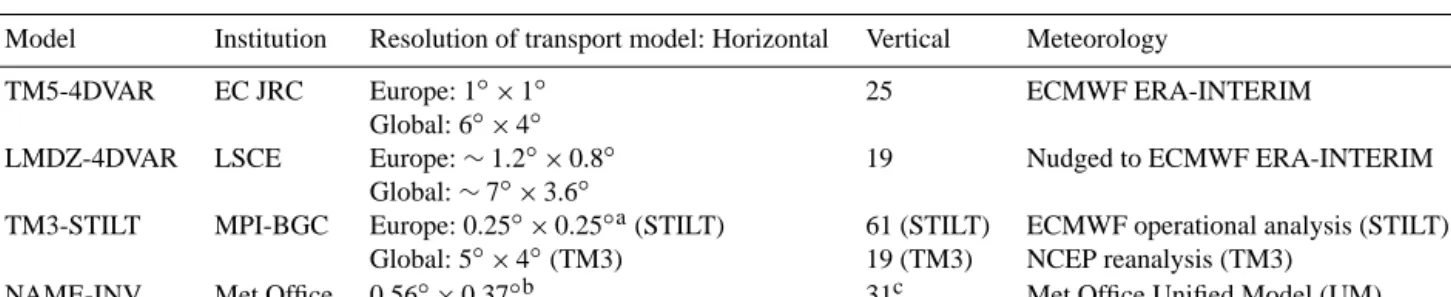
Table 2. Atmospheric models.
Model Institution Resolution of transport model: Horizontal Vertical Meteorology
TM5-4DVAR EC JRC Europe: 1◦×1◦ 25 ECMWF ERA-INTERIM Global: 6◦×4◦
LMDZ-4DVAR LSCE Europe: ∼ 1.2◦×0.8◦ 19 Nudged to ECMWF ERA-INTERIM Global: ∼ 7◦×3.6◦
TM3-STILT MPI-BGC Europe: 0.25◦×0.25◦a(STILT) 61 (STILT) ECMWF operational analysis (STILT) Global: 5◦×4◦(TM3) 19 (TM3) NCEP reanalysis (TM3)
NAME-INV Met Office 0.56◦×0.37◦b 31c Met Office Unified Model (UM)
aHorizontal resolution of inversion: 1◦×1◦. bHorizontal resolution of inversion: 0.42◦×0.27◦. c31 levels from surface to 19 km.
(as 2005 is the most recent available year in EDGARv4.1). For S2–CH4 and S2–N2O, a homogeneous distribution of
emissions over land and over the ocean was used as starting point for the optimization (i.e. a “weak a priori” for TM5-4DVAR and TM3-STILT), with global total CH4 and N2O
emissions over land and over the ocean, respectively, close to the total emissions over land and over the ocean of the de-tailed a priori inventories (Bergamaschi et al., 2010; Corazza
et al., 2011), hence effectively limiting the emissions that can be attributed to the ocean. For the NAME-INV model, no separation was made between land and ocean. Moreover, the NAME-INV model started from random emission maps rather than a homogeneous distribution of emissions. Inver-sions S2 were not available for LMDZ-4DVAR.
For the European limited domain models NAME-INV and STILT, background CH4and N2O mixing ratios were
calcu-Table 3. CH4emission inventories used as a priori in inversion S1–CH4.
Source Inventory Global total
Tg CH4yr−1
Anthropogenic
Coal mining EDGARv4.1a 40.3
Oil production and refineries EDGARv4.1a 26.1 Gas production and distribution EDGARv4.1a 46.8 Enteric fermentation EDGARv4.1a 96.9 Manure management EDGARv4.1a 11.3 Rice cultivation EDGARv4.1a 34.0
Solid waste EDGARv4.1a 28.1
Waste water EDGARv4.1a 30.0
Further anthropogenic sourcesb EDGARv4.1a 16.9 Biomass burning GFEDv2 (van der Werf et al., 2004) 19.7–20.2c Natural
Wetlands Inventory of J. Kaplan (Bergamaschi et al., 2007) 175.0 Wild animals (Houweling et al., 1999) 5.0 Termites (Sanderson, 1996) 19.3 Ocean (Lambert and Schmidt, 1993) 17.0 Soil sink (Ridgwell et al., 1999) −37.9
Total 528.4–528.9d
aEDGARv4.1 CH
4emissions for 2005. bIncluding CH
4emission from transport, residential sector, energy manufacturing and transformation, industrial processes and product use, and agricultural waste burning.
cGFEDv2 CH
4emissions for 2006 and 2007, respectively. dGlobal total CH
4emissions for 2006 and 2007, respectively.
Table 4. N2O emission inventories used as a priori in inversion S1–N2O.
Source Inventory Global total Tg N2O yr−1
anthropogenic
Agricultural soils EDGARv4.1a 4.5 Indirect N2O emissions EDGARv4.1a 1.6
Manure management EDGARv4.1a 0.3
Transport EDGARv4.1a 0.3
Residential EDGARv4.1a 0.3
Industrial processes and product use EDGARv4.1a 0.6 Energy manufacturing and transformation EDGARv4.1a 0.3
Waste EDGARv4.1a 0.4
Further anthropogenic sourcesb EDGARv4.1a 0.1 Biomass burning GFEDv2 (van der Werf et al., 2004) 1.0–1.1c Post-forest clearing enhanced (Bouwman et al., 1995) 0.6 Natural
Natural soils (Bouwman et al., 1995) 7.2 Ocean (Bouwman et al., 1995) 5.7
Total 22.7–22.8d
aEDGARv4.1 N
2Oemissions for 2005. bIncluding N
2Oemission from agricultural waste burning, and oil and gas sector. cGFEDv2 N
2Oemissions for 2006 and 2007, respectively. dGlobal total N
lated by TM5-4DVAR (for NAME-INV CH4and N2O
inver-sions and STILT N2O inversions) and by TM3 (for STILT
CH4 inversions) following the two-step scheme of
Röden-beck et al. (2009).
All models used the same observational data set described in Sect. 2 (with the exception of a few stations that are out-side the domain of the limited domain models). For the con-tinuously operated monitoring stations in the boundary layer, measurements between 12:00 and 15:00 LT were assimilated, when measurements (and model simulations) are usually rep-resentative of large regions and much less affected by local emissions. In contrast, for mountain sites night-time mea-surements (between 00:00 and 03:00 LT) were used to avoid the potential influence of upslope transport on the measure-ments, which is frequently observed at mountain stations during daytime. Different from this sampling scheme (ap-plied in TM5-4DVAR, LMDZ-4DVAR, and TM3-STILT), the NAME-INV model used observations at all times, but with local contributions excluded as in Manning et al. (2011). For the N2O inversions, bias corrections for the N2O
ob-servations from different networks or institutes were calcu-lated within the 4DVAR optimization of the TM5-4DVAR and LMDZ-4DVAR models, as described by Corazza et al. (2011). For NAME-INV and TM3-STILT, the bias cor-rections calculated by TM5-4DVAR (Table 7) were applied.
3.2 Atmospheric models
The atmospheric models used in this study are summarized in Table 2 and briefly described in the following.
3.2.1 TM5-4DVAR
The TM5-4DVAR inverse modelling system is described in detail by Meirink et al. (2008). It is based on the two-way nested atmospheric zoom model TM5 (Krol et al., 2005). In this study we apply the zooming with 1◦×1◦resolution over Europe, while the global domain is simulated at a hor-izontal resolution of 6◦(longitude) × 4◦ (latitude). TM5 is an offline transport model, driven by meteorological fields from the European Centre for Medium-Range Weather Fore-casts (ECMWF) ERA-Interim reanalysis (Dee et al., 2011). The 4-dimensional variational (4DVAR) optimization tech-nique minimizes iteratively a cost function using the adjoint of the tangent linear model and the m1qn3 algorithm for min-imization (Gilbert and Lemaréchal, 1989). We apply a “semi-exponential” description of the probability density function for the a priori emissions to force the a posteriori emissions to remain positive (Bergamaschi et al., 2009, 2010). In inver-sion S1–CH4, four groups of CH4 emissions are optimized
independently: (1) wetlands, (2) rice, (3) biomass burning, and (4) all remaining sources (Bergamaschi et al., 2010). For S1–N2O the following four groups of N2O emissions
are optimized: (1) soil, (2) ocean, (3) biomass burning, and (4) all remaining emissions (Corazza et al., 2011). In S2–
CH4 and S2–N2O, only total emissions are optimized. We
assume uncertainties of 100 % per grid-cell and month for each source group and apply spatial correlation scale lengths of 200 km in S1–CH4and S1–N2O. In the “free inversions”
S2–CH4 and S2–N2O, smaller correlation scale lengths of
50 km, and larger uncertainties of 500 % per grid-cell and month are used to give the inversion enough freedom to re-trieve regional hot spots (Bergamaschi et al., 2010; Corazza et al., 2011). The temporal correlation timescales are set to zero for the source groups with significant seasonal varia-tions, and 9.5 months for the “remaining” CH4 and N2O
sources (which include major anthropogenic sources that are assumed to have no or only small seasonal variations) in S1– CH4and S1–N2O, and 1 month for the total emissions
opti-mized in S2–CH4and S2–N2O.
The photochemical sinks of CH4(due to OH in the
tropo-sphere, and OH, Cl, and O(1D) in the stratosphere) are sim-ulated as described in Bergamaschi et al. (2010). The strato-spheric sinks of N2O (photolysis and reaction with excited
oxygen O(1D)) are modelled as in Corazza et al. (2011). The observation errors were set to 3 ppb for CH4, and
0.3 ppb for N2O. The model representation error is estimated
as a function of local emissions and 3-D gradients of simu-lated mixing ratios (Bergamaschi et al., 2010), resulting in overall (combined measurement and model representation) errors in the range between 3 ppb and up to ∼ 1 ppm for CH4,
and between 0.3 ppb and up to several ppb for N2O. For the
N2O inversions we optimize bias parameters for the N2O
ob-servations from different networks or institutes (see Table 7), as described by Corazza et al. (2011).
3.2.2 LMDZ-4DVAR
The LMDZ-4DVAR inverse modelling framework is based on the offline and adjoint models of the Laboratoire de Météorologie Dynamique, version 4 (LMDZ) general cir-culation model (Hourdin and Armengaud, 1999; Hourdin et al., 2006). The offline model is driven by archived fields of winds, convection mass fluxes, and planetary boundary layer (PBL) exchange coefficients that have been calculated in prior integrations of the complete general circulation model, which was nudged to ECMWF ERA-Interim winds (Dee et al., 2011). In this study, LMDZ is used with a zoom over Europe at a resolution of approximately 1.2◦×0.8◦and de-creasing resolution away from Europe to a maximum grid size of approximately 7.2◦×3.6◦. LMDZ has 19 hybrid pres-sure levels in the vertical dimension. The optimal fluxes were found by solving the cost function using the adjoint model and the Lanczos algorithm for N2O and the m1qn3 algorithm
for CH4.
Details about the inversion framework for CH4 are given
in Pison et al. (2009, 2013). Only the total net emissions of methane are optimized, at the resolution of the grid-cell for 8-day periods. Prior uncertainties in each grid-cell are set to 100 % of the maximum flux over the grid-cell and its
eight neighbours (so as to allow for a misplacement of the sources). Correlation scale lengths are used to compute the off-diagonal terms in the error covariance matrix: they are set at 500 km on land and 1000 km on sea (land and sea are not correlated); there are no time correlations. The “observation” errors include the estimates of the errors due to the transport model and to the representativity of the grid-cell compared to the measurement (combined measurement and model er-ror ranging between 3 ppb and up to 450 ppb). Note that the OH fields are inverted simultaneously to the methane emis-sions, with constraints from methyl-chloroform (Pison et al., 2009; 2013).
Details about the inversion framework for N2O can be
found in Thompson et al. (2011). For N2O, only total
emis-sions were optimized. Prior uncertainties in each grid-cell were set to 100 % and correlation scale lengths of 500 km over land, 1000 km over ocean, and 3 months were used to form the full error covariance matrix, which was subse-quently scaled to be consistent with a global total uncertainty of 3 TgN yr−1(approximately 18 %). The error of the N2O
observations was set to 0.3 ppb. Model representation errors incorporated an estimate of aggregation error, i.e. distribution of emissions within the grid-cell (Bergamaschi et al., 2010), and horizontal advection errors (Rödenbeck et al., 2003), re-sulting in total model errors ranging from about 0.2 ppb to 1 ppb. In addition to the emissions, bias parameters for the N2O observations from different networks or institutes were
optimized, similarly to TM5-4DVAR (Corazza et al., 2011).
3.2.3 TM3-STILT
In the Jena inversions, the coupled system TM3-STILT is used for regional-scale high-resolution inversions. TM3-STILT (Trusilova et al., 2010) is a combination of the coarse-grid global 3-dimensional atmospheric offline trans-port model TM3 (Heimann and Koerner, 2003) and the fine-scale regional Stochastic Time-Inverted Lagrangian Trans-port model STILT (Gerbig et al., 2003; Lin et al., 2003). The models are coupled using the two-step nesting scheme of Rö-denbeck et al. (2009), which allows the use of completely independent models for the representation of the global and the regional transport. The variational inversion algorithm of the Jena inversion scheme, applied in the global as well as in the regional inversion step, is described in detail in Röden-beck (2005). In this study, the global transport model TM3 is used with a spatial resolution of 4◦×5◦and 19 vertical
lev-els. STILT is driven by meteorological fields from ECMWF operational analysis, used here with a spatial resolution of 0.25◦×0.25◦and confined to the lowest 61 vertical layers. The regional TM3-STILT inversions are conducted in this study on a 1◦×1◦ horizontal resolution grid covering the greater part of Europe (12◦W–35◦E, 35–62◦N). Regional inversion results for CH4were obtained directly by the
TM3-STILT system. For the regional N2O inversions the same
modular nesting technique is applied to couple STILT with
a baseline provided by TM5-4DVAR (Bergamaschi et al., 2010; Corazza et al., 2011) and the regional inversion step is performed in the Jena inversion system. The latter com-bination is referred to as TM5-STILT in the presentation of the N2O inversion results. In all regional inversions we
opti-mize the total emissions. Uncertainties of 100 % per grid-cell and month, with a spatial correlation scale length of 600 km and a temporal correlation timescale of 1 month, are assumed in the regional S1–CH4and S1–N2O inversions. In both S2
inversions the uncertainties are set to 500 % with a corre-lation scale length of 60 km and correcorre-lation timescale of 1 month. The observation errors were set to 3 ppb for CH4and
0.2 ppb for N2O. Model representation errors are assigned to
the individual sites according to their location with respect to continental, remote or oceanic situations (Rödenbeck, 2005), resulting in overall (combined measurement and model rep-resentation) errors in the range of 10–30 ppb for CH4, and 0.8
and 2.4 ppb for N2O. For N2O the bias parameters estimated
by TM5-4DVAR (see Table 7) are applied in the regional in-versions.
3.2.4 NAME-INV
The NAME-INV inverse modelling system is described in Manning et al. (2011) using one station to estimate UK and Northern European emissions of various trace gases and in Athanassiadou et al. (2011) for multiple stations across Eu-rope. The transport of CH4and N2O from sources to
obser-vations is performed using the UK Met Office Lagrangian model NAME (Jones et al., 2007). Thousands of particles are released from each measurement for each 2 h period in 2006 and 2007, and these are tracked backwards in time over a period of 13 days (long enough for the majority of particles to leave the domain of interest). The 13-day time-integrated concentrations only include contributions from 0 to 100 m a.g.l., representative of surface emissions. The me-teorological fields needed to run NAME are from the global version of the Met Office Unified Model (UM) at a resolu-tion of 0.56◦×0.37◦ and 31 vertical levels from surface to about 19 km (see Table 2). The domain used for the inver-sion extends from 14.63◦W to 39.13◦E and from 33.81◦N to 72.69◦N, with a resolution of 0.42◦×0.27◦in the longi-tudinal and latilongi-tudinal directions respectively. The inversion is initialized either from the modelling protocol a priori or from a random emissions field as in Manning et al. (2011). In the latter case, the cost function used in the optimization is the same as in Manning et al. (2011). In S1, when the inver-sion is initialized and guided by the a priori emisinver-sion inven-tory, a modified version is used (original cost function + root mean square error (RMSE) between modelled values and a priori). To account for the imbalance in the contribution from different grid boxes (i.e. the grids more distant from the observations are expected to contribute less than those that are closer), grid boxes are progressively grouped together
into increasingly larger boxes as the individual contributions decrease.
In all inversions, the total annual emissions are optimized without any partitioning to various sectors. The background values used for CH4and N2O are from TM5-4DVAR
follow-ing the two-step scheme of Rödenbeck et al. (2009). Obser-vations at all times have been used (i.e. not only in the time windows specified in Sect. 3.1), but excluding local contribu-tions (Manning et al., 2011). An estimate of the uncertainty in the emissions is obtained from the 5th and 95th percentiles of 52 independent inversion solutions (the mean of these be-ing the final solution). The independent inversion solutions are considered to simulate uncertainties in the meteorology, dispersion and observations. For each inversion a different time series of random noise is applied to the observations. The random element at each observation is multiplicative and taken from a lognormal distribution with mean 1 and vari-ance, arbitrarily, set to one fifth of the standard deviation of baseline observations about a smoothed baseline value as in Manning et al. (2011). For this project the baseline standard deviation values 9.5 ppb (CH4) and 0.194 ppb (N2O) were
used.
4 Results and discussion
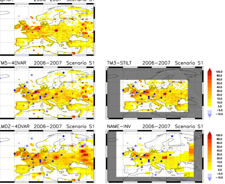
4.1 Inverse modelling of European CH4emissions Figures 1 and 2 show maps of derived CH4emissions
(av-erage 2006–2007) for inversions S1–CH4and S2–CH4,
re-spectively. Guided by the a priori emission inventory in in-version S1–CH4, TM5-4DVAR, TM3-STILT and
LMDZ-4DVAR largely preserve the “fine structure” of the a priori spatial patterns, but calculate some moderate emission in-crements on larger regional scales (determined by the cho-sen spatial correlation scale lengths, ranging between 200 and 600 km). Larger emission increments are apparent for inversion S1–CH4of NAME-INV, with generally lower CH4
emissions across Europe, compared to the a priori and the a posteriori emissions of the other three models.
Inversion S2–CH4, which is not constrained by a detailed
a priori emission inventory, shows in general a smoother spatial distribution than S1–CH4. While the NAME-INV
model does not use any a priori information in S2–CH4,
TM5-4DVAR and TM3-STILT assume that CH4 emissions
are mainly over land. Consequently, NAME-INV attributes much larger emissions over the sea than TM5-4DVAR and TM3-STILT, especially over the North Sea and the Bay of Biscay. All three models show consistently high CH4
emis-sions over the Benelux countries and north-western Ger-many (especially over the highly populated and industrial-ized Ruhr area). Apart from these hotspot emission areas, TM5-4DVAR and TM3-STILT overall show relatively sim-ilar distributions over land, while the NAME-INV inver-sion differs significantly, for example, over Spain and
south-eastern France / north-western Italy, where NAME-INV at-tributes much lower emissions compared to TM5-4DVAR and TM3-STILT.
It is interesting to compare the inversions S2–CH4 and
the a priori used for S1–CH4, representing completely
in-dependent emission estimates, top-down and bottom-up re-spectively. Both approaches show coherently elevated CH4
emissions over Benelux/north-western Germany, and south-ern UK. The S2–CH4 inversions also show somewhat
el-evated emissions per area in southern Poland, where large coal mines are located. However, the inversions are not able to reproduce the very pronounced CH4 emission hotspot
of the bottom-up inventory in this area. This is proba-bly largely due to the limitations of the inversion’s ability to resolve point sources accurately (also given the limita-tion of the sparse atmospheric measurement network) but could also point to a bottom-up overestimate of the CH4
emissions from the coal mining in this area. In fact, the EDGARv4.2 estimate of CH4 emissions from coal mines
in Poland (1.71 Tg CH4yr−1) is about 4 times higher than
that reported under UNFCCC (0.43 Tg CH4yr−1; see
Ta-ble 6). However, it should be pointed out that the bottom-up emissions have large uncertainties, estimated to be 49 % for UNFCCC, and 83 % for EDGARv4.2 for the coal mines in Poland.
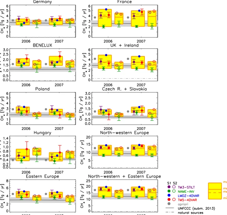
In the following discussion, we analyse the CH4emissions
per country for the countries whose emissions are reason-ably well constrained by the available observations. These are mainly north-western and eastern European countries (Fig. 3), while southern European countries are poorly con-strained. For smaller countries, we present aggregated emis-sions (e.g. Benelux), as they are considered more robust than emissions of individual small countries. The normal-ized range of derived CH4 emissions (defined as (Emax−
Emin)/(Emax+Emin)) is between ±16 and ±44 % for the
analysed countries (or combined countries), and ±25 % for the total CH4emissions of all north-western and eastern
Eu-ropean countries shown in Fig. 3 (inversion S1–CH4). For
some countries, the range of emission estimates from all four models is close to the uncertainties estimated for the individ-ual inversions (e.g. Poland), but there are also several coun-tries with much larger emission ranges (e.g. France). This shows that there are systematic differences between the in-versions, which are not covered by the uncertainty estimates of the individual inversions.
The country totals of the “free” inversion S2–CH4are in
general very close to those of S1–CH4 for most countries,
demonstrating the strong observational constraints. Appar-ently, the above-mentioned differences in the smaller-scale “fine structure” in the spatial patterns between S1–CH4and
S2–CH4(see Figs. 1 and 2) are largely compensated by
ag-gregating emissions on the country scale. The fact that in sev-eral cases the emission ranges of the S2–CH4inversions are
smaller than for S1–CH4 is probably mainly due to fewer
Figure 1. European CH4emissions (average 2006–2007, inversion S1–CH4). Filled circles are measurement stations with quasi-continuous
measurements; open circles are discrete air sampling sites. Table 5. CH4and N2O inversions summary.
Inversion A priori emission inventory TM5-4DVAR LMDZ-4DVAR TM3-STILT NAME-INV CH4inversions S1–CH4 As compiled in Table 3 • • • • S2–CH4 No a priori • • • N2O inversion S1–N2O As compiled in Table 4 • • • • S2–N2O No a priori • • •
For most countries, the NAME-INV model yields lower emissions compared to the other three models. This is most clearly visible in the total emission of all north-western and eastern European countries, which NAME-INV estimates to be 10.7–11.7 Tg CH4yr−1(annual totals for 2006 and 2007,
for S1–CH4 and S2–CH4), compared to estimates of 16.0–
19.4 Tg CH4yr−1 from TM5-4DVAR, LMDZ-4DVAR and
TM3-STILT.
The reasons for the generally lower emissions derived by NAME-INV remain unclear. One factor that may contribute
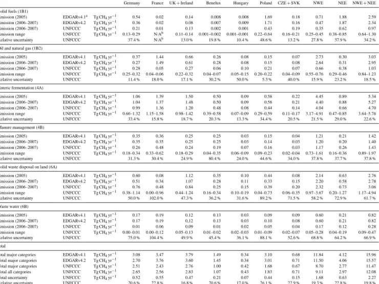
Table 6. CH4emissions from EDGARv4.1, EDGARv4.2, and UNFCCC for major CH4source categories. For the UNFCCC emissions, the reported relative uncertainties (2σ ) per country and category and corresponding emission ranges are also compiled. Total uncertainties per country (or aggregated countries) are estimated from the reported uncertainties per category assuming no correlation between different UNFCCC categories (but correlated errors for sub-categories). “NWE” is the total of the north-western European countries Germany, France, UK, Ireland and Benelux. “NEE” is the total of the eastern European countries Hungary, Poland, Czech Republic (CZE) and Slovakia (SVK).
Germany France UK + Ireland Benelux Hungary Poland CZE + SVK NWE NEE NWE + NEE Solid fuels (1B1) Emission (2005) EDGARv4.1a Tg CH 4yr−1 0.54 0.02 0.14 0.008 0.008 1.69 0.18 0.71 1.88 2.59 Emission (2006–2007) EDGARv4.2 Tg CH4yr−1 0.36 0.02 0.08 0.007 0.009 1.71 0.16 0.47 1.87 2.34 Emission (2006–2007) UNFCCC Tg CH4yr−1 0.21 0.01 0.13 0.002 0.001 0.43 0.19 0.35 0.62 0.97
Emission range UNFCCC Tg CH4yr−1 0.13–0.29 N/Ab 0.11–0.14 0.001–0.002 0.001–0.001 0.22–0.64 0.16–0.21 0.25–0.45 0.38–0.85 0.64–1.30
Relative uncertainty UNFCCC 37.4 % N/Ab 13.0 % 19.8 % 10.4 % 48.6 % 13.2 % 27.8 % 37.9 % 34.2 %
Oil and natural gas (1B2)
Emission (2005) EDGARv4.1 Tg CH4yr−1
0.37 1.44 0.66 0.26 0.08 0.15 0.07 2.73 0.30 3.03 Emission (2006–2007) EDGARv4.2 Tg CH4yr−1 0.27 1.49 0.61 0.28 0.08 0.15 0.08 2.64 0.31 2.95
Emission (2006–2007) UNFCCC Tg CH4yr−1 0.28 0.05 0.27 0.06 0.10 0.21 0.07 0.66 0.38 1.03
Emission range UNFCCC Tg CH4yr−1 0.25–0.32 0.04–0.06 0.22–0.32 0.04–0.07 0.05–0.15 0.20–0.22 0.04–0.09 0.55–0.76 0.29–0.46 0.84–1.23
Relative uncertainty UNFCCC 11.4 % 18.0 % 17.1 % 30.2 % 50.0 % 5.3 % 40.0 % 15.9 % 23.2 % 18.5 % Enteric fermentation (4A)
Emission (2005) EDGARv4.1 Tg CH4yr−1
1.06 1.39 1.50 0.50 0.09 0.58 0.22 4.45 0.89 5.34 Emission (2006–2007) EDGARv4.2 Tg CH4yr−1 1.04 1.37 1.48 0.50 0.09 0.58 0.21 4.40 0.88 5.27
Emission (2006–2007) UNFCCC Tg CH4yr−1 0.99 1.36 1.20 0.48 0.08 0.44 0.14 4.04 0.66 4.70
Emission range UNFCCC Tg CH4yr−1 0.66–1.32 1.15–1.58 0.98–1.42 0.39–0.58 0.07–0.09 0.29–0.59 0.11–0.17 3.17–4.91 0.47–0.85 3.64–5.76
Relative uncertainty UNFCCC 33.4 % 15.8 % 18.7 % 20.3 % 13.3 % 34.4 % 20.5 % 21.5 % 29.0 % 22.6 % Manure management (4B)
Emission (2005) EDGARv4.1 Tg CH4yr−1 0.35 0.36 0.25 0.25 0.03 0.15 0.04 1.21 0.21 1.42
Emission (2006–2007) EDGARv4.2 Tg CH4yr−1
0.35 0.35 0.25 0.25 0.03 0.14 0.03 1.20 0.20 1.40 Emission (2006–2007) UNFCCC Tg CH4yr−1 0.26 0.48 0.24 0.19 0.07 0.16 0.03 1.17 0.26 1.43
Emission range UNFCCC Tg CH4yr−1 0.18–0.34 0.33–0.62 0.18–0.29 0.04–0.35 0.06–0.09 0.09–0.23 0.02–0.04 0.73–1.61 0.16–0.36 0.89–1.97
Relative uncertainty UNFCCC 31.3 % 30.4 % 24.9 % 80.4 % 24.0 % 44.6 % 34.0 % 37.8 % 37.7 % 37.8 % Solid waste disposal on land (6A)
Emission (2005) EDGARv4.1 Tg CH4yr−1 0.60 0.08 1.12 0.35 0.10 0.44 0.08 2.14 0.63 2.76
Emission (2006–2007) EDGARv4.2 Tg CH4yr−1 0.51 0.34 1.07 0.28 0.11 0.33 0.15 2.20 0.58 2.78
Emission (2006–2007) UNFCCC Tg CH4yr−1
0.76 0.48 0.84 0.25 0.15 0.39 0.20 2.32 0.73 3.06 Emission range UNFCCC Tg CH4yr−1 0.38–1.14 0.00–0.96 0.44–1.24 0.16–0.34 0.10–0.19 0.04–0.73 0.06–0.35 0.97–3.67 0.20–1.27 1.17–4.94
Relative uncertainty UNFCCC 50.0 % 102.0 % 47.3 % 36.2 % 31.6 % 89.2 % 71.5 % 58.2 % 72.9 % 61.7 % Waste water (6B)
Emission (2005) EDGARv4.1 Tg CH4yr−1 0.17 0.19 0.12 0.13 0.03 0.09 0.09 0.60 0.21 0.82
Emission (2006–2007) EDGARv4.2 Tg CH4yr−1 0.17 0.19 0,12 0.13 0.03 0.10 0.08 0.60 0.21 0.82
Emission (2006–2007) UNFCCC Tg CH4yr−1 0.01 0.06 0.09 0.01 0.02 0.05 0.04 0.17 0.12 0.28
Emission range UNFCCC Tg CH4yr−1 0.00–0.01 0.00–0.12 0.05–0.13 0.01–0.02 0.02–0.03 0.01–0.09 0.02–0.07 0.05–0.28 0.04–0.19 0.09–0.47 Relative uncertainty UNFCCC 75.0 % 104.4 % 49.9 % 45.4 % 36.1 % 88.1 % 52.6 % 68.8 % 64.2 % 66.9 % total
total major categories EDGARv4.1 Tg CH4yr−1 3.08 3.47 3.79 1.49 0.34 3.10 0.68 11.84 4.12 15.96
Total major categories EDGARv4.2 Tg CH4yr−1 2.70 3.76 3.60 1.45 0.34 3.01 0.71 11.50 4.06 15.57
Total major categories UNFCCC Tg CH4yr−1 2.51 2.43 2.76 1.00 0.42 1.68 0.67 8.70 2.77 11.47
Total all categories UNFCCC Tg CH4yr−1
2.65 2.56 2.83 1.07 0.43 1.83 0.71 9.11 2.97 12.08 Total uncertainty UNFCCC Tg CH4yr−1 0.52 0.55 0.47 0.21 0.07 0.44 0.15 1.68 0.63 2.27
Relative uncertainty UNFCCC 20.6 % 22.8 % 16.8 % 20.6 % 17.0 % 26.1 % 22.9 % 19.3 % 22.8 % 19.8 %
aRecovery from coal mines not included in EDGARv4.1.bUncertainty of CH4emissions from solid fuels in France not available.
is the use of different meteorology in NAME-INV (i.e. me-teorology from the Met Office UM) and the other three mod-els (using ECMWF meteorology, albeit different production streams). In sensitivity experiments Manning et al. (2011) found differences of ∼ 10–20 % (with different signs for dif-ferent years) in derived emissions from the UK and north-western Europe, when using ECMWF ERA-Interim instead of Met Office UM meteorology. Hence, differences in the applied meteorological data sets can have a significant im-pact, but probably explain only part of the differences be-tween NAME-INV and the other models.
In the case of S2–CH4, the difference in the CH4
emis-sions attributed to European countries could be partly due to the higher emissions allocated by NAME-INV to the sea (Figs. 2 and 4). In the absence of any a priori constraint, NAME-INV allocates 4.5–4.9 Tg CH4yr−1 over the
Euro-pean seas (of which ∼ 1 Tg CH4yr−1 over the North Sea),
while sea emissions are largely suppressed in TM5-4DVAR and TM3-STILT in S2–CH4(< 0.2 Tg CH4yr−1over the
Eu-ropean seas). In the case of S1–CH4, the range of CH4
emis-sions attributed to the sea by the different models is gener-ally much smaller, 0.6–2.2 Tg CH4yr−1, due to a priori
con-straints.
In this study we use the same country mask (from EDGAR) for all models to enable a consistent comparison among all models. This country mask accounts only for emis-sions over land (in the case of coastal grid-cells, the total emissions of this grid-cell are attributed to the land). In con-trast, previous NAME-INV inversion studies used different country masks, taking into account also offshore emissions at some further distance from the coastlines (Manning et al., 2011).
Figure 2. European CH4emissions (average 2006–2007, inversion S2–CH4). Filled circles are measurement stations with quasi-continuous
measurements; open circles are discrete air sampling sites.
Table 7. Bias of quasi-continuous N2O measurements. “CM-FM” denotes the annual average bias between quasi-continuous N2O
measure-ments and NOAA discrete air samples (using measuremeasure-ments coinciding within 1 h, and the additional condition that the quasi-continuous measurements show low variability (max 0.3 ppb) within a 5 h time window; mean ± 1 σ in units of ppb; n: number of coinciding mea-surements). The columns “TM5–4DVAR” and “ LMDZ-4DVAR” give the bias corrections (vs. NOAA flask samples) calculated by the models for inversion S1 (for TM5-4DVAR calculated separately for 2006 and 2007, while LMDZ-4DVAR calculated the average bias over 2006–2007).
Station CM-FM TM5-4DVAR CM-FM TM5-4DVAR LMDZ-4DVAR 2006 2006 2007 2007 2006–2007 PAL 0.50 ± 0.33 (n = 32) 0.46 0.31 ± 0.40 (n = 40) 0.26 0.53 SIS 0.51 0.64 0.66 TT1 0.86 1.04 0.91 MHD 0.09 ± 0.29 (n = 28) −0.06 0.35 ± 0.53 (n = 31) 0.06 0.13 BI5 0.27 0.21 0.19 CB3 0.31 0.59 0.70 OX3 1.07 (n = 1) 1.29 0.73 ± 0.21 (n = 3) 1.23 1.35 SIL 0.48 0.17 0.54 HU1 0.37 ± 0.83 (n = 12) 0.38 0.58 (n = 1) 0.39 0.26 JFJ −0.41 −0.23 −0.26
It is important to note that the inverse modelling estimates the total of the anthropogenic and natural emissions. Accord-ing to the bottom-up inventories applied in our study, how-ever, it is estimated that natural CH4 emissions play only
a minor role for the countries considered here (shown by the dashed/dotted lines in Figs. 3 and 4). This is important when comparing the CH4emissions derived by the inverse models
with anthropogenic CH4emissions reported to the UNFCCC
(shown by black lines in Fig. 3). The range of CH4emissions
estimated by the inverse models overlaps for most coun-tries with the uncertainty range of the UNFCCC emissions. Nevertheless, there is a clear tendency to higher CH4
emis-sions derived by three of the inverse models (TM5-4DVAR, LMDZ-4DVAR, TM3-STILT) compared to UNFCCC, while NAME-INV is in most cases close to UNFCCC. For compar-ing different approaches, realistic uncertainty estimates are
726 P. Bergamaschi et al.: Top-down estimates of European CH4and N2O emissions
Figure 3. European CH4emissions by country and aggregated region. For each year, the left yellow box shows the results for inversion S1–
CH4, and the right yellow box for S2–CH4. The grey-shaded area is the range of UNFCCC CH4emissions (based on reported uncertainties,
as compiled in Table 6).
Figure 3. European
CH
4emissions by country and aggregated region. For each year, the left yellow box shows the results for inversion S1–
CH
4, and the yellow right box for S2–CH
4. The grey-shaded area is the range of UNFCCC
CH
4emissions (based on reported uncertainties,
as compiled in Table 6).
Figure 4.
CH
4emissions over European seas. Left: total
CH
4emissions between 35
◦and 62
◦N, and 12
◦W and 35
◦E, representing the
Figure 4. CH4emissions over European seas. Left: total CH4emissions between 35◦and 62◦N, and 12◦W and 35◦E, representing the
P. Bergamaschi et al.: Top-down estimates of European CH4and N2O emissions 727
Figure 5. Comparison of modeled and observedCH4at stations: correlation coefficients (top) and root mean square (RMS) differences
(bottom) for inversion S1–CH4. “All” denotes the mean correlation coefficient and RMS difference, averaged over those stations, for which
results were available from all models.
Figure 6. GEOMON aircraft profile measurements ofCH4at Griffin (Scotland), Orleans (France), and Hegyhatsal (Hungary) used for
validation of atmospheric models. The figure shows the average over all available measurements (black crosses) during 2006–2007 and average of corresponding model simulations (filled colored symbols; for NAME-INV only a subset of aircraft profiles had been provided). The open colored circles show the calculated background mixing ratios applied for the limited domain model NAME-INV and STILT, based on the method of Rödenbeck et al. (2009).
Figure 5. Comparison of modelled and observed CH4at stations: correlation coefficients (top) and rms differences (bottom) for inversion
S1–CH4. “All” denotes the mean correlation coefficient and rms difference, averaged over those stations, for which results were available from all models.
essential to evaluate their consistency. Under the UNFCCC, European countries report uncertainty estimates for individ-ual source categories, taking account of uncertainty estimates for activity data and for emission factors (both for CH4and
for N2O usually the latter is the dominant term). Since
un-certainties of total emissions are usually not reported, we estimate these assuming that the uncertainties of different IPCC/UNFCCC source categories are uncorrelated (but fully correlated for sub-categories). Furthermore, we assume cor-related errors when aggregating individual source categories from different countries (as different countries usually apply similar approaches). Table 6 shows the UNFCCC uncertainty estimates for the six major CH4source categories and our
de-rived estimates of the total uncertainty per country (and ag-gregated countries). Overall the estimated total uncertainties are surprisingly low: between 17 and 26 % for the countries considered and about 20 % for the total CH4emissions of all
north-western and eastern European countries.
Table 6 also includes the CH4 emission estimates from
EDGARv4.1 for 2005 (used as a priori in the inversion) and EDGARv4.2 for 2006–2007 (which became available after completion of the inversions in this study). Over-all the numbers for EDGARv4.1 (2005) and EDGARv4.2 for 2006–2007 are very similar (total of north-western and eastern European countries (denoted “NWE + NEE”): 16.0 and 15.6 Tg CH4yr−1, respectively); smaller differences are
due to several updates in EDGARv4.2 and to small trends between 2005 and 2006–2007. Comparison of UNFCCC emissions with EDGARv4.2 shows overall good consis-tency for enteric fermentation, manure management and solid waste, for which the EDGARv4.2 estimates are for most countries within the uncertainty range of the
UN-FCCC emissions (Table 6). However, there are consider-able differences, in particular for solid fuels (i.e. coal min-ing) and oil and natural gas, for which EDGARv4.2 es-timates 1.4 and 1.9 Tg CH4yr−1 higher emissions,
respec-tively, for the NWE + NEE total than UNFCCC. For sin-gle countries, the largest differences are for solid fuels from Poland (EDGARv4.2: 1.71 (0.29–3.21) Tg CH4yr−1;
UN-FCCC: 0.43 (0.22–0.64) Tg CH4yr−1) and oil and natural gas
from France (EDGARv4.2: 1.49 Tg CH4yr−1; UNFCCC:
0.05 (0.04–0.06) Tg CH4yr−1). Since uncertainty estimates
are not standardly available for each sector and country in EDGARv4.2, a strict comparison cannot be made. However, the large differences between the two bottom-up estimates highlight the large uncertainties for fugitive emissions related to production (and transmission/distribution) of fossil fuels.
For TM5-4DVAR, LMDZ-4DVAR and TM3-STILT, the derived emissions are in general closer to the total emissions from EDGARv4.2 than those from UNFCCC, while NAME-INV, as already mentioned, is relatively close to UNFCCC.
Our inverse modelling estimates of the total emissions per country do not account for offshore emissions. According to EDGARv4.2, about 0.8 Tg CH4yr−1 is emitted offshore
over the European seas (mainly from oil and gas production), while natural CH4emissions of about 0.4 Tg CH4yr−1over
the European seas are estimated from our bottom-up inven-tories (total between 35◦and 62◦N and between 12◦W and 35◦E; see Fig. 4). For comparison, Bange (2006) estimates natural CH4emissions from European coastal areas to be in
the range 0.5 to 1.0 Tg CH4yr−1(including the Arctic Ocean,
Baltic Sea, North Sea, northeastern Atlantic Ocean, Mediter-ranean Sea and Black Sea).
728 P. Bergamaschi et al.: Top-down estimates of European CH4and N2O emissions
Figure 5. Comparison of modeled and observed
CH
4at stations: correlation coefficients (top) and root mean square (RMS) differences
(bottom) for inversion S1–
CH
4. “All” denotes the mean correlation coefficient and RMS difference, averaged over those stations, for which
results were available from all models.
Figure 6. GEOMON aircraft profile measurements of
CH
4at Griffin (Scotland), Orleans (France), and Hegyhatsal (Hungary) used for
validation of atmospheric models. The figure shows the average over all available measurements (black crosses) during 2006–2007 and
average of corresponding model simulations (filled colored symbols; for NAME-INV only a subset of aircraft profiles had been provided).
The open colored circles show the calculated background mixing ratios applied for the limited domain model NAME-INV and STILT, based
on the method of Rödenbeck et al. (2009).
Figure 6. CarboEurope aircraft profile measurements of CH4at Griffin (Scotland), Orléans (France) and Hegyhatsal (Hungary) used for
validation of atmospheric models. The figure shows the average over all available measurements (black crosses) during 2006–2007 and average of corresponding model simulations (filled coloured symbols; for NAME-INV only a subset of aircraft profiles had been provided). The open circles show the calculated background mixing ratios applied for the limited domain model NAME-INV and STILT, based on the method of Rödenbeck et al. (2009).
The statistics of the assimilated observations are summa-rized in Fig. 5. Overall, all the models show relatively similar performance, with an average correlation coefficient between 0.7 and 0.8 and an average root mean square (rms) differ-ence between observed and assimilated CH4 mixing ratios
between ∼ 25 and ∼ 35 ppb.
All models have been validated against regular aircraft profiles performed within the CarboEurope project at three European monitoring sites (Fig. 6). These aircraft data have not been used in the inversion. However, for two aircraft sites (Griffin, Scotland and Hegyhatsal, Hungary) the cor-responding surface observations have been assimilated (tall towers Angus (TT1) and Hegyhatsal (HU1)), while the sur-face observations at Orléans (France) were not used (since they started only in 2007), but the observations from Gif-sur-Yvette, about 100 km north of Orléans, were included. Hence, while surface mixing ratios are well constrained at these three aircraft sites, the comparison of observed and modelled vertical gradients allows the model-simulated ver-tical transport to be validated, which is of criver-tical impor-tance to the inversions. Figure 6 shows that all models re-produce the average observed vertical gradient in the lower troposphere relatively well, indicating overall realistic verti-cal mixing.
4.2 Inverse modelling of European N2O emission Figures 7 and 8 show maps of derived N2O emissions
(av-erage 2006–2007) for inversions S1–N2O and S2–N2O,
re-spectively. European N2O emissions are dominated by
agri-cultural soils. Furthermore, N2O emissions from the
chemi-cal industry represent strong point sources, which are clearly visible in the a priori emission inventory.
In general, the four models show a relatively consistent picture for S1–N2O, with moderate N2O emission
incre-ments on larger regional scales, while largely preserving the spatial “fine structure” of the a priori emission inventory. As for S1–CH4, however, NAME-INV, yields lower N2O
emis-sions than TM5-4DVAR, LMDZ-4DVAR and TM3-STILT. In Fig. 8, the three available free N2O inversions for
S2–N2O consistently show elevated N2O emissions over
Benelux, but none derive the chemical industry hotspots. For S2–N2O, the N2O emissions attributed to the sea by
NAME-INV are significantly larger (0.26–0.31 Tg N2O yr−1; Fig. 10)
than in S1–N2O (0.06–0.07 Tg N2O yr−1), while they remain
relatively low in TM5-4DVAR and TM3-STILT (due to the a priori assumption of low emissions over the sea compared to land in these two inversions, which suppresses the attri-bution of emissions to the sea). Independent studies about N2O emissions from European seas provide very different
estimates. Bange (2006) estimated a net source of N2O to
the atmosphere of 0.33–0.67 Tg N yr−1 (equivalent to 0.52– 1.05 Tg N2O yr−1), using measured N2O saturations of
sur-face waters and air–sea gas exchange rates based on Liss and Merlivat (1986) and Wanninkhof (1992). Bange (2006) attributes the major contribution to estuarine/river systems and not to open shelf areas. In contrast, Barnes and Upstill-Goddard (2011) estimate only 0.007 ± 0.013 Tg N2O yr−1
for European estuarine N2O emissions, claiming that mean
N2O saturation and mean wind speed for European estuaries
might be overestimated in the study of Bange (2006). Figure 9 shows the total N2O emissions per country
de-rived by the different inversions, and their comparison with UNFCCC bottom-up inventories. Similar to CH4, the
contri-bution of natural N2O emissions (derived from the
Figure 7. European N2O emissions (average 2006–2007, inversion S1–N2O). Filled circles are measurement stations with quasi-continuous
measurements, and open circles discrete air sampling sites.
Figure 8. European N2O emissions (average 2006–2007, inversion S2–N2O). Filled circles are measurement stations with quasi-continuous measurements, and open circles discrete air sampling sites.
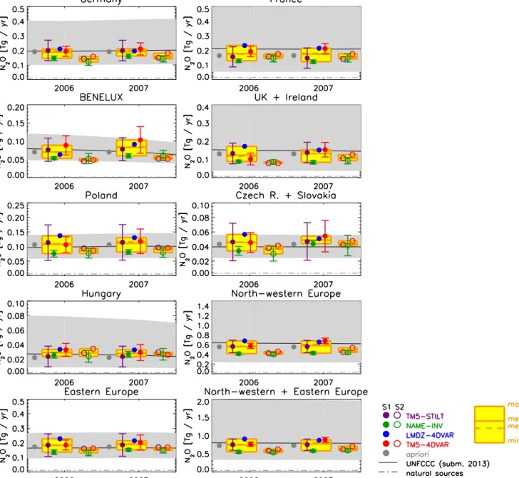
Figure 9. European N2O emissions by country and aggregated region. For each year, the left yellow box shows the results for inversion S1–
N2O, and the right yellow box for S2–N2O. The grey-shaded area is the range of UNFCCC N2O emissions (based on reported uncertainties, as compiled in Table 8; note that for some countries the UNFCCC range exceeds the scale of figures).
P. Bergamaschi et al.: Top-down estimates of European
CH
4and
N
2O emissions
25
Figure 10.
N
2O emissions over European seas. Left: total
N
2O
emissions between 35
◦and 62
◦N, and 12
◦W and 35
◦E, representing the
largest common domain of all models; right: total
N
2O emissions over the North Sea.
Figure 10. N2O emissions over European seas. Left: total N2O emissions between 35◦and 62◦N, and 12◦W and 35◦E, representing the
Table 8. N2O emissions from EDGARv4.1, EDGARv4.2 and UNFCCC for major N2O source categories. For the UNFCCC emissions, the reported relative uncertainties (2σ ) per country and category and corresponding emission ranges are also compiled. Total uncertainties per country (or aggregated countries) are estimated from the reported uncertainties per category assuming no correlation between different UNFCCC categories (but correlated errors for sub-categories). “NWE” is the total of the north-western European countries Germany, France, UK, Ireland and Benelux. “NEE” is the total of the eastern European countries Hungary, Poland, Czech Republic (CZE) and Slovakia (SVK).
Germany France UK + Ireland Benelux Hungary Poland CZE + SVK NWE NEE NWE + NEE 1A Fuel combustion
Emission (2005) EDGARv4.1 Tg N2O yr−1 0.019 0.012 0.010 0.006 0.001 0.013 0.013 0.046 0.026 0.073 Emission (2006–2007) EDGARv4.2 Tg N2O yr−1 0.018 0.011 0.010 0.005 0.001 0.012 0.006 0.044 0.020 0.063 Emission (2006–2007) UNFCCC Tg N2O yr−1 0.017 0.015 0.017 0.004 0.001 0.006 0.004 0.052 0.011 0.063 Emission range UNFCCC Tg N2O yr−1 0.012–0.021 0.009–0.021 0.001–0.046 0.001–0.011 0.000–0.001 0.005–0.008 0.001–0.008 0.023–0.098 0.006–0.017 0.029–0.115 Relative uncertainty UNFCCC 26.2 % 41.2 % 95.3–176.7 % 73.6–162.7 % 71.2 % 22.7 % 76.3 % 56.2–89.3 % 47.1 % 54.6–81.7 % 2B Chemical industry
Emission (2005) EDGARv4.1 Tg N2O yr−1 0.051 0.027 0.015 0.027 0.006 0.020 0.008 0.120 0.034 0.154 Emission (2006–2007) EDGARv4.2 Tg N2O yr−1 0.040 0.026 0.017 0.046 0.006 0.024 0.010 0.128 0.040 0.169 Emission (2006–2007) UNFCCC Tg N2O yr−1 0.031 0.019 0.008 0.025 0.004 0.015 0.008 0.083 0.026 0.109 Emission range UNFCCC Tg N2O yr−1 0.027–0.034 0.017–0.021 0.000–0.017 0.019–0.031 0.004–0.004 0.011–0.019 0.007–0.009 0.063–0.103 0.021–0.032 0.084–0.135 Relative uncertainty UNFCCC 11.1 % 10.2 % 100.0–100.4 % 24.5 % 2.2 % 29.5 % 13.9 % 23.8 % 21.1 % 23.2 % 4B Manure management
Emission (2005) EDGARv4.1 Tg N2O yr−1 0.009 0.008 0.004 0.004 0.001 0.004 0.001 0.025 0.007 0.032 Emission (2006–2007) EDGARv4.2 Tg N2O yr−1 0.009 0.008 0.004 0.004 0.001 0.004 0.001 0.025 0.006 0.031 Emission (2006–2007) UNFCCC Tg N2O yr−1 0.009 0.016 0.007 0.006 0.003 0.018 0.004 0.038 0.025 0.063 Emission range UNFCCC Tg N2O yr−1 0.004–0.016 0.008–0.024 0.000–0.033 0.000–0.011 0.000–0.006 0.000–0.045 0.002–0.006 0.012–0.083 0.002–0.057 0.014–0.140 Relative uncertainty UNFCCC 60.8-69.1 % 50.2 % 100.0–349.6 % 94.4–94.6 % 100.0–100.3 % 100.0–148.9 % 54.7–54.9 % 68.9–119.1 % 93.2–129.2 % 78.5–123.1 % 4D Agricultural soils
Emission (2005) EDGARv4.1 Tg N2O yr−1 0.086 0.098 0.077 0.025 0.012 0.052 0.013 0.285 0.077 0.363 Emission (2006–2007) EDGARv4.2 Tg N2O yr−1 0.084 0.096 0.075 0.025 0.012 0.050 0.013 0.280 0.075 0.355 Emission (2006–2007) UNFCCC Tg N2O yr−1 0.129 0.155 0.111 0.035 0.017 0.056 0.022 0.431 0.095 0.525 Emission range UNFCCC Tg N2O yr−1 0.036–0.337 0.000–0.565 0.002–0.509 0.005–0.091 0.000–0.064 0.022–0.091 0.007–0.037 0.043–1.502 0.029–0.193 0.072–1.695 Relative uncertainty UNFCCC 72.1–160.6 % 100.0–264.9 % 98.1–358.0 % 87.1–158.3 % 100.0–284.2 % 61.5 % 65.7–72.3 % 90.1–248.9 % 69.3–103.3 % 86.3–222.6 % 6B Waste water
Emission (2005) EDGARv4.1 Tg N2O yr−1 0.007 0.006 0.005 0.002 0.001 0.003 0.001 0.020 0.005 0.025 Emission (2006–2007) EDGARv4.2 Tg N2O yr−1 0.007 0.006 0.006 0.002 0.001 0.003 0.001 0.020 0.005 0.025 Emission (2006–2007) UNFCCC Tg N2O yr−1 0.008 0.003 0.004 0.002 0.001 0.004 0.001 0.017 0.005 0.023 Emission range UNFCCC Tg N2O yr−1 0.007–0.009 0.000–0.006 0.000–0.020 0.001–0.004 0.000–0.010 0.002–0.005 0.000–0.001 0.008–0.039 0.002–0.017 0.010–0.056 Relative uncertainty UNFCCC 13.8 % 100.0–104.4 % 91.1–361.1 % 70.8–75.3 % 100.0–1000.0 % 52.2 % 54.4 % 55.2–122.1 % 61.0–218.9 % 56.5–145.0 % total
total major categories EDGARv4.1 Tg N2O yr−1 0,172 0,150 0,112 0,064 0,021 0,092 0,036 0,497 0,149 0,646 Total major categories EDGARv4.2 Tg N2O yr−1 0.158 0.147 0.111 0.082 0.021 0.094 0.031 0.497 0.146 0.643 Total major categories UNFCCC Tg N2O yr−1 0.194 0.207 0.147 0.072 0.025 0.099 0.038 0.621 0.163 0.784 Total all categories UNFCCC Tg N2O yr−1 0.197 0.209 0.148 0.074 0.026 0.100 0.040 0.627 0.166 0.793 Relative uncertainty UNFCCC 48.3–107.3 % 75.0–198.2 % 75.1–271.3 % 43.9–78.1 % 67.5–192.7 % 39.8–44.6 % 38.6–42.2 % 62.9–173.0 % 43.0–63.8 % 58.5–149.8 %
is estimated to be rather small for the European countries analysed here. Given the large uncertainty of the UNFCCC inventories, the N2O emissions derived by the inverse
mod-els are surprisingly close to the UNFCCC values and the range from all models is well within the UNFCCC uncer-tainty range for all countries (or aggregated countries). The uncertainty in the UNFCCC emissions is generally domi-nated by the uncertainty in the N2O emissions from
agricul-tural soils, for which several countries estimate uncertainties well above 100 % (UK estimate: 424 %). For our estimate of the total uncertainty from the reported uncertainties per cat-egory (see Table 8), we take account of the non-symmetric nature of errors above 100 %, assuming zero emissions for the specific category as the lowermost boundary for any rel-ative error larger than 100 %. Figure 9 shows that the range of the inverse modelling estimates is much smaller than the UNFCCC uncertainty range for most countries (including the total emissions from north-western and eastern Europe). This finding is consistent with the analysis of error statistics of bottom-up inventories by Leip (2010), suggesting that the current UNFCCC uncertainty estimates of N2O bottom-up
emission inventories are likely too high.
It is important to note, however, that significant biases in N2O measurements exist between different laboratories that
require corrections (Table 7). The bias corrections calculated by TM5-4DVAR and LMDZ-4DVAR are within ∼ 0.3 ppb compared to the bias determined for those stations for which parallel NOAA discrete air measurements are available (for stations with at least 10 coinciding hourly measurements per year). This is somewhat worse than the agreement of 0.1–0.2 ppb reported by Corazza et al. (2011) and may indi-cate some limitations of the applied bias correction scheme, which does not account for potential changes of the bias within the inversion period (TM5-4DVAR: 1 year, LMDZ-4DVAR: 2 years).
Figure 11 shows the correlation coefficients and rms dif-ferences between (bias-corrected) observed and simulated N2O mixing ratios at the monitoring stations used in
inver-sion S1–N2O. The mean correlation coefficients for the four
models are in the range between 0.6 and 0.7 (averaged over all stations), which is somewhat lower than for CH4
(aver-age correlation coefficients between 0.7 and 0.8; Fig. 5). This is probably mainly due to the lower atmospheric N2O
vari-ability compared to CH4, but may be partly also due to the