HAL Id: hal-02377535
https://hal.archives-ouvertes.fr/hal-02377535
Submitted on 4 Jan 2021HAL is a multi-disciplinary open access archive for the deposit and dissemination of sci-entific research documents, whether they are pub-lished or not. The documents may come from teaching and research institutions in France or abroad, or from public or private research centers.
L’archive ouverte pluridisciplinaire HAL, est destinée au dépôt et à la diffusion de documents scientifiques de niveau recherche, publiés ou non, émanant des établissements d’enseignement et de recherche français ou étrangers, des laboratoires publics ou privés.
denudation rates
Julien Charreau, Pierre-Henri Blard, Jena Zumaque, L.C.P. Martin, Tony
Delobel, L. Szafran
To cite this version:
Julien Charreau, Pierre-Henri Blard, Jena Zumaque, L.C.P. Martin, Tony Delobel, et al.. Basinga: A cell-by-cell GIS toolbox for computing basin average scaling factors, cosmogenic production rates and denudation rates. Earth Surface Processes and Landforms, Wiley, 2019, 44 (12), pp.2349-2365. �10.1002/esp.4649�. �hal-02377535�
For Peer Review
BASINGA: a cell-by-cell GIS toolbox for computing BASIN averaGe scaling factors, cosmogenic production rates and
denudation rAtes Journal: Earth Surface Processes and Landforms Manuscript ID ESP-18-0325.R1
Wiley - Manuscript type: Research Article Date Submitted by the
Author: n/a
Complete List of Authors: CHARREAU, Julien; Université de Lorraine, CRPG Blard, Pierre-Henri; Université de Lorraine, CRPG
Zumaque, Jéna; Universite du Quebec a Montreal Geotop, Geotop Martin, Léo; University of Oslo, Department of Geosciences Delobel, Tony; Université de Lorraine, CRPG
Szafran, Lucas; Université de Lorraine, CRPG
For Peer Review
1 BASINGA: a cell-by-cell GIS toolbox for computing BASIN averaGe scaling factors, 2 cosmogenic production rates and denudation rAtes
3
4 Julien Charreau1**, Pierre-Henri Blard1, Jéna Zumaque1,2, Léo C.P. Martin1,3, Tony Delobel1 and Lucas Szafran1 5
6 1. CRPG, UMR 7358, CNRS, Université de Lorraine, 54501 Vandoeuvre-lès-Nancy, France,
charreau@univ-7 lorraine.frr, [email protected], [email protected], [email protected]
8 2. Geotop, Université de Québec à Montréal, CP 8888, Succ. Centre Ville Montréal, Québec, Canada,
10 3. Department of Geosciences, University of Oslo, P.O. Box 1047, Blindern, 0316 Oslo, Norway,
12
13 **corresponding author: Julien Charreau ([email protected])
14
15 Abstract
16 The calculation of denudation rates from the measured cosmogenic nuclide concentrations
17 in river sediments requires assumptions and approximations. Several different approaches and
18 numerical tools are available in the literature. A widely used analytical approach represents the
19 muogenic production with one or two exponentials, assumes the attenuation length of muons to
20 be constant and also neglects temporal variations in the Earth magnetic field. The denudation
21 rates are then directly and analytically calculated from the measured concentrations. A second
22 numerical and iterative approach was more recently proposed and considers a more rigorous
23 muogenic production laws based on pre-calculated variable attenuation length of muons and
24 accounts for temporal changes of the magnetic field. It also assumes a specific distribution of
25 denudation rates throughout the basin and uses an iterative approach to calculate the basin
26 average denudation rates.
27 We tested the two approaches across several natural basins and we found that both
28 approaches provide similar denudation results. Hence, assuming exponential muogenic
29 production and constant attenuation length of muons in the rock has little impact on the derived
30 denudation rates. Therefore, unless a priori known distributions of denudation rates are to be
31 tested, there does not appear to be any particular gain from using the second iterative method
32 which is computationally less effective.
3 4 5 6 7 8 9 10 11 12 13 14 15 16 17 18 19 20 21 22 23 24 25 26 27 28 29 30 31 32 33 34 35 36 37 38 39 40 41 42 43 44 45 46 47 48 49 50 51 52 53 54 55
For Peer Review
33 Based on these findings, we developed and describe here Basinga, a new ArcGIS® and
34 QGIS toolbox which computes the basin average scaling factors, cosmogenic production rates
35 and denudation rates for several tens of drainage basins together. Basinga follows either the
36 Lal/Stone or the LSD scaling schemes and includes several optional tools for correcting for
37 topographic shielding, ice cover and lithology. We have also developed an original method for
38 correcting the cosmogenic production rates for past variations in the Earth's magnetic field.
39
40 key words: scaling factors, cosmogenic production rates, denudation rates, ArcGIS and QGIS
41
42 1. Introduction
43 Denudation is a critical parameter controlling the landscape evolution. It can be
44 determined at the scale of an entire watershed from the cosmogenic nuclides concentration
45 measured in one river sediment sample (e.g. Brown et al., 1995). This method has consequently
46 been widely used in a variety of geological settings (Portenga and Bierman, 2011). The
47 calculation of denudation rates from measured concentrations in sediments relies on specific
48 assumptions and requires computation of several parameters, notably the cosmogenic production
49 rates at the surface of the drainage basin. The physical characteristics of these production rates
50 can be estimated from a number of analytical, empirical or physical formulations. Consequently,
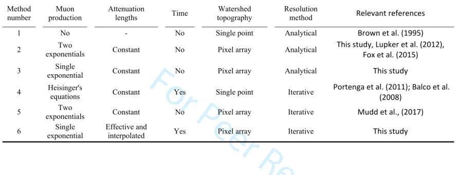
51 in the literature, the approaches adopted vary between authors and studies, leading to potential
52 discrepancies (Table 1) (e.g. Brown et al., 1995; Fox et al., 2015; Godard et al., 2012; Lupker et
53 al., 2012; Mudd et al., 2016; Portenga and Bierman, 2011; Scherler et al., 2014). In this paper,
54 we first review the different approaches, the associated assumptions and the formulae used to
55 calculate the basin average denudation rates, and we test their sensitivity. From these results, we
56 define a strategy to estimate the true basin average denudation rates and find the best balance
57 between the computational time of the methods and their accuracy. Accordingly, we have
58 developed and present here a free, simple and open-source tool that provides an accurate and
59 efficient means for computing the basin average denudation rates under different assumptions
60 and scaling models. It is named Basinga (BASIN-averaGe scaling factors, cosmogenic
61 production and denudation rAtes) and includes two Python-script-based geoprocessing tools that
62 can calculate both the cosmogenic production rates and the denudation rates. These tools use two
3 4 5 6 7 8 9 10 11 12 13 14 15 16 17 18 19 20 21 22 23 24 25 26 27 28 29 30 31 32 33 34 35 36 37 38 39 40 41 42 43 44 45 46 47 48 49 50 51 52 53 54 55
For Peer Review
63 simple and user-friendly graphical interfaces that can be installed and run on two widely used
64 GIS systems: ArcGIS® and QGIS.
65
66 2. Denudation rates from the cosmogenic concentration
67 2.1 General formulation
68 At any location, the concentration N (atoms.g-1) of a cosmogenic nuclide i in a surface 69 rock (z=0) can be related to the exposure duration t (a) (present is 0 and positive toward the past)
70 and the local denudation rate ε (cm.a-1) following this general equation (e.g. Balco, 2017):
71 𝑁𝑧 = 0, 𝑖= ∑𝑥 = 𝑠𝑝,𝜇∫ (1)
∞
0𝑃𝑥, 𝑖(𝜀𝑡)𝑒 ― 𝜆𝑖𝑡𝑑𝑡
72 where the subscript i and x indicate the studied cosmogenic nuclide (e.g. 10Be, 26Al, 3He, 21Ne) 73 and the cosmogenic production pathway (sp for production by spallation; for slow muon 𝜇
74 capture and fast muon processes), respectively. is the decay constant of the studied nuclide 𝜆𝑖 75 (4.9975 10-7a-1 for 10Be;(Chmeleff et al., 2010)). P
x,i, is the local in situ cosmogenic production 76 rates at the surface (at.g-1.a-1) of the production mechanism associated with each pathway x. The 77 depth production due to spallation follows an exponential (Lal, 1991), then the equation (1) can
78 be rewritten as follow: 79 𝑁𝑧 = 0, 𝑖= (2) 𝑃𝑠𝑝,𝑖 𝜌𝜀 Λ𝑠𝑝,𝑖 + 𝜆𝑖 𝑒―( 𝜌𝜀 Λ𝑠𝑝,𝑖 + 𝜆𝑖)𝑡+ ∫∞ 0𝑃𝜇, 𝑖(𝜀𝑡)𝑒 ― 𝜆𝑖𝑡𝑑𝑡
80 where ρ and Λsp,i are the rock density (g.cm-3) and the attenuation length of fast neutron 81 production (g.cm-2), respectively. This later theoretically varies with latitude and elevation, and 82 more specifically with atmospheric depth and cut-off rigidity (Gosse and Phillips, 2001; Lal,
83 1991; Marrero et al., 2015; Sato et al., 2008; Stone, 2000). It is however difficult to constrain
84 with accuracy, and therefore it is often convenient to assume a constant value of 160 g.cm-2 for 85 Λsp,i (e.g. Braucher et al., 2011).
86 The first term of this equation (2) that represents the spallogenic production is generally
87 simplified in 𝜌𝜀𝑃𝑠𝑝,𝑖 , assuming that there is no inherited cosmogenic nuclide before exposure
Λ𝑠𝑝,𝑖 + 𝜆𝑖
88 initiation and that the cosmogenic nuclide concentration has reached steady state (i.e. t>>1/(λ +
89 ερ/Λ) (Brown et al., 1995; Lal, 1991). In some conditions, the denudation may not be at steady
90 state and hence the denudation rates derived from this assumption can be biased (e.g. Bierman
91 and Steig, 1996). However, the potential inaccuracy due to the violation of this assumption is
3 4 5 6 7 8 9 10 11 12 13 14 15 16 17 18 19 20 21 22 23 24 25 26 27 28 29 30 31 32 33 34 35 36 37 38 39 40 41 42 43 44 45 46 47 48 49 50 51 52 53 54 55
For Peer Review
92 significant (30 to 50%) only in very slowly eroding landscapes (<10-3 cm/a) but remain below 93 few percent in most of the other geological contexts (Bierman and Steig, 1996; Schaller and
94 Ehlers, 2006).
95 The second term of equation (2) represents the muogenic contribution, which includes two
96 different production pathways (slow muon capture and fast muon processes). Rigorously, the
97 depth-dependence production rates of these particles do not follow a simple exponential
98 attenuation (Heisinger et al., 2002a, 2002b). Equation (2) should include a rigorous calculation of
99 the muogenic contribution following the Heisinger's equations (Heisinger et al., 2002a, 2002b)
100 (see for example equations 5 and 6 in Balco, 2017).
101 Assuming that a river mixes the sediments eroded across the whole drainage basin well,
102 the concentration measured at the river outlet represents the basin average of all local
103 concentrations (Brown et al., 1995; Lal, 1991). By solving and integrating equation (2) over the
104 basin surface, it is therefore possible to derive the average denudation rate at the basin scale from
105 a measured cosmogenic nuclide concentration in a river sediment (Brown et al., 1995; Lal, 1991),
106 provided that the cosmogenic production rates of the nuclide at the surface (Px,i) are known at 107 each point of the basin.
108
109 2.2 The cosmogenic production rates and scaling factors
110 The in situ spallogenic production of cosmogenic nuclides at the surface is a function of
111 the longitude, but more importantly of the latitude L (°), since it is primarily controlled by the
112 quantity of cosmic flux that reaches the high atmosphere and is therefore driven by the strength
113 of the geomagnetic field and the cut-off rigidity of the incoming particles (Lal, 1991). Moreover,
114 temporal variations in the Earth's magnetic field (e.g. Valet et al., 2005) are responsible for
115 changes in the cosmic flux (Dunai, 2001; Nishiizumi et al., 1989; Pigati and Lifton, 2004) and
116 hence in the spallogenic production rates. The cosmogenic nuclide concentration measured at the
117 surface is integrated over an equivalent exposure time, which represents the time needed by the
118 grain to reach the surface while it is subjected to cosmic ray bombardment. This duration depends
119 on the denudation rate and the attenuation length: teq=1/(+/). However, the Earth’s 120 magnetic field has negligible impact on muon fluxes and hence on muogenic production (e.g.
121 Balco et al., 2008; Braucher et al., 2011; Lifton et al., 2014). Both production pathways are a
122 function of the elevation since the secondary fluxes produced in the high atmosphere are
3 4 5 6 7 8 9 10 11 12 13 14 15 16 17 18 19 20 21 22 23 24 25 26 27 28 29 30 31 32 33 34 35 36 37 38 39 40 41 42 43 44 45 46 47 48 49 50 51 52 53 54 55
For Peer Review
123 attenuated both in flux and energy by the atmosphere (Lal, 1991). In the calculations, elevation is
124 usually converted to the equivalent atmospheric depth h (g.cm-2) (Stone, 2000), which can be 125 calculated either using the hydrostatic standard atmosphere model specific to mid-latitude and the
126 northern hemisphere (see Equation (1) in Stone (2000)) or can been interpolated from the
127 atmospheric 2D ERA-40 database (Uppala et al., 2005).
128 The rate of cosmogenic production at the surface (at.g-1.a-1) at any location within a given 129 watershed can be scaled to the latitude, elevation and time as follows:
130 𝑃𝑖,𝑥= 𝑃𝑖,𝑥,𝑆𝐿𝐻𝐿 . 𝑆𝑖,𝑥(ℎ,𝐿,𝑡(𝜀)) (3)
131 where 𝑃 is the surface production at Sea Level and High Latitude (SLHL) (at.g-1.a-1) for 𝑖,𝑥,𝑆𝐿𝐻𝐿
132 each nuclide i and production pathway x. Global average values for the SLHL production rates of
133 different nuclides have recently been constrained by Martin et al. (2017) (see table 7), taking into
134 account all published calibration studies, notably the most recent ones (Balco et al., 2009;
135 Kaplan et al., 2011; Kelly et al., 2015; Lifton et al., 2014; Martin et al., 2015; Stroeven et al.,
136 2015). These worldwide averages were computed using the CREp program (Martin et al., 2017)
137 and include a time-integration correction based on the VDM reconstructed by Muscheler et al.
138 (2005).
139 In equation (3), Si,x represents the scaling factor for each production pathway x and each 140 studied nuclide i. Several empirical scaling models have been proposed in the literature. Some of
141 them were calibrated from the counting of spallation events by either photo-emulsion (e.g. Lal,
142 1991; Stone, 2000) or neutron-monitor (Desilets et al., 2006; Dunai, 2001; Lifton et al., 2005).
143 However, more recently, a purely theoretical and physical ab initio model was developed by
144 Lifton/Sato/Dunai (LSD) to describe the temporal and spatial variability in cosmogenic
145 production (Lifton et al., 2014).
146 For computational efficiency, previous studies (e.g. Fox et al., 2015; Godard et al., 2014;
147 Scherler et al., 2014; Wittmann and von Blanckenburg, 2009) have often calculated the
148 production rates using the widely used and accessible empirical scaling scheme of Lal/Stone (Lal,
149 1991; Stone, 2000). Considering the worldwide calibration dataset, statistical analyses show that
150 the Lal/Stone model has a better accuracy than the neutron-monitor-based schemes (Balco, 2017;
151 Borchers et al., 2015; Phillips et al., 2016). These analyses also show that, despite regional
152 differences, the Lal/Stone model has a similar efficiency than the LSD model (Borchers et al.,
153 2015; Lifton et al., 2014). 3 4 5 6 7 8 9 10 11 12 13 14 15 16 17 18 19 20 21 22 23 24 25 26 27 28 29 30 31 32 33 34 35 36 37 38 39 40 41 42 43 44 45 46 47 48 49 50 51 52 53 54 55
For Peer Review
154 However, calibration sites remain too sparse to accurately unravel the full differences
155 between these two models at the global scale (Figs. 1 and 2). To estimate the spatial variability
156 and the agreement between the two models, we calculated the difference between the two scaling
157 models for the entire world, using as inputs the 2D ERA atmosphere database (Uppala et al.,
158 2005) and the Global Multi-resolution Terrain Elevation Data 2010 (GMTED2010) (Danielson
159 and Gesch, 2011). In most regions the two models differ by less than 10% on average, especially
160 at mid-latitude and moderate elevation (1-4 km) (Figs. 1 and 2). At high altitude/high latitude and
161 low altitude/low latitude the discrepancy between the two models may reach ~20-30% (Figs. 1
162 and 2) (Phillips et al., 2016). The difference also varies strongly with altitude (Fig. 1).
163
164 3. Approaches and assumptions for computing basin average denudation rates
165 The equations (1) and (2), that link the denudation rate to the cosmogenic concentration at
166 the surface, are rigorously implicit in . To calculate the basin average denudation rate from the
167 cosmogenic concentration measured at the outlet, assumptions and approximations must therefore
168 be made and two sorts of approach (analytical or numerical) have been developed for this (Table
169 1) (Balco et al., 2008; Brown et al., 1995; Mudd et al., 2016).
170
171 3.1 Analytical approaches
172 The first type of approach, which are traditionally used in the literature, either neglects the
173 muogenic production (method 1 in Table 1) or approximates, similarly to the spallogenic
174 production, the two muogenic production rates at depth with either one or two different
175 exponential laws (methods 2 and 3 in Table 1) (e.g. Braucher et al., 2011; Lupker et al., 2012).
176 Then, the equation (2) can be simplified as follow:
177 𝑁𝑧 = 0, 𝑖= ∑𝑥 = 𝑠𝑝, 𝜇𝑠𝑚, 𝜇𝑓𝑚 (4)
𝑃𝑥,𝑖 𝜌𝜀 Λ𝑥,𝑖 + 𝜆𝑖
178 where 𝜇𝑠𝑚 and 𝜇𝑓𝑚 indicate the two muogenic production pathways. This approach may use the
179 constant attenuation lengths of 4320 g/cm2 and 1500 g/cm2 determined by Braucher et al. (2011) 180 using the experimental data of Heisinger et al. (2002a,b) for fast muons capture and slow muons
181 processes, respectively (method 2). If only one family of muons is considered with a single
182 exponential then one single constant attenuation length in the rocks can be used (method 3) (see
183 table 2 in Braucher et al., 2013).
3 4 5 6 7 8 9 10 11 12 13 14 15 16 17 18 19 20 21 22 23 24 25 26 27 28 29 30 31 32 33 34 35 36 37 38 39 40 41 42 43 44 45 46 47 48 49 50 51 52 53 54 55
For Peer Review
184 This first type of approach (methods 1,2 and 3) also assumes no temporal variation in the
185 Earth’s magnetic field. In such a case, equation (4) can be directly solved analytically (Brown et
186 al., 1995). The basin average denudation rate is only a function of the concentration measured at
187 the outlet and the present average cosmogenic production rate of the basin (e.g. Brown et al.,
188 1995). In the literature, the latter is sometimes estimated from the mean altitude and latitude of
189 the studied catchment area (method 1) (Brown et al., 1995). However, because the production
190 rate vs. elevation relationship is non-linear, such an approximation may induce significant
191 uncertainties (>30%), especially in high elevation regions with high relief in the drainage basins.
192 To avoid these inaccuracies, it is critical to consider the whole basin topography (Balco et al.,
193 2008). A more accurate method scales the factors and hence the production rates on a pixel basis
194 using a Digital Elevation Model (DEM) and a cell-by-cell approach (methods 2 and 3) (e.g. Fox
195 et al., 2015; Godard et al., 2012; Lupker et al., 2012). The average production at the basin scale
196 can then be easily calculated to derive the basin average denudation rate.
197
198 3. 2 Iterative numerical approaches
199 The second type of approach solves the equation (2) numerically in order to provide the
200 denudation rates (e.g. Balco et al., 2008) (methods 4,5 and 6 in Table 1). Indeed, based on this
201 equation and using the Heisinger's formulation of the muogenic production (Heisinger et al.,
202 2002a, 2002b), it is possible to compute a theoretical cosmogenic concentration only if the
203 denudation is a priori known. Then, the denudation rate can be adjusted iteratively in order to
204 minimize the discrepancy between the measured and calculated concentrations (method 4). This
205 iterative methodology is available in the updated online calculator of Balco et al. (2008)
206 (http://hess.ess.washington.edu/). One advantage of this method is that the exposure duration can
207 be calculated from the input denudation at each iteration and, thus, the cosmogenic production
208 rate can be corrected for temporal variations in the Earth’s magnetic field (Balco et al., 2008).
209 However, the initial code of Balco et al. (2008) was designed for the calculation of local
210 denudation rates only (method 4).
211 To extrapolate this iterative technique at the basin scale one must assume that the
212 denudation is homogenous (Mudd et al., 2016; Scherler et al., 2014) or specify a known
213 distribution of denudation throughout the basin. Otherwise, there would be an infinite number of
214 denudation distribution solutions throughout the basin that could be possible. Based on this a
3 4 5 6 7 8 9 10 11 12 13 14 15 16 17 18 19 20 21 22 23 24 25 26 27 28 29 30 31 32 33 34 35 36 37 38 39 40 41 42 43 44 45 46 47 48 49 50 51 52 53 54 55
For Peer Review
215 priori known denudation distribution (homogenous or specified) the production rates can be 216 corrected for temporal variations in the Earth’s magnetic field. Again, as for the previous
217 approaches (methods 1,2 and 3), this method requires calculation of the cosmogenic production
218 rates for both production pathways (spallogenic and muogenic) at each location in the basin, and
219 this must also be made on a pixel basis using a DEM. The concentration of a cosmogenic nuclide
220 at each location and the basin average concentration could then be calculated accordingly. The
221 denudation rate of the basin could then be adjusted iteratively in order to minimize the
222 discrepancy between the measured and calculated concentrations at the outlet. To use this
223 iterative methodology at the basin scale one would need to calculate the muogenic production
224 using Heisinger's equations at each point of the basin, which is a time-consuming computation.
225 Therefore, such an approach still needs to be fully developed for the calculation of basin average
226 denudation rates. Indeed, though Mudd et al. (2016) have developed an iterative methodology,
227 they assumed a constant attenuation length for muons and considered only present-day
228 production rates derived from the Lal/Stone model, without any correction for temporal
229 variations (method 5 in Table 1).
230 Alternatively, the right muogenic production can be calculated using Heisinger's
231 formulations (Heisinger et al., 2002a, 2002b) for a reasonable range of denudation rates and
232 atmospheric depth values and, hence, the attenuation length of muons can be derived accordingly
233 assuming a single exponential law (see equation 12 of Balco, 2017) (Fig. 3). Based on these
pre-234 calculated values, the attenuation length of muons can be interpolated at each point of a given
235 drainage basin using elevations and denudations grids. The cosmogenic concentration can be then
236 more quickly but relatively accurately estimated at each point of the studied basin. The denudation
237 rate can be then derived using the same iterative technic than in method 4 and 5 (method 6).
238
239 4. Sensitivity analysis
240 It is worth testing and comparing the accuracies of the two types of approach. Moreover,
241 it is still unclear if the new LSD model would yield any significant differences when calculating
242 basin average denudation rates.
243 244 4.1 Approach 3 4 5 6 7 8 9 10 11 12 13 14 15 16 17 18 19 20 21 22 23 24 25 26 27 28 29 30 31 32 33 34 35 36 37 38 39 40 41 42 43 44 45 46 47 48 49 50 51 52 53 54 55
For Peer Review
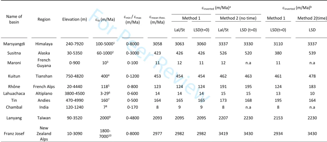
245 To discriminate between the two types of approach and the two scaling models, we
246 considered several natural catchments across the world, notably in regions where the two scaling
247 schemes differ strongly (Table 2), in particular at high latitude/high elevation (i.e. the Susitna
248 basin in Alaska) and at low latitude/low elevation (the Maroni basin in the French Guyana,
0-249 900m at ~4°N) (Fig. 1). We also tested several basins that exhibit a wide elevation range (i.e.
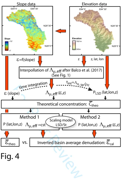
250 Marshyangdi, Kuitun). At each cell in a basin, we assumed that denudation was a linear function
251 of the local slope. We then arbitrarily set the maximum denudation rate so that the basin average
252 denudation rate roughly equaled the rates reported in the literature, which were derived from
253 thermochronology, sediment gauging and/or TCN analysis (see the complete list of references
254 given in Table 2) (Fig. 4).
255 Based on these a priori known denudation rate distributions, we applied a forward model
256 to calculate the theoretical "true" in situ 10Be concentrations at each cell in the basins. We used 257 both the LSD (Lifton, 2015) and Lal/Stone (Lal, 1991; Stone, 2000) schemes to estimate the
258 scaling factors and production rates in each cell based on the cell’s latitude, longitude and
259 elevation. For the LSD model, we used the Matlab® functions of Lifton et al. (2015), which were 260 amended by Martin et al. (2017) to test for different dipolar geomagnetic corrections. When using
261 the Lal/Stone scheme the time was not integrated and we used only the present-day scaling
262 factors. For LSD, we considered both the present-day factors and factors corrected for variations
263 in the Earth’s magnetic field. In such a case, the time was integrated for each cell based on the
264 equivalent time derived from the denudation itself. Atmospheric depth was always calculated
265 using the data from the 2D ERA-40 database (Uppala et al., 2005). 10Be cosmogenic production 266 rates were calculated based on the SLHL rate of 4.11 of Martin et al. (2017) (see their Table 7).
267 We followed the approach and database proposed by Balco (2017) to accurately estimate the
268 attenuation length of muons in the rocks as a function of the denudation and elevation (Fig. 4).
269 Next, we calculated the basin average "true" concentration using equation (4). These values were
270 then inverted using the two types of approach (method 3 vs. 5) to estimate the basin average
271 denudation rates for each basin accordingly. For consistency, the inversions considered the same
272 scaling as that used during the calculation of the theoretical concentration. For the iterative
273 approach, the distribution of the denudation was assumed to be homogenous throughout the
274 basin. Since the attenuation length of muons as a function of denudation and elevation can only
275 be calculated for all muons together, in the analytical approach we therefore considered only one
3 4 5 6 7 8 9 10 11 12 13 14 15 16 17 18 19 20 21 22 23 24 25 26 27 28 29 30 31 32 33 34 35 36 37 38 39 40 41 42 43 44 45 46 47 48 49 50 51 52 53 54 55
For Peer Review
276 single family of muons and used the method 3 with constant attenuation length in the rocks. We
277 used the value of 4814 g.cm-2 which represents the mean of the attenuation lengths given in 278 Braucher et al. (2013). Finally, we compared the inverted average denudation results to the input
279 theoretical values.
280
281 4.2 Results
282 The complete results are given in table 2 and figures 5, 6 and 7 show the results for
283 representative basins. For most of the studied basins, we found that the analytical approach
284 (method 3) (which assumes the attenuation length of muons to be constant) provided denudation
285 rate estimates that were on average better than or similar to those of the iterative approach,
286 whatever the scaling model used. Adding the temporal modulation of the production rates led to
287 larger misfits between the denudation rates calculated using the analytical approach (which uses
288 the present rates) and the theoretical denudation rates. However, the iterative approach, which
289 can account for these modulations, did not provide better results (Table 2) and for several basins
290 it yielded large differences (10-20%)(Fig. 5). When we used the scaling models for inversion
291 without time integration ahead, meaning that only the attenuation length of muons differed
292 between the theoretical calculation and the inversion, the differences between the theoretical and
293 inverted denudation rates were on average negligible except for basins with very low denudation
294 rates (i.e. Maroni and Chambal), where the differences were significant (<10%).
295
296 5. Discussion and implementation in Basinga
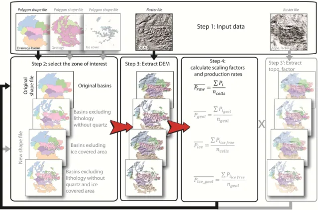
297 5.1 Goals of Basinga
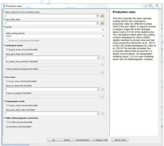
298 The first aim of Basinga (BASIN-averaGe scaling factors, cosmogenic production and
299 denudation rAtes) was to provide a tool, named "Production rate", for computing cosmogenic
300 production rates for different nuclides (3He, 21Ne and 10Be). The second goal of Basinga was to 301 calculate, for a large number of drainage basins together, the mean denudation rates from the
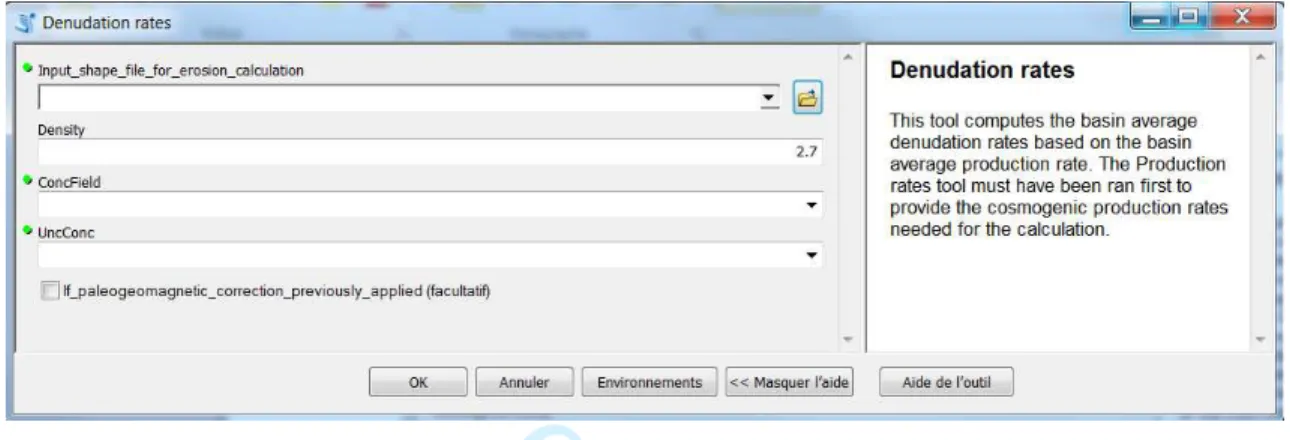
302 cosmogenic concentrations measured at their outlet. Hence, a second tool named "Denudation
303 rates" was designed. Our main objective was to provide, for both tools, simple and user-friendly 304 graphical interfaces that could be installed on GIS systems and run using simple Digital Elevation
305 Model (DEM) raster and shape files of the drainage basins. Based on the above methodological
306 analysis, we therefore developed Python-script-based geoprocessing tools that can be run and
3 4 5 6 7 8 9 10 11 12 13 14 15 16 17 18 19 20 21 22 23 24 25 26 27 28 29 30 31 32 33 34 35 36 37 38 39 40 41 42 43 44 45 46 47 48 49 50 51 52 53 54 55
For Peer Review
307 installed on two widely used and/or free GIS systems, ArcGIS® and QGIS. These tools calculate
308 the cosmogenic production and denudation rates for several nuclides, based on two possible
309 scaling models and using several corrective options that were built to improve the accuracy of the
310 estimates. However, all of these methodological improvements and associated potential gain in
311 accuracy must be handled with caution, given the uncertainties associated to the cosmogenic
312 method itself, especially in low eroding landscape (<0.001 cm/a) (Bierman and Steig, 1996). A
313 detailed description of Basinga, its interfaces and how they can be used are given in the
314 Supplementary information.
315
316 5.2 Choice of the scaling model
317 At moderate altitudes (1000-6000m), the differences between the two scaling models are
318 in general quite low (<10%). Hence, for basins of high relief at moderate elevation (e.g.
319 Marshyangdi, Susitna, Kuitun), the weights of the extreme scaling values are likely negligible
320 and the higher production rates at lower elevations derived using Lal/Stone are compensated for
321 by the lower production rates at high elevation (Figs. 6 and 7). Moreover, the true difference
322 between the two scaling models is likely lower than our modeling suggests because at high
323 elevation, where the discrepancies between the models are greater, cosmogenic production is
324 partially canceled out by ice cover that shields surficial rocks from cosmic rays. The other
325 sources of random uncertainty associated with the cosmogenic measurements are equivalent to
326 the bias computed in our simulation (ca. 5 to 10%). Therefore, given the other geological
327 uncertainties such as those related to the steady state assumption (Bierman and Steig, 1996;
328 Schaller and Ehlers, 2006), for most natural cases, the choice of the scaling model will have little
329 impact. Since it is computationally more efficient to follow the Lal/Stone model for calculating
330 the cosmogenic production rates, we would encourage use of this model in most of the cases.
331 Nevertheless, precautions must be taken when studying drainage basins or sub-catchments
332 of low relief in regions where the difference between the two scaling models is rather high
(15-333 30%). For example, in the Maroni and Chambal basins, because of the low relief (0-1000m) and
334 low latitude, the difference between the scaling models is significant everywhere and the extreme
335 values are not compensated by each other. The resulting difference in denudation rates remains
336 significant (~15%). Unfortunately, the calibration data remain too sparse in these particular
337 regions to determine which of the two models is more accurate (Phillips et al., 2016; Martin et al.,
3 4 5 6 7 8 9 10 11 12 13 14 15 16 17 18 19 20 21 22 23 24 25 26 27 28 29 30 31 32 33 34 35 36 37 38 39 40 41 42 43 44 45 46 47 48 49 50 51 52 53 54 55
For Peer Review
338 2017). In such cases, and until new discriminant calibration data are provided, both scaling
339 models should be used to provide a realistic range of possible denudation values. However, if the
340 expected denudation rates of the studied low relief region are low (<0.001 cm/a), the difference
341 between the two estimates will likely be in the range of the uncertainties associated to the
342 precision of the cosmogenic method itself (Bierman and Steig, 1996).
343 The Basinga tool Production rates thus allows the user to calculate the scaling factors and
344 the production rates using either the LSD or the Lal/stone model. The LSD model was
345 implemented in Python using the Matlab functions of Lifton et al. (2014) modified by Martin et
346 al. (2017). The Production rates tool calculates the basin average production rates based on the
347 SLHL rates provided in Martin et al. (2017) (see their table 7) as a function of the studied nuclide
348 and the scaling model and derived from the ERA40 atmosphere database. For 21Ne the SLHL is 349 calculated from the 10Be SLHL rate and a 10Be/21Ne ratio of 4.12 (Kober et al., 2011). The SLHL 350 for each particles are calculated based on their relative production rate to the total production at
351 sea level high latitude with values of 98.86%, 0.27% and 0.87% for spallation, slow muon
352 capture and fast muon processes, respectively (see table Table 1 of Martin et al., 2017 and
353 Braucher et al., 2011).
354 Nevertheless, the SLHL values can be easily updated and modified in the program file if
355 needed using a simple text editor (see Online supplementary information and the section "Getting
356 Started" for the procedure and which lines to change). For example, local or regional SLHL
357 values can be used, as derived from the CREp program and using a compilation of local
358 calibration sites (Martin et al., 2017).
359 However, calculation of the production rates using LSD may take several hours for an
360 average sized drainage basin of few thousand km2 (Fig. 8). For large catchments, for example the 361 Gangese (9.0105 km2), the Amazon (6.9106 km2) or the Rhône (9.7104 km2), the computing 362 time can be very long (Fig. 8) and the computation may be difficult to perform on a simple laptop
363 computer. The same is true if a large number of basins are analyzed together. In such cases, the
364 resolution of the analyzed DEM needs to be increased, which could generate a potential source of
365 inaccuracy. Use of the LSD model is therefore for now limited to basins of small size.
366
367 5.3 An alternative approach for estimating the LSD scaling factors
3 4 5 6 7 8 9 10 11 12 13 14 15 16 17 18 19 20 21 22 23 24 25 26 27 28 29 30 31 32 33 34 35 36 37 38 39 40 41 42 43 44 45 46 47 48 49 50 51 52 53 54 55
For Peer Review
368 To overcome this issue and to reduce the computing time when using the LSD model, we
369 can lean on the simple relationship that exists, at the basin scale, between the Lal/Stone and the
370 LSD scaling factors (Figs. 2, 6 and 7). If time is not integrated to correct for past changes in the
371 Earth’s magnetic field, the relationship between the two models can be approximated by a simple
372 polynomial law for each basin (Figs. 6 and 7). The spallogenic and muogenic factors for both
373 models can be calculated together over a small number of cells that are randomly sampled within
374 the studied basin. These data can then be used to find the best fit relationship between the two
375 models for each production pathway. The LSD factors on the other cells are then calculated using
376 these conversion laws and the previous Lal/Stone factors that had been quickly estimated for each
377 cell. Our tests show that a 4 degree polynomial fit derived from 1000 sampled cells provides an
378 accurate law for estimating the LSD factors of the whole basin (the average bias is lower than
379 1%, and never exceeds 3%) (Fig. 9). This alternative approach significantly reduces the
380 computing time needed to calculate the LSD scaling factors when time is not integrated (Fig. 8).
381 A similar approximation of the LSD factors based on a pre-calculated table is also used in the
382 updated online calculator of Balco et al. (2008) (http://hess.ess.washington.edu/). When using the
383 LSD model in Basinga, this simplification can be activated if desired.
384
385 5.4 Chosen methodology for denudation inversion
386 Though we analyzed ten natural basins in different settings, because the controlling
387 factors are multiple (denudation, hypsometry, reliefs, latitude, longitude etc) our results cannot
388 easily be generalized. Since the calculations are relatively long for each basin, especially when
389 using the iterative approach, it is difficult to multiply the studied cases to encompass all possible
390 variations in all of these factors. To discriminate between the two methods, the net influence of
391 the attenuation length of muons in the rocks is critical. However, the sensitivity of the denudation
392 rate to this parameter can be tested more systematically using the Lal/Stone model, which is
393 computationally more efficient. In such a case, it is computationally possible to vary the
394 maximum altitude (hence its relief), the mean latitude and the denudation distribution of a given
395 basin of relatively small size. We considered here a smaller sub-basin of the Marshyangdi and
396 fixed its hypsometry while the other parameters were varied. We tested about 300 different cases
397 with mean latitudes, reliefs and denudation rates ranging from 5 ° to 55°, 450 to 4500m and 0.01
398 to 0.4 cm/a, respectively. The differences between the inverted and theoretical denudation are on
3 4 5 6 7 8 9 10 11 12 13 14 15 16 17 18 19 20 21 22 23 24 25 26 27 28 29 30 31 32 33 34 35 36 37 38 39 40 41 42 43 44 45 46 47 48 49 50 51 52 53 54 55
For Peer Review
399 average less than 1% (Fig. 10). These results also suggest that assuming a constant attenuation
400 length of 4814 g.cm-2 (Braucher et al., 2013) has negligible impact on the final denudation results 401 in a wide range of settings. However, for very low denudation rates (<0.01 cm/a) at low altitude
402 (<1000m), as for example in the Maroni and Chambal basins, the effective attenuation length
403 derived by Balco (2017) is significantly lower than Braucher's value (Fig. 1), resulting in larger
404 discrepancies between theoretical and inverted denudation rates. The discrepancy still remains
405 lower than <10% however (Fig. 10). These results reinforce the conclusion that the analytical
406 approach provides relatively accurate results even if variations in the attenuation length of muons
407 are neglected.
408 Moreover, the analytical approach has the advantage of being straightforward and
409 computationally faster even when using the LSD model. In contrast, the numerical and iterative
410 approach requires, at each step, the attenuation length of muons from the tested denudation to be
411 re-computed for each cell. If the temporal fluctuations in the production rates are integrated, the
412 associated computation must also be performed at each step as function of the tested denudation
413 rates. The time needed to compute the scaling factors is hence significantly increased and the
414 calculation may take several tens of hours for a basin of average size when using the
time-415 dependent version of the LSD model (Fig. 8).
416 At last, the potential gain in accuracy that could results from considering variations in the
417 attenuation length of muons is likely negligible compared to the natural geological uncertainties.
418 Nevertheless, the iterative approach merits consideration if an a priori known distribution
419 of denudation is available, derived for example from shear stress, lithology data or output from
420 numerical landscape models. In such a case, the tool developed by Mudd et al. (2016), which is
421 freely available online, may be used. However, this tool is based on the Lal/stone model only and
422 also assumes a constant attenuation length of muons. A complete iterative tool, with a variable
423 attenuation length of muons and based on the LSD model including time integration, has yet to be
424 developed.
425 If the distribution of denudation is a priori unknown, the use of the analytical approach is,
426 in our opinion, sufficient and more efficient. Unfortunately, no simple and freely available tool
427 has been provided for this approach. Consequently, our second Python script, Denudation rates,
428 follows the analytical approach and uses the method 2 (Table 1) with the muogenic production
429 represented by two exponentials. To calculate the denudation rates for each basin studied,
3 4 5 6 7 8 9 10 11 12 13 14 15 16 17 18 19 20 21 22 23 24 25 26 27 28 29 30 31 32 33 34 35 36 37 38 39 40 41 42 43 44 45 46 47 48 49 50 51 52 53 54 55
For Peer Review
430 Denudation rates requires the measured concentration of the in situ cosmogenic nuclide at the 431 outlet and the calculation of the basin average production rates before. These basin averages are
432 provided by the Production rates tool using a DEM projected in a geographical system with the
433 area of each individual cells of the DEM corrected for latitudinal effects.
434
435 5.5 An approach for integrating time and changes in the Earth’s magnetic field using the
436 analytical approach
437 Theoretically, the analytical approach precludes any accounting for past changes in the
438 Earth’s magnetic field because the production rates are calculated for the present time only. In
439 many mountain ranges, such as in Taiwan, the Himalayas or the New Zealand Alps, denudation
440 rates are usually high and exceed 0.1-0.2 cm/a (Derrieux et al., 2014; Herman et al., 2010;
441 Lupker et al., 2012). In such cases, the equivalent exposure times are low (<400 a) and the
442 associated biases likely negligible (Fig. 11). However, for regions of lower denudation, such as in
443 the Tianshan mountains (i.e < 0.05 cm/a) (e.g. Charreau et al., 2011), where typical equivalent
444 exposure times are on the order of several ka, ignoring changes in the Earth’s magnetic field may
445 induce biases of up to 20% (e.g. Lifton, 2016; Martin et al., 2016) (Fig. 11). Such biases are
446 significantly higher than the potential errors associated to the geological uncertainties, especially
447 than those associated to the violation of the steady state assumption (Bierman and Steig, 1996;
448 Schaller and Ehlers, 2006). If overlooked, this may lead to significant inaccuracies in the derived
449 denudation rates.
450 Temporal variations in the Earth magnetic field can be theoretically integrated using the
451 LSD model and the iterative approach. However, the inverted denudation rates still differ from
452 the theoretical values and are not significantly better than those derived from the analytical
453 approach without time integration (Table 2). Therefore, to account for the past changes in the
454 Earth’s magnetic field when using the analytical approach (method 2) in Basinga, we have
455 developed a simplified approach. Based on equation 4, the equivalent exposure time at the basin
456 scale can be approximated by dividing the nuclide concentration measured at the outlet by the
457 basin average production rates calculated without paleomagnetic correction. The production rates
458 can then be corrected for the paleomagnetic changes by integration during this so-computed
459 equivalent exposure time. We followed the approach developed in the online CREp program
460 (Martin et al., 2017), where the fundamental equations of the Lal/Stone model have been
3 4 5 6 7 8 9 10 11 12 13 14 15 16 17 18 19 20 21 22 23 24 25 26 27 28 29 30 31 32 33 34 35 36 37 38 39 40 41 42 43 44 45 46 47 48 49 50 51 52 53 54 55
For Peer Review
461 modified to use the cut-off rigidity rather than the latitude (see paragraph 2.2 of Martin et al.,
462 2017). Based on a Virtual Dipole Moment (VDM) database, the rigidity is integrated during the
463 equivalent exposure time and the new production rates calculated accordingly whatever the
464 scaling model used. During the calculation we consider only the Muscheler's VDM database
465 (Muscheler et al., 2005) as use of other VDMs would yield negligible differences (<5%)
466 compared to the other random analytical uncertainties (~10%). In addition, the Muscheler
467 geomagnetic database is effective in reducing the dispersion in the data set of the world wide
468 SHLH production rates when coupled with the Lal/Stone or LSD model (Martin et al. 2017).
469 However, the integration time should in theory be different for each cell of the basin since
470 each is affected by a different denudation rate while equation 4 requires a uniform denudation
471 rate throughout the basin. This time correction is thus a simplification that may introduce some
472 bias. This approach can therefore only provide a first order estimate of the paleomagnetic
473 correction and must be handled with caution.
474
475 5.6 Additional corrective options
476 Basinga also includes several other corrections and options (see the Supplementary
477 Information for a technical description of these options). First, several authors have highlighted
478 the importance of the geometry of the exposed surface (e.g. Lal, 1991; Dunne et al., 1999; Gosse
479 and Phillips, 2001). The quantity of the incoming cosmic ray flux received at a geographic point 480 strongly depends on topographic shielding by both the surrounding relief and the local slope. An
481 option was therefore built to correct for this topographic shielding. However, this optional
482 correction must be used with caution. Indeed, DiBiase (2018) suggests that the topographic
483 shielding correction is inappropriate in many settings. According to this author this correction is
484 only needed for steep catchments with non-uniform distribution of quartz and/or erosion rate.
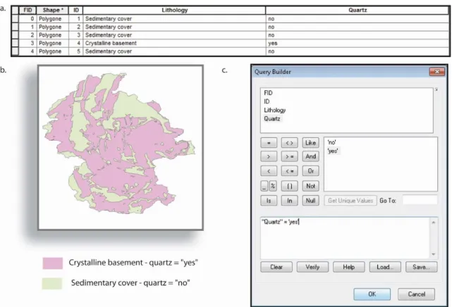
485 Second, the TCN approach assumes a uniform concentration of quartz throughout the
486 catchment area which may bias the results toward the quartz-bearing locations. If instead the
487 quartz content of eroded lithologies varies across the studied basin, equation (4) is no longer
488 valid. However, though it remains relatively difficult to quantify the concentration of quartz from
489 each eroded lithology, we can at least exclude any lithology without quartz from the calculation
490 (e.g. Delunel et al., 2010). We therefore integrated and built an additional option that allows the
491 corresponding area to be removed from the studied watershed.
3 4 5 6 7 8 9 10 11 12 13 14 15 16 17 18 19 20 21 22 23 24 25 26 27 28 29 30 31 32 33 34 35 36 37 38 39 40 41 42 43 44 45 46 47 48 49 50 51 52 53 54 55
For Peer Review
492 Third, the presence of an ice cap may shield the ground surface from incoming cosmic
493 rays, thereby reducing or preventing cosmogenic in situ production. Basinga also allows a
494 correction for ice cover when computing the scaling factor and cosmogenic production rate. We
495 assume that the ice cover is sufficiently thick to fully shield the surface and thus that no
496 cosmogenic isotopes are produced below the ice (Wittmann et al., 2007). However, because ice
497 erosion remains efficient, the area covered by ice may still deliver sediment to the main stream
498 (Wittmann et al., 2007). As they have previously been shielded by ice, in Basinga these
499 sediments are presumed to be free of cosmogenic isotopes. However, in nature, processes of
500 glacial erosion are far more complex, with notably, supra-glacial hillslopes providing sediments
501 whose cosmogenic concentration may differ from 0 (e.g. Godard et al., 2012; Guillon et al.,
502 2015). Moreover, the ice cover may have varied during time with periods of retreat and hence
503 cosmic exposition and periods of advance and shielding. Accounting for all these glacial
504 complexities in order to calculate more accurate denudation rates is likely vain. Therefore, the
505 goal of this new option is not to improve the precision of the denudation rates but to provide
end-506 member values of the denudation rates. Indeed, because glaciers are located at high elevations,
507 assuming a zero production under the ice could result in an underestimation of production rates
508 and thus an underestimation of the true denudation rates. Conversely, assuming full production
509 by ignoring the ice cap would lead to overestimation of the production and denudation rates. The
510 two scenarios can be easily tested using Basinga to bracket the true denudation rates.
511 Like glacial cover, snow cover can also partially shield the rocks and should be accounted
512 for when estimating the production rates. This effect is particularly significant in high elevation
513 mountain ranges, and may induce a reduction of the overall production rate by 5 to 10% (Scherler
514 et al., 2014; Schildgen et al., 2005). Schildgen et al. (2005) attempted to correct for snow cover
515 using a complex physical model coupled with remote sensing monitoring of snow cover spanning
516 several years, which required calibration from ground-based records and measurements. Snow
517 thickness can also be estimated from Precipitation Daily Data (PDD) derived from Global
518 Climate Models (GCM). Such calculations are far beyond the goal of Basinga. However, this
519 correction can be computed independently and integrated into Basinga by multiplying it by the
520 topographic shielding factor. In such a case, the snow correction will be included in the overall
521 calculation if the correction for topographic shielding is selected during the process.
522 3 4 5 6 7 8 9 10 11 12 13 14 15 16 17 18 19 20 21 22 23 24 25 26 27 28 29 30 31 32 33 34 35 36 37 38 39 40 41 42 43 44 45 46 47 48 49 50 51 52 53 54 55
For Peer Review
523 5.7 Estimation of the denudation uncertainties524 Basinga also provides an estimation of the denudation uncertainties. However, errors in 525 the cosmogenic production rates and the measured concentrations are only propagated as follows:
526 527 𝛿𝜀 =
[
𝛿𝑁𝑁2(
𝑃𝑠𝑝𝑎𝑙 𝜌 Λ𝑛,𝑟𝑜𝑐𝑘 + 𝑃𝑠𝑚𝜌 Λ𝜇 𝑠𝑚, 𝑟𝑜𝑐𝑘 + 𝑃𝑓𝑚𝜌 Λ𝜇 𝑓𝑚, 𝑟𝑜𝑐𝑘)
]
2 +(
𝑃𝑠𝑝𝑎𝑙 . 𝛿𝑃𝑠𝑝𝑎𝑙𝑁 𝜌 Λ𝑛,𝑟𝑜𝑐𝑘)
2 +(
𝑃𝑠𝑚 . 𝛿𝑃𝑠𝑚 𝑁𝜌 Λ𝜇 𝑠𝑚, 𝑟𝑜𝑐𝑘)
2 +(
𝑃𝑓𝑚 . 𝛿𝑃𝑓𝑚 𝑁𝜌 Λ𝜇 𝑓𝑚, 𝑟𝑜𝑐𝑘)
2 528 (13) 529530 where N, N and are the measured concentration of the studied nuclide, its 1 uncertainty, and 𝜀
531 the error in the denudation rates, respectively. Pi represents the uncertainty in the cosmogenic
532 production rates for spallation and muons. Basinga attaches, to the spallogenic production
533 parameters, the uncertainties provided in Martin et al. (2017) as a function of the studied nuclide,
534 the scaling model and the ERA40 database (see table 7 of Martin et al. (2017). This represents,
535 on average, an uncertainty of less than 10%, consistent with the value proposed in Balco et al.
536 (2008). This uncertainty accounts for variability resulting from both these production rate
537 calibrations and from the spatial scaling (Balco et al., 2008). We attached a value of 20% for
538 both muogenic production uncertainties based on the standard deviation of the surficial SLHL
539 estimate of Braucher et al. (2013). All these values can be easily changed and updated if needed
540 (see online supplementary information).
541 A more rigorous approach would consider all of the parameters in equation 4 and their
542 related uncertainties but would require a laborious partial derivation. This error propagation could
543 also be performed using a numerical approach based on a Monte Carlo simulation that explores
544 the range of all the input parameters (Puchol et al., 2017). Such an approach would require
545 further developments that are beyond the scope of the present tool.
546
547 7. Conclusion
548 Our sensitivity analysis suggests that inverting denudation rates from the cosmogenic
549 concentration measured at the basin outlet using the analytical approach, which assumes constant
550 attenuation lengths of muons in the rocks and spatially variable denudation rates, remains as
551 accurate as the second, more sophisticated, iterative approach. The attenuation lengths of muons
552 have little impact on the final denudation rates determined whatever the latitude, denudation and
3 4 5 6 7 8 9 10 11 12 13 14 15 16 17 18 19 20 21 22 23 24 25 26 27 28 29 30 31 32 33 34 35 36 37 38 39 40 41 42 43 44 45 46 47 48 49 50 51 52 53 54 55
For Peer Review
553 relief of the studied basin. The analytical approach is moreover computationally more rapid and
554 does not require the relatively unrealistic hypothesis that denudation rates are homogenous
555 throughout the studied basins.
556 Consequently, Basinga is based on these results and calculates the denudation rates using
557 the analytical approach (method 2). However, this method neglects past variations in the Earth’s
558 magnetic field. To address this issue, through Basinga we developed a new simplified approach
559 for correcting for paleomagnetic changes. This approach is based on integration of the production
560 rates during the equivalent exposure time, which is approximated at the basin scale by dividing
561 the present-day basin-average production rates by the cosmogenic concentration measured at the
562 outlet.
563 Our analysis also shows that the choice of the scaling model may be critical in some
564 regions where the Lal/Stone and LSD factors can differ by up to 30% leading to large
565 discrepancies in the denudation results. Because calibration data are sparse in many regions of the
566 world, it is difficult to determine which of the two models is the most accurate. New calibration
567 data sites are therefore needed, especially in regions where the scaling factors determined by two
568 schemes differ strongly. Until such data are made available, in regions of low relief with a strong
569 difference between the two models, both models should be used in the calculation to provide a
570 range of possible denudation values. Consequently, the two models are available in Basinga.
571 However, calculation of scaling factors using the LSD model is computationally longer, which
572 precludes application of this model to a large dataset. To overcome this limitation, we developed
573 in Basinga an alternative approach in which the LSD factors are interpolated for the whole basin
574 from the Lal/Stone factors. This interpolation is based on a polynomial law that is fitted using a
575 limited number of cells in which both models have been used to calculate scaling factors.
576 Basinga is a freely available GIS toolbox that provides two independent tools for 577 computing basin average cosmogenic scaling factors, cosmogenic 10Be, 3He and 21Ne production 578 rates, and associated denudation rates, from the cosmogenic concentrations. It presents several
579 significant improvements with respect to the literature:
580 (1) it is based on user-friendly interfaces, for which comprehensive instructions and help are
581 provided. Its use does not require any particular skills in programming.
3 4 5 6 7 8 9 10 11 12 13 14 15 16 17 18 19 20 21 22 23 24 25 26 27 28 29 30 31 32 33 34 35 36 37 38 39 40 41 42 43 44 45 46 47 48 49 50 51 52 53 54 55
For Peer Review
582 (2) it can be run on either ArcGIS or QGIS. It is therefore the first existing tool which couples a
583 code-based program to calculate the cosmogenic production and denudation rates with the
584 powerful skills of a GIS system.
585 (3) it computes the scaling factors and cosmogenic rates in a few minutes for several catchments
586 together and allows quick processing of large datasets.
587 (4) it is the first existing tool which calculates the LSD scaling factors at the basin scale
588 (5) it is the first tool that provides, at the basin scale, a correction for paleomagnetic changes, ice
589 cover and geology.
590 Basinga can be easily downloaded from the Online Supplementary Information and installed 591 following the instructions "Getting Started" document, also provided online. The
592 parameterization can be easily updated or changed if needed following the instructions given in
593 the "Getting Started" document.
594
595 Acknowledgements
596 We thank Jérôme Lavé and Maarten Lupker for fruitful discussions about cosmogenic nuclides
597 and denudation rates. We also thank Pauline Collon and Christine Fay-Varnier for their
598 assistance and help with programing in Python. We are also thankful to the associate editor and
599 two anonymous reviewers for their reading and comments which greatly improved the quality of
600 this manuscript. We dedicate this work to the fictional, but Nobel-Prize-worthy Sheldon Cooper,
601 from Caltech, who greatly inspired the name of our tool. This is CRPG contribution 2692.
602 603
604 References
605 Balco, G., 2017. Production rate calculations for cosmic-ray-muon-produced 10Be and 26Al
606 benchmarked against geological calibration data. Quat. Geochronol. 39, 150–173.
607 doi:10.1016/j.quageo.2017.02.001
608 Balco, G., Briner, J., Finkel, R.C., Rayburn, J.A., Ridge, J.C., Schaefer, J.M., 2009. Regional
609 beryllium-10 production rate calibration for late-glacial northeastern North America. Quat.
610 Geochronol. 4, 93–107. doi:10.1016/j.quageo.2008.09.001
611 Balco, G., Stone, J.O., Lifton, N.A., Dunai, T.J., 2008. A complete and easily accessible means of
612 calculating surface exposure ages or erosion rates from 10Be and 26Al measurements. Quat.
3 4 5 6 7 8 9 10 11 12 13 14 15 16 17 18 19 20 21 22 23 24 25 26 27 28 29 30 31 32 33 34 35 36 37 38 39 40 41 42 43 44 45 46 47 48 49 50 51 52 53 54 55
For Peer Review
613 Geochronol. 3, 174–195. doi:10.1016/j.quageo.2007.12.001614 Bierman, P., Steig, E.J., 1996. ESTIMATING RATES OF DENUDATION USING
615 COSMOGENIC ISOTOPE ABUNDANCES IN SEDIMENT. Earth Surf. Process.
616 Landforms 21, 125–139.
617 Borchers, B., Marrero, S., Balco, G., Caffee, M., 2015. Geological Calibration of Spallation
618 Production Rates in the CRONUS-Earth Project.
619 Braucher, R., Bourlès, D., Merchel, S., Vidal Romani, J., Fernadez-Mosquera, D., Marti, K.,
620 Léanni, L., Chauvet, F., Arnold, M., Auma??tre, G., Keddadouche, K., 2013. Determination
621 of muon attenuation lengths in depth profiles from in situ produced cosmogenic nuclides.
622 Nucl. Instruments Methods Phys. Res. Sect. B Beam Interact. with Mater. Atoms 294, 484–
623 490. doi:10.1016/j.nimb.2012.05.023
624 Braucher, R., Merchel, S., Borgomano, J., Bourlès, D.L., 2011. Production of cosmogenic
625 radionuclides at great depth : A multi element approach. Earth Planet. Sci. Lett. 309, 1–9.
626 doi:10.1016/j.epsl.2011.06.036
627 Brown, E.T.., Stallard, R.F., Larsen, M.C., Raisbeck, G.M., Yiou, F., 1995. Denudation rates
628 determined from the accumulation of in situ-produced 10Be in the Luquillo Experimental
629 Forest, Puerto Rico. Earth Planet. Sci. Lett. 129, 193–202.
630 Carretier, S., Regard, V., Vassallo, R., Aguilar, G., Martinod, J., Riquelme, R., Christophoul, F.,
631 Charrier, R., Gayer, E., Farías, M., Audin, L., Lagane, C., 2015. Differences in 10Be
632 concentrations between river sand, gravel and pebbles along the western side of the central
633 Andes. Quat. Geochronol. 27, 33–51. doi:10.1016/j.quageo.2014.12.002
634 Charreau, J., Blard, P.H., Puchol, N., Avouac, J.P., Lallier-Vergès, E., Bourlès, D., Braucher, R.,
635 Gallaud, A., Finkel, R., Jolivet, M., Chen, Y., Roy, P., 2011. Paleo-erosion rates in Central
636 Asia since 9Ma: A transient increase at the onset of Quaternary glaciations? Earth Planet.
637 Sci. Lett. 304, 85–92. doi:10.1016/j.epsl.2011.01.018
638 Chmeleff, J., von Blanckenburg, F., Kossert, K., Jakob, D., 2010. Determination of the 10Be
639 half-life by multicollector ICP-MS and liquid scintillation counting. Nucl. Instruments
640 Methods Phys. Res. Sect. B Beam Interact. with Mater. Atoms 268, 192–199.
641 Danielson, J.J., Gesch, D.B., 2011. Global Multi-resolution Terrain Elevation Data 2010. U.S.
642 Geol. Surv. Open-File Rep. 2011 1073, 26 p.
643 Delunel, R., van der Beek, P.A., Carcaillet, J., Bourlès, D.L., Valla, P.G., 2010. Frost-cracking
3 4 5 6 7 8 9 10 11 12 13 14 15 16 17 18 19 20 21 22 23 24 25 26 27 28 29 30 31 32 33 34 35 36 37 38 39 40 41 42 43 44 45 46 47 48 49 50 51 52 53 54 55
For Peer Review
644 control on catchment denudation rates: Insights from in situ produced 10Be concentrations
645 in stream sediments (Ecrins–Pelvoux massif, French Western Alps). Earth Planet. Sci. Lett.
646 293, 72–83. doi:10.1016/j.epsl.2010.02.020
647 Derrieux, F., Siame, L.L., Bourlès, D.L., Chen, R., Braucher, R., Léanni, L., Lee, J., Chu, H.,
648 Byrne, T.B., 2014. How fast is the denudation of the Taiwan mountain belt ? Perspectives
649 from in situ cosmogenic 10 Be. J. Asian Earth Sci. 88, 230–245.
650 doi:10.1016/j.jseaes.2014.03.012
651 Desilets, D., Zreda, M., Prabu, T., 2006. Extended scaling factors for in situ cosmogenic
652 nuclides: New measurements at low latitude. Earth Planet. Sci. Lett. 246, 265–276.
653 Dibiase, R.A., 2018. Increasing vertical attenuation length of cosmogenic nuclide production on
654 steep slopes negates topographic shielding corrections for catchment erosion rates. Earth
655 Surf. Dyn. Discuss. 1–17.
656 Dunai, T.J., 2001. Influence of secular variation of the geomagnetic field on production rates of
657 in situ produced cosmogenic nuclides. Earth Planet. Sci. Lett. 193, 197–212.
658 Dymond, J.R., Betts, H.D., Schierlitz, C.S., 2010. An erosion model for evaluating regional
land-659 use scenarios. Environ. Model. Softw. 25, 289–298. doi:10.1016/j.envsoft.2009.09.011
660 Fox, M., Leith, K., Bodin, T., Balco, G., Shuster, D.L., 2015. Rate of fluvial incision in the
661 Central Alps constrained through joint inversion of detrital 10 Be and thermochronometric
662 data. Earth Planet. Sci. Lett. 411, 27–36. doi:10.1016/j.epsl.2014.11.038
663 Godard, V., Bourles, D.L., Spinabella, F., Burbank, D.W., Bookhagen, B., Fisher, G.B., Moulin,
664 A., Leanni, L., 2014. Dominance of tectonics over climate in Himalayan denudation.
665 Geology 42, 243–246. doi:10.1130/G35342.1
666 Godard, V., Burbank, D.W., Bourlès, D.L., Bookhagen, B., Braucher, R., Fisher, G.B., 2012.
667 Impact of glacial erosion on 10 Be concentrations in fluvial sediments of the Marsyandi 668 catchment, central Nepal. J. Geophys. Res. 117, F03013. doi:10.1029/2011JF002230
669 Gosse, J.C., Phillips, F.M., 2001. Terrestrial in situ cosmogenic nuclides: theory and application.
670 Quat. Sci. Rev. 20, 1475–1560.
671 Guillon, H., Mugnier, J., Buoncristiani, J., Carcaillet, J., Godon, C., Beek, P. Van Der, Vassallo,
672 R., 2015. Improved discrimination of subglacial and periglacial erosion using 10 Be
673 concentration measurements in subglacial and supraglacial sediment load of the Bossons
674 glacier ( Mont Blanc massif , France ) 1215, 1202–1215. doi:10.1002/esp.3713
3 4 5 6 7 8 9 10 11 12 13 14 15 16 17 18 19 20 21 22 23 24 25 26 27 28 29 30 31 32 33 34 35 36 37 38 39 40 41 42 43 44 45 46 47 48 49 50 51 52 53 54 55