Detailed validation of the bidirectional effect in various Case 1 waters for application to ocean color imagery

(1)

HAL Id: hal-00330326

https://hal.archives-ouvertes.fr/hal-00330326

Submitted on 26 Sep 2007

HAL is a multi-disciplinary open access

archive for the deposit and dissemination of

sci-entific research documents, whether they are

pub-lished or not. The documents may come from

teaching and research institutions in France or

abroad, or from public or private research centers.

L’archive ouverte pluridisciplinaire HAL, est

destinée au dépôt et à la diffusion de documents

scientifiques de niveau recherche, publiés ou non,

émanant des établissements d’enseignement et de

recherche français ou étrangers, des laboratoires

publics ou privés.

Detailed validation of the bidirectional effect in various

Case 1 waters for application to ocean color imagery

K. J. Voss, A. Morel, David Antoine

To cite this version:

K. J. Voss, A. Morel, David Antoine. Detailed validation of the bidirectional effect in various Case 1

waters for application to ocean color imagery. Biogeosciences, European Geosciences Union, 2007, 4

(5), pp.781-789. �hal-00330326�

(2)

www.biogeosciences.net/4/781/2007/ © Author(s) 2007. This work is licensed under a Creative Commons License.

Biogeosciences

Detailed validation of the bidirectional effect in various Case 1

waters for application to ocean color imagery

K. J. Voss1, A. Morel2, and D. Antoine2

1_{Department of Physics, University of Miami, Coral Gables, Florida, USA}

2_{Laboratoire d’Oc´eanographie de Villefranche, Universit´e Pierre et Marie Curie et Centre National de la Recherche} Scientifique, Villefranche-sur-mer, France

Received: 7 June 2007 – Published in Biogeosciences Discuss.: 27 June 2007

Revised: 17 September 2007 – Accepted: 17 September 2007 – Published: 26 September 2007

Abstract. The radiance viewed from the ocean depends on

the illumination and viewing geometry along with the wa-ter properties, and this variation is called the bidirectional effect. This bidirectional effect depends on the inherent op-tical properties of the water, including the volume scattering function, and is important when comparing data from differ-ent satellite sensors. The currdiffer-ent model of f/Q, which con-tains the bidirectional effect, by Morel et al. (2002) depends on modeled, not measured, water parameters, thus must be carefully validated. In this paper we combined upwelling ra-diance distribution data from several cruises, in varied water types and with a wide range of solar zenith angles. We com-pared modeled and measured Lview/Lnadirand found that the average difference between the model and data was less than 0.01, while the RMS difference between the model and data was on the order of 0.02–0.03. This is well within the statis-tical noise of the data, which was on the order of 0.04–0.05, due to environmental noise sources such as wave focusing.

1 Introduction

The upwelling radiance distributions, either beneath the in-terface or emerging from the water, are not isotropic, but vary with illumination and viewing conditions and also with water optical properties. Knowing how to predict this angular vari-ation is important in satellite oceanography, as the analysis of satellite derived upwelling radiances must take into account these variations. This is particularly important when compar-ing different ocean color sensors as these sensors will view the same spot at different times (hence varied illumination geometry) and under different view angles. One must have a model of this variation of the radiance distribution that is dependent on a small set of parameters, but which can

accu-Correspondence to: K. J. Voss

(voss@physics.miami.edu)

rately predict the variation. As the available model for Case I waters (Morel et al., 2002) is based on radiation transport computations, it is essentially theoretical in nature. More-over, it includes assumptions and parameterizations of the inherent optical properties, as a function of the chlorophyll concentration, which presently are not fully verified (this is particularly true for the volume scattering function). There-fore a comparison between field data and model predictions over a wide range of experimental conditions is necessary. This is the objective of the present paper which makes use of recent and numerous observations in the Pacific Ocean and in the Mediterranean Sea.

The shape of the upwelling radiance distribution,

Lu(θ0, θv, φ), can be described by the bidirectional function,

denoted Q(θo, θv, φv), which is defined as:

Q(θo, θv, φv) = Eu/Lu(θo, θv, φv) (1)

where θois the solar zenith angle, θvis the view nadir angle,

φ is the azimuth between these two directions, and Euis the

planar upward irradiance, i.e., the integral of the upward radi-ance field over the half space (2π sr). The Morel et al. (2002) model, which is commonly used in satellite oceanography, characterizes the variations in Q as a function of the three angles and of the chlorophyll concentration, [Chl]. [Chl] is a convenient index for Case 1 waters as it characterizes the bio-optical state of the water bodies. This model incorpo-rates both a correction for this varying Q factor, and also a correction for the f factor. The f factor relates the irradiance reflectance to the absorption coefficient and the backscatter-ing coefficient, a and bb, respectively, through

R(λ) = f (λ)[bb(λ)/a(λ)]. (2)

where f (λ) for a given water is also dependent on the solar zenith angle.

This paper will describe our results in validating the Q factor. The problem of validating f could be addressed with irradiance reflectance measurements combined with bb and

(3)

782 K. J. Voss et al.: Validation of BRDF in Case 1 waters

Fig. 1. Data distribution in terms of [Chl] and solar zenith angle.

a measurements, but we do not have a large database of

con-temporaneous bband a coefficients for such a validation.

In the past we have had two investigations looking at the accuracy of the series of Q values as predicted by models (Morel et al., 1995; Voss and Morel, 2005). Each of these was done with a different version of our radiance distribu-tion camera systems (RADS: Voss, 1989; RADS-II, Voss and Chapin, 1992). These early instruments were large and slow and provided a limited data set. Recently we have devel-oped a new generation of radiance distribution camera sys-tems specifically aimed at looking at the upwelling radiance distribution (NuRADS: Voss and Chapin, 2005). With this new instrument we have an extensive set of upwelling radi-ance distribution data in both Case I and Case II waters. This paper will concentrate on the Case I waters, as this is where the 2002- model was designed to work. The Case II situation is much more complicated, less predictable (e.g. Loisel and Morel, 2001), and will be separately addressed in later work. The first investigation (1995) was carried out off of Cal-ifornia with a stable [Chl] value (0.3 mg m−3_{), and widely} varying sun zenith angle (32◦_{to 80}◦_{). In contrast, the second}

investigation (2005), with measurements around the Baja Peninsula, encompassed a large range of chlorophyll con-centrations ([Chl] from 0.14 to 11 mg m−3), whereas the sun

angle remained in a rather restricted range (28◦to 40◦). Al-though these validations were successful, it is still highly desirable to test the quality of the predictions over a larger variety of situations, regarding both the trophic state of the waters and the illumination conditions. In the present study, we will specifically concentrate on two cruises, in the South Pacific and Mediterranean Sea, and several short cruises near Hawaii, which together offer such a variety of situations.

During the BIOSOPE cruise in the South Pacific, ex-tremely clear oligotrophic waters ([Chl]<0.03 mg m−3), as

well as moderately eutrophic waters inside the Chilean up-welling zone ([Chl]>1.4 mg m−3) were encountered. The

AOPEX cruise took place in the Mediterranean, and while the water types were not as varied ([Chl]∼0.07 to 0.15 mg m−3), we had the opportunity to sample the radiance

distribution for a variety of solar zenith angles. In addition to these two cruises, we have an extensive set of radiance dis-tribution measurements in clear waters around Hawaii ([Chl] approximately 0.1 mg m−3). All of the radiance distribution

measurements were done with the camera just below the sur-face (at approximately 0.75 m).

2 Data set description

The distribution of the data set is best described by Fig. 1 that illustrates the range of [Chl] and solar zenith angle for the ra-diance distribution data presented in this paper. The Hawaii data set has points in the [Chl] range below 0.2 mg m−3, but has a large range of solar zenith angles, from almost 0◦ to over 70◦. The AOPEX data is over a similar [Chl] range (<0.2 mg m−3) but a slightly more limited solar zenith

angle range (20◦<θo<75◦). The BIOSOPE data from the

South Pacific has the wider [Chl] range, from <0.05 to

>1.4 mg m−3, and θo from 10◦ to 60◦. The entire data set,

however, does have a large hole in the 0.4 to 1.0 mg m−3 range.

For the AOPEX and BIOSOPE cruises, the chlorophyll concentration was determined via High-Performance Liquid Chromatography (HPLC), according to a slightly modified version (see Ras et al., 2007) of the method initiated by Van Heukelen and Thomas (2001). The simplified notation [Chl] actually represents the sum of the concentrations of the fol-lowing suite of pigments: chlorophyll a, divinyl chlorophyll a, chlorophyllid a, and chlorophyll a allomers and epimers.

The upward radiance data set was obtained using the Nu-RADS camera system, that has been described in detail pre-viously (Voss and Chapin, 2005). The important details are that it has an automatic filter changer, with positions for 6 spectral filters, a cooled CCD camera, and a fisheye lens to capture the complete upwelling hemisphere of data. In this paper we will use only 4 of these filters: 412, 436, 486, 526 nm. The other 2 filters are at longer wavelengths, and there is appreciable instrument self-shadowing even in clear water. In the configuration used in most of these cruises, floatation is attached to the back of the camera, and the in-strument can be floated away from the ship at a distance ex-ceeding 50 m, to avoid ship shadow, and tethered to the ship using a neutrally buoyant cable which combines power and communication. A portion of the data set was obtained with this system, while another portion was obtained while the instrument was in the configuration shown in Fig. 2. The system can automatically cycle through the spectral filters and collect data that are stored on the internal hard drive. It takes approximately 2 min to obtain a complete set of spec-tral data, and the instrument typically is set to continually cycle and collect multiple sets of radiance distribution data at each wavelength.

(4)

Fig. 2. Illustrating NuRads in its deployment configuration. The

instrument can be floated away from the ship, suspended on the floats just below the surface.

3 Data reduction

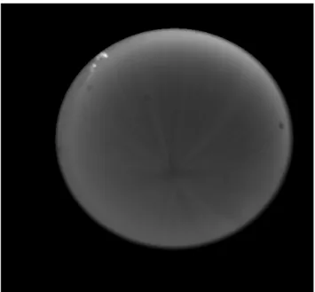
Pre- and post-calibrations were done on the instruments for each cruise. The overall process to calibrate these systems is described in Voss and Zibordi (1989). An additional calibra-tion step has been found to be required which accounts for the immersion of the dome window used in the system and its affect on the throughput of the optical system (immersion factor). This calibration step is briefly described in Voss and Chapin (2005). Images from the system have the calibration applied and result in a fisheye projection image of the up-welling radiance distribution. An example image is shown in Fig. 3.

The NuRADS instrument obtains a complete spectral set of data every 2 min. However, since the whole upwelling ra-diance distribution is obtained very quickly (less than 1 s), individual images often have strong features, such as wave focusing (seen in Fig. 3) , which need to be averaged out. During the data reduction process we look at each image and determine, manually, where the anti-solar point is lo-cated. This point is obvious as it is the point where the wave focused light rays converge. Once this point has been de-termined, a computer program determines where the nadir point should be. This process uses the known angular dis-tance between the anti-solar point and nadir, and looks for symmetry around the principal plane (plane containing the nadir and anti-solar point). When the geometry (nadir and anti-solar point in each image) has been determined, we av-erage images taken within 10 min. Since the image should be symmetric around the principal plane, we average each half of the image together. For the data presented in this paper, we exclude data for which only one image (both halves) are averaged, so each data point effectively represents the aver-age of between 4 and 10 separate imaver-age halves. Imaver-ages are

Fig. 3. Example upwelling radiance distribution image. This

ex-ample is from the AOPEX cruise, on 11/8/2004. Solar zenith angle is 35◦, [Chl]=0.1 mg m−3, wavelength is 526 nm. The geometry of this image is such that the nadir point is the center of the circle, the projection places nadir angle as directly related to the radius from the center. The edge of the circle is a nadir angle of 90◦. The anti-solar point is visible in the lower portion of the circle, defined as where the sun rays (the star pattern) converge. The azimuthal di-rection towards the sun is at the top of the image. The dark circles in the image are artifacts of the optical system and are masked out during the averaging process, while the bright part at the top left is probably a small portion of cable.

excluded if there is contamination in anyway (cables float-ing into view for example) or the anti-solar point can not be determined (most often because of clouds). In addition, to further reduce noise, each data point from each image is an average of a 3×3 pixel area (each pixel represents an angu-lar change of approximately 0.4 degrees). An example after this data processing, for the image set containing the image shown in Fig. 3, is shown in Fig. 4.

It is important to understand that there is still environmen-tal noise left in these images. A portion of this noise may be from our instrument system, however this is dominated by effects due to wave focusing, small scale inhomogenities in the water column, and other natural sources. To illustrate how large these variations can be we collect the σ of each data point averaged, i.e.

σ = q_X

(x − ¯x)2_/N._x,_¯ ₍₃₎ where x is a specific pixel value in radiance units (not nor-malized), and ¯x is the average radiance for that view

geom-etry. N is the number of pixels averaged, which is 9 pix-els/image half times the number of image halves, thus be-tween 36 and 90 pixels. Figure 5 shows σ of the average

(5)

784 K. J. Voss et al.: Validation of BRDF in Case 1 waters 80 60 40 20 0 2.0 1.5 1.0 0.5 0.0

Fig. 4. AOPEX data set, solar zenith angle approximately 35◦, data shown in µW cm−2sr−1nm−1. This is an average of 4 images, so each point represents 8 realizations of the radiance distribution. Here Lnadiris 0.64 µW cm−2sr−1nm−1, Qnis 3.72 sr and µu, the

upwelling average cosine, is 0.44. One can see that the wave focus-ing has been averaged out through this process. In this projection the anti-solar point is towards the right of the image along the x-axis. The direction towards the sun is on the left side of the image. Nadir is represented along the x-axis in the center of the semicir-cle. The nadir angle is proportional to the radial distance from the center; data exists out to 90 degrees, or the horizon.

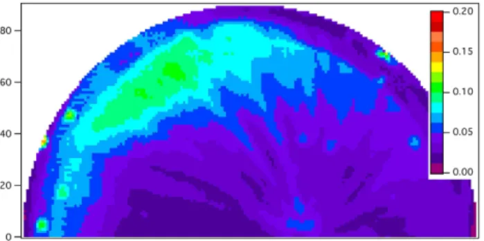
Fig. 5. σ for each data point, in the same projection as Fig. 4. As

can be seen σ can range >0.1 in some areas.

shown in Fig. 4. As can be seen σ shows the effect of wave focusing directly through the apparent sun-rays in this image. However the area with the largest σ is towards the horizon. Figure 6 shows a histogram of σ for one of these averages. As can be seen the peak in the histogram is on the order of 0.03, which limits how well the data could agree with even the best model for individual points.

Any instrument, placed in the water, will have systematic measurement errors due to instrument self-shadowing. For this paper we estimated the effect of self-shadowing follow-ing a variation of the algorithm of Gordon and Dfollow-ing (1992). This algorithm assumes that the shadowing is only propor-tional to the absorption coefficient of the water and the view-ing pathlength that is directly shadowed by the instrument. The original Gordon and Ding (1992) algorithm had a simple disk casting the shadow, we extended this to a three dimen-sional object, with the dimensions of NuRADS, and calcu-lated the shadowlength taking into account the refracted

so-1000 800 600 400 200 0 N um be r of O cc ura nc es (i n 0.002 bi ns ) 0.14 0.12 0.10 0.08 0.06 0.04 0.02 0.00 σ

Fig. 6. Histogram of σ of the individual data points used in above

comparison with the model.

lar zenith angle, view angle, and absorption coefficient. The absorption coefficient was derived from the measured [Chl] using the model of Morel and Maritorena (2001). Because this model is a simple approximation, we only used data for which the shadowing correction was less than 5%. It is possi-ble to derive a more complete correction for shadowing (e.g. Helliwell et al. (1990) and Leathers et al. (2001)), however for radiance distribution measurements, such as these, com-plete knowledge of the seawater volume scattering function (VSF) is required. While we could use the VSF used in the model, this would influence the independence of our com-parison with the data.

Our comparison will be between Lview/Lnadirfor the data and those predicted by the Morel et al. (2002) model and associated tables. According to Eq. (1), the ratio of a slant upward radiance to the nadir radiance is the inverse ratio of the corresponding Q-quantities, so

Lu(θo, θv, φv)/Lu(θo, θv=0, φv=0) = Qn/Q(θo, θv, φv) (4)

here the quantity Qn represents the particular value for the

nadir direction, i.e., Q(θo, θv=0, φv=0), which still depends

on the sun position.

We use the quasi-contemporaneous [Chl] determinations, together with the specific illumination geometry, as deter-mined by the instant of measurement, to enter into the Q-tables.

4 Results

Typical results are shown in Fig. 7 for one day during the BIOSOPE cruise (Station 17, 1/12/2004). Lview/Lnadir for the data and model are displayed, and each data point repre-sents a different direction or data set in that day. The reso-lution of direction is every 5 degrees in nadir and 15 degrees in Azimuth, thus there can be approximately 8 (5–40 degrees in nadir angle) × 12 (0–180 degrees in azimuth angle) = 96 points from each radiance distribution data set. Note that the

(6)

1.20 1.15 1.10 1.05 1.00 0.95 0.90

M

ode

l

L

v ie w

/L

nadi r 1.20 1.15 1.10 1.05 1.00 0.95 0.90

Data L

view

/L

nadir

(a)

1.20 1.15 1.10 1.05 1.00 0.95 0.90

M

ode

l

L

v ie w

/L

nadi r 1.20 1.15 1.10 1.05 1.00 0.95 0.90

Data L

_view

/L

_nadir

(b)

1.20 1.15 1.10 1.05 1.00 0.95 0.90

M

ode

l L

vi

e

w

/L

na

di

r

1.20 1.15 1.10 1.05 1.00 0.95 0.90

Data Lview/Lnadir

(c)

Fig. 7. Graph of model vs data of the ratio Lview/Lnadir for the BIOSOPE Station # 17;[Chl] was 0.11 mg m−3in the upper layer.

(a) 412 nm, (b) 436 nm, and (c) 486 nm. The 1:1 line is also shown.

nadir angle is limited to upward radiances inside the Snell cone, able to emerge from the sea after refraction. For each day we calculated the deviation between the model and data in two ways, first the average difference was determined by:

Difference =X(data−model)/N , (5)

and the RMS was determined by:

RMS=

q_X

(data−model)2_{/N .} ₍₆₎ Through our data set we can look at these factors as a func-tion of [Chl] and solar zenith angle to see if there are any biases in the model. Figures 8a–d shows this for the 4 wave-lengths. In these figures the red dots correspond to the av-erage difference (Eq. 5) while the bars correspond to 1 std

4

2

0 -2

-4

D

iffe

re

nc

e

3 4 5 6 7

0.1

2 3 4 5 6 7

1 Chl

(a)

4

2

0 -2

-4

D

iffe

re

nc

e

3 4 5 6 7

0.1

2 3 4 5 6 7

1 Chl

(b)

6

4

2

0 -2

-4

D

iffe

re

nc

e

3 4 5 6 7

0.1

2 3 4 5 6 7

1 Chl

(c)

6

4

2

0 -2

-4

D

iffe

re

nc

e

3 4 5 6 7

0.1

2 3 4 5 6 7

1 Chl

(d)

Fig. 8. Comparison for the entire data set between Lview/Lnadir the model and the data. (a) 412 nm, (b) 436 nm, (c) 486 nm, and

(d) 526 nm. The red dots are the average difference in agreement

between the model and the data. The bars on each data point are

±1 std. The blue dots are σ obtained in the image averaging process and represents the environmental noise in the images.

(7)

-4

-2

0

2 D

iffe

re

nc

e

50

40

30

20

10 Minimum Zenith Angle

(a)

-4 -2 0 2

D

iffe

re

nc

e

80 70 60 50 40 30 20

Maximum Zenith Angle

(b)

Fig. 9. Difference between the model and data Lview/Lnadir, shown as a function of solar zenith angle. Average difference is shown as red dots, bars are ±1 standard deviation. (a) Maximum solar zenith angle during that data collection, (b) Minimum solar zenith angle during that data collection. As can be seen there is no systematic trend in this difference as a function of solar zenith angle. This example shows the data at 412 nm; there is no significant trend at any of the other wavelengths.

(Eq. 6). While collecting the difference and RMS, we also find the average σ for the data (effectively the average of Fig. 5, for each data point). This gives a measure of the en-vironmental noise for that point, and is shown as the blue squares.

We can also look to see if there is any bias with respect to solar zenith angle. For each day of data we collected the minimum and maximum solar zenith angle, during the data acquisition. These results are shown in Fig. 9. Figures 8 and 9, taken together, show that in this data set there is no systematic difference with either [Chl] or solar zenith angle. In both cases the average difference is much less than 0.01. This is well within both the standard deviation of the differ-ence between the model and measurement and the σ in the measurement alone. In general the RMS difference between the model and data ranged from 0.01 to 0.04, but was mostly on the order of 0.02–0.03. The largest difference tends to be towards the longer wavelengths where increased shadowing

5.0 4.5 4.0 3.5 3.0 M ode l 5.0 4.5 4.0 3.5 3.0 Data Equation 7 Equation 8

(a)

(b)

(c)

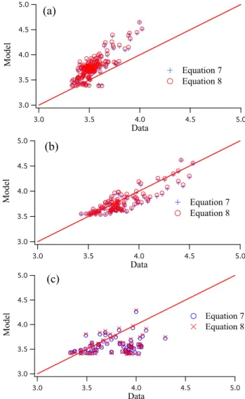
Fig. 10. Aas and Hojerslev (1999) Q_nadir (sr) fit to data set (486 nm). (a) Hawaii data, (b) AOPEX (Mediterranean), (c)

BIOSOPE (South Pacific). As can be seen, the best fit is with the AOPEX data. The 1:1 line is also shown.

may be causing problems in the data.

We can also use this data set to investigate the avail-able models of Qnadir=Q(θo, θv=0,φv=0). Aas and Hojerslev

(1999), using a parameterization based on a dataset from rel-atively clear Mediterranean waters, predicted that Qnadir, at blue (465–475 nm) wavelengths, should follow either:

Qnadir=5.33 exp(−0.45 cos(θo) sr, or (7)

Qnadir=5.20 − 1.82 cos(θo) sr. (8)

Morel et al. (2002) provided an alternate model, which in-cludes a parameter for varying water types given by:

Qnadir(θo, λ, [Chl])=Qo(0, λ, [Chl]) + SQn(λ, [Chl])[1− cos(θo)]

(9)

(8)

5.0 4.5 4.0 3.5 3.0 M ode l 5.0 4.5 4.0 3.5 3.0 Data Hawaii BIOSOPE AOPEX (a) 5.0 4.5 4.0 3.5 3.0 M ode l 5.0 4.5 4.0 3.5 3.0 Data Hawaii BIOSOPE AOPEX (b) 5.0 4.5 4.0 3.5 3.0 M ode l 5.0 4.5 4.0 3.5 3.0 Data Hawaii BIOSOPE AOPEX (c) 5.0 4.5 4.0 3.5 3.0 M ode l 5.0 4.5 4.0 3.5 3.0 Data Hawaii BIOSOPE AOPEX (d)

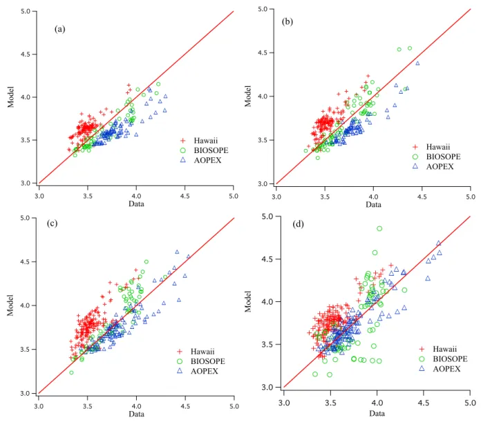
Fig. 11. Comparison of Morel et al. (2002) Qn(sr) model with data set. (a) 412 nm, (b) 436 nm, (c) 486 nm, and (d) 526 nm. The 1:1 line is

also shown.

where Qo(0,λ,[Chl]) and SQn(λ,[Chl]) can be interpolated

from Table 2 in Morel et al. (2002).

The variations in both the initial term, Q0, and the slope,

SQn, with the chlorophyll concentration (used as bio-optical

index) are by far not negligible, and are important when com-paring predictions to actual data obtained in Case 1 waters with various trophic levels.

Figure 10 illustrates how well Eqs. (7) and (8) fit this data set. As can be seen, the best agreement is for the AOPEX data set, which is not surprising as this data set was obtained in the Western Mediterranean Sea, which was where the em-pirical factors in Eqs. (7) and (8) were determined, probably with similar [Chl] values. To quantitatively characterize this fit we calculate the RMS difference between the model and data. The RMS for these fits are 0.24 sr (Hawaii), 0.14 sr

(AOPEX), 0.30 sr (BIOSOPE), and 0.24 sr for the combined data set. This also shows that Eqs. (7) and (8) are very good at fitting the AOPEX data set, and not as good at the other sites. It is obvious that a line fitted between the model and data would be significantly different than 1 for both the Biosope and Hawaii data.

Figure 11 illustrates the fit of Eq. (9) to the data set for the 4 wavelengths. The RMS differences are shown in Table 1. The model fits the data a little better than the earlier model, but there are differences in the individual data sets. Interest-ingly, for most wavelengths, there is a good fit of the model to the BIOSOPE data, that extend over a rather wide range of

Qnadirvalues, in correspondence with the wider [Chl] range encountered during this campaign. However, we did not have [Chl] values approaching 10 mg m−3, thus did not see the

(9)

Table 1. RMS difference between Qn (sr) model (Morel et al.,

2002) and data set.

Wavelength Cruise 412 436 486 526 BIOSOPE 0.11 0.10 0.14 0.17 AOPEX 0.20 0.18 0.12 0.11 Hawaii 0.16 0.19 0.26 0.26 Combined 0.16 0.17 0.21 0.20

predicted maximal Qnadir values (close to 5 steradians) as observed in the Gulf of California (Voss and Morel, 2005).

Zibordi and Berthon (2001) have described an additional model for Qnadirbased on data obtained in the Adriatic Sea, however this water type was significantly different than our data base, hence did not agree very well with our data and is not shown.

5 Conclusions

The comparison between model predictions and field data has been carried out over a wide range of environmental con-ditions with respect to the trophic state of the water and the sun position in clear skies. The bidirectional variation (po-lar and azimuthal angles) of the upward radiance distribu-tion compared to the radiance from nadir direcdistribu-tion, as well as the variation of this particular radiance with the sun an-gle have been successfully tested. The model (Morel et al., 2002) proves to be a very good tool in reproducing the vari-ous radiance distributions that we observed in our extensive data set for Case I waters. However each real, measured, radiance distribution has many features in it due to wave fo-cusing and downwelling illumination variations. As such, while the model is able to accurately predict the average, it will never exactly fit a measured radiance distribution (nor should it be expected to do this). Much more work needs to be done to move this Case I model into the Case II regime. We currently are looking at this Case II situation with 2 data sets collected in the Chesapeake Bay, and are also looking into issues of the polarization of the upwelling light field.

As a practical conclusion, it can be added that the bidirec-tional corrections based on the lookup tables generated from the model, and presently applied to ocean color imagery, is sound and amply validated for Case I waters, i.e., for most parts of the global ocean. The application of such a correc-tion is needed for a meaningful comparison of the normalized water-leaving radiances inside and between various scenes, as well as for a merging of products derived from various sensors.

Acknowledgements. This work was supported by NASA (#NNG04HZ21C to KV). N. Souaidia and A. Chapin were, respectively, instrumental to collecting the BIOSOPE and AOPEX radiance distribution data; J. Ras who made the pigment analyses for both cruises is warmly thanked. The Hawaii data was col-lected in collaboration with D. Clark’s group at NOAA/NESDIS, specifically M. Ondrusek and Yong Sung Kim.

The BIOSOPE and AOPEX projects and cruises were funded by CNRS and INSU (Centre National pour la Recherche Scien-tifique and Institut des Sciences de l’Univers), by the Centre Na-tional d’Etudes Spatiales (CNES), by the European Space Agency (ESA), and by the National Aeronautics and Space Administration (NASA), and, for BIOSOPE (a project of the LEFE-CYBER pro-gram), by the Engineering Research Council of Canada (NSERC). The expertise of the captains, officers and crews of the research vessels Atalante (BIOSOPE) and Suroit (AOPEX) were essential for the success of these campaigns. We thank H. Claustre and A. Sciandra, the chief scientists of the BIOSOPE campaign.

This paper is dedicated to the memory of A. Chapin, a colleague and friend for over 20 years. He was instrumental in the develop-ment of the series of electro-optic radiance distribution cameras, along with many other instruments, and contributed to many experiments at sea during this long period.

Edited by: E. Boss

References

Aas, E. and Hojerslev, N. K.: Analysis of underwater radiance dis-tribution observations: Apparent optical properties and analytical functions describing the angular radiance distributions, J. Geo-phys. Res., 104, 8015–8024, 1999.

Gordon, H. R. and Ding, K.: Self-shading of in-water optical mea-surements, Limnol. Oceanogr., 37, 491–500, 1992.

Helliwell, W. S., Sullivan, G. N., Macdonald, B., and Voss, K. J.: A finite-difference discrete-ordinate solution to the three di-mensional radiative transfer equation, Transport Theor. Stat., 19, 333–356, 1990.

Leathers, R., Downes, T. V., and Mobley, C. Self-shading correc-tion for upwelling sea-surface radiance measurements made with buoyed instruments, Opt. Express, 8, 561–570, 2001.

Loisel, H. and Morel, A.: Non-isotropy of the upward radiance field in typical coastal (Case-2) waters, Int. J. Remote Sens., 22, 275– 295, 2001.

Morel, A., Antoine, D., and Gentili, B.: Bidirectional reflectance of oceanic waters: Accounting for Raman emission and vary-ing particle scattervary-ing phase function, Appl. Opt. 41, 6289–6306, 2002.

Morel, A., and Maritorena, S. Bio-optical properties of oceanic wa-ters: a reappraisal. J. Geophys. Res., 106, 7163–7180, 2001. Morel, A., Voss, K. J., and Gentili, B.: Bi-directional reflectance

of oceanic waters: A comparison of model and experimental re-sults, J. Geophys. Res., 100, 13 143–13 150, 1995.

Ras, J., Uitz, J., and Claustre. H.: Spatial variability of phyto-plankton pigments distribution in the South Eat Pacific, Biogeo-sciences Discuss., accepted, 2007.

Van Heukelen, L. and Thomas, C. S.: Computer-assisted high-performance liquid chromatography method development with

(10)

application to the isolation and analysis of phytoplankton pig-ments, J. Chromatogr., 910, 31–49, 2001.

Voss, K. J.: Electro-optic camera system for measurement of the underwater radiance distribution, Opt. Eng., 28, 241–247, 1989. Voss, K. J. and Chapin, A. L.: Next generation in-water radiance distribution camera system, Proc. Soc. Photo-Optical Instrumen-tation Engineers, 1750, 384–387, 1992.

Voss, K. J. and Chapin, A. L.: Upwelling radiance distribution cam-era system, NURADS, Opt. Express, 13, 4250–4262, 2005.

Voss, K. J. and Morel, A.: Bidirectional reflectance function for oceanic waters with varying chlorophyll concentrations: Mea-surements versus predictions, Limnol. Oceanogr., 50, 698–705, 2005.

Voss, K. J. and Zibordi, G.: Radiometric and geometric calibration of a spectral electro-optic “fisheye” camera radiance distribution system, J. Atmos. Ocean. Techn., 6, 652–662, 1989.

Zibordi, G. and Berthon, J.-F.: Relationships between Q- fac-tor and seawater optical properties in a coastal region, Limnol. Oceanogr., 46, 1130–1140, 2001.