HAL Id: hal-02180642
https://hal.archives-ouvertes.fr/hal-02180642
Submitted on 6 Oct 2020
HAL is a multi-disciplinary open access
archive for the deposit and dissemination of sci-entific research documents, whether they are pub-lished or not. The documents may come from teaching and research institutions in France or abroad, or from public or private research centers.
L’archive ouverte pluridisciplinaire HAL, est destinée au dépôt et à la diffusion de documents scientifiques de niveau recherche, publiés ou non, émanant des établissements d’enseignement et de recherche français ou étrangers, des laboratoires publics ou privés.
Seismic and aseismic moment budget and implication for
the seismic potential of the Parkfield Segment of the San
Andreas Fault
Sylvain Michel, Jean-Philippe Avouac, Romain Jolivet, Lifeng Wang
To cite this version:
Sylvain Michel, Jean-Philippe Avouac, Romain Jolivet, Lifeng Wang. Seismic and aseismic moment budget and implication for the seismic potential of the Parkfield Segment of the San Andreas Fault. Bulletin of the Seismological Society of America, Seismological Society of America, 2018, 108 (1), pp.19-38. �10.1785/0120160290�. �hal-02180642�
1
Seismic and Aseismic Moment Budget and Implication for the Seismic Potential of the
1
Parkfield Segment of the San Andreas Fault.
2 3
Sylvain Michel1, Jean-Philippe Avouac2, Romain Jolivet3 and Lifeng Wang4
4
1University of Cambridge, Department of Earth Sciences, Cambridge, UK
5
2California Institute of Technology, Department of Geology and Planetary Sciences, Pasadena, CA, USA
6
3Laboratoire de Géologie, Département de géosciences, École Normale Supérieure, CNRS, UMR 8538, PSL
7
Research University, 75005 Paris, France 8
4State Key Laboratory of Earthquake Dynamics, Institute of Geology, China Earthquake Administration,
9
Beijing, China 10
11
Sylvain Michel also at 2 12
13
Abstract
14 15
This study explores methods to assess the seismic potential of a fault based on geodetic
16
measurements, geological information of fault slip rate and seismicity data. The methods
17
are applied to the Parkfield section along the San Andreas Fault (SAF) at the transition
18
zone between the SAF creeping segment in the North and the locked section of Cholame
19
to the south, where Mw~6 earthquakes occurred every 24.5 years on average since the
20
M7.7 Fort Tejon earthquake of 1857. We compare the moment released by the known
21
earthquakes and associated postseismic deformation with the moment deficit
22
accumulated during the interseismic period derived from geodetic measurement of
23
interseismic strain. We find that the recurring M6 earthquakes are insufficient to balance
24
the slip budget. We discuss and evaluate various possible scenarios which might account
25
for the residual moment deficit and implications of the possible magnitude and return
26
2
period of Mw>6 earthquakes on that fault segment. The most likely explanation is that this
27
fault segment hosts M6.5 to M7.5 earthquakes, with a return period of 140 to 300 years. Such
28
events could happen as independent earthquakes in conjunction with ruptures of the Carrizo
29
plain segment of the SAF. We show how the results from our analysis can be formally
30
incorporated in probabilistic seismic hazard assessment assuming various
magnitude-31
frequency distribution and renewal time models.
32 33 34
Introduction
35 36Crustal deformation is mostly taken up by slip localized on a limited number of large faults.
37
This paradigm holds in particular in California [Meade and Hager, 2005] where the San
38
Andreas Fault and its peripheral faults form the main fault system. Since earthquakes represent
39
increments of fault slip and that deformation of the upper crust is considered to be mostly
40
seismic, these faults are also assumed to host the largest crustal earthquakes. The relationship
41
between seismicity, faults and geodetic strain has long been conceptualized by the elastic
42
rebound theory of Reid [1910] which states that, on the long term average, elastic strain
43
accumulating around a fault should be balanced by elastic strain released during earthquakes.
44
It is clear, however, that within the seismogenic depth range, slip can be either seismic or
45
aseismic and that the slip rate on a fault and the partitioning of seismic and aseismic slip are
46
the primary factors determining the seismic hazard associated with a particular fault [e.g.,
47
Avouac, 2015]. The long-term slip rate on a fault can be determined from geological and 48
morphotectonic studies. Once this information is known, the partitioning of seismic and
49
aseismic slip can in principle be derived from seismicity but would require catalogues long
3
enough to be representative of the long-term seismicity. Such catalogues are generally not
51
available. Another approach is based on the assumption that the partitioning of seismic and
52
aseismic slip is determined by spatial variations of fault frictional properties, assumed constant
53
with time. In that case, geodetic measurements of interseismic strain can be used to reveal
54
locked asperities, where friction is presumably rate-weakening, and estimate the accumulation
55
rate of moment deficit building up in the interseismic period (between major earthquakes). This
56
moment needs then to be balanced by the moment released by the large earthquakes and
57
transient aseismic slip. Such slip budget offers ways to estimate the most probable magnitude
58
and frequency of the larger earthquakes on a particular fault. This approach has been recently
59
applied to the Himalayan arc, the Sumatra subduction zone and the longitudinal valley fault in
60
Taiwan [Ader et al., 2012; Thomas et al., 2014; Stevens and Avouac, 2016].
61
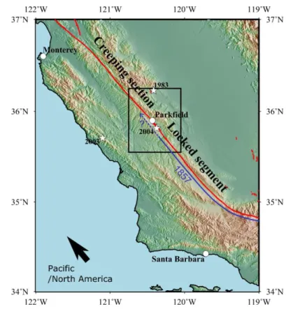
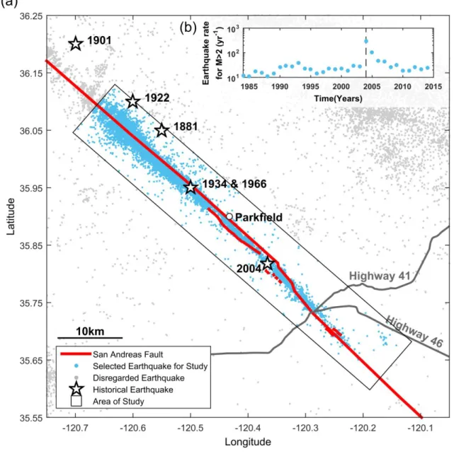
Here, we test and refine this approach on the Parkfield segment of the San Andreas fault. This
62
segment lies at the transition zone between the locked segment of the San Andreas Fault (SAF)
63
to the south and the creeping zone in the north (Figure 1). It has experienced six Mw ~ 6 64
earthquakes since the Mw ~ 7.7 Fort Tejon event of 1857 [Sieh, 1978; Bakun et al., 2005]. 65
Owing to its quasi-periodic behavior and occurrence of the latest Mw6.0 earthquake in 2004, 66
this section of the SAF has been intensively studied. These studies have yielded good
67
constraints on co- and postseismic deformation related to the 2004 earthquake [Langbein et al.,
68
2005, 2006; Johanson et al., 2006; Murray and Langbein, 2006; Barbot et al., 2009; Bruhat et
69
al., 2011; Wang et al., 2012, 2014], transient slow-slip events [Murray and Segall, 2005], and 70
interseismic loading [Murray et al., 2001; Murray and Langbein, 2006; Johnson, 2013; Wang
71
et al., 2014; Jolivet et al., 2015; Tong et al., 2015]. Several studies have noted that strain build-72
up in the interseismic period does not seem to be balanced by the strain released by M~6 events,
73
given their rate since 1857 [Segall and Harris, 1987; Murray and Segall, 2002; Murray and
74
Langbein, 2006; Toké and Arrowsmith, 2006]. This finding has implications for seismic hazard, 75
4
as it implies that M~6 events should be more frequent, on the long-term average, than has been
76
observed since 1857, or that occasional larger events should occur. The amount of data and the
77
frequent Mw ~ 6 events makes the Parkfield segment of the SAF a particularly appropriate test 78
case to assess the possibility of constraining seismic hazard based on a moment budget
79
approach.
80
Hereafter, we first describe the methodology used in this study. We then apply it to the
81
Parkfield segment of the SAF and test the sensitivity of our results to various assumptions about
82
the contribution of aftershocks and postseismic deformation. We conclude that Mw > 6 83
earthquakes are required to close the budget and assess the impact of this result on seismic
84 hazard. 85 86
Method
87We base our approach on the assumption that the rate of moment deficit accumulating in the
88
interseismic period is, on average over the long-term, equal to the rate of moment released by
89
seismic and transient aseismic slip. Our objective is to derive a probabilistic estimate of the
90
magnitude of the largest possible earthquake along a fault segment, together with an associated
91
recurrence time for such an earthquake. To do so, we calculate the moment released by
92
observed seismicity and afterslip, and divide by the duration of the catalogue to get the average
93
moment release rate. We compare this estimate with the moment deficit rate derived from
94
models of interseismic strain. If the moment deficit rate is larger than the observed moment
95
release rate, the observed maximum magnitude earthquake might not be the most extreme event
96
that can occur along the fault segment. We thus explore the space of magnitude and frequency
97
of maximum magnitude earthquakes to find which events can balance the moment budget and
98
be plausible considering the current statistical distribution of earthquakes. We account for
5
aftershocks, background seismicity and postseismic slip for each maximum magnitude
100
earthquake tested. This method allows to assess seismic hazard considering uncertainties on
101
the seismic and geodetic data and accounting for our understanding of the behavior of a fault
102
segment. In the following, we detail the method. A flow chart describing the approach, step by
103
step, is available in the supplementary (Table S.1). Table 1 lists the parameters used in this
104
study.
105
The rate of moment deficit accumulation, 𝑚̇0 (in N.m.yr-1), can be written
106
𝑚̇0 = ∫𝐹𝑎𝑢𝑙𝑡𝜇 𝐷 𝑑𝐴, (1)
where 𝜇 and 𝐴 are the shear modulus and the fault area, and 𝐷 is the slip deficit rate. The slip
107
deficit rate can be expressed as 𝐷 = 𝑉𝑝𝑙𝑎𝑡𝑒∗ 𝜒 where 𝑉𝑝𝑙𝑎𝑡𝑒 is the long-term plate rate and 𝜒 is
108
the interseismic coupling. The interseismic coupling is defined as the ratio between the deficit
109
of slip and the long-term slip of the fault and is given by
110
𝜒 = 1 −𝑉 𝑆 𝑝𝑙𝑎𝑡𝑒,
(2)
where 𝑆 is the creep rate observed during the interseismic period. 𝜒 is 0 for a fault patch
111
creeping at the long-term slip rate and 1 for a fully locked patch.
112
The amount of moment released seismically can be estimated from earthquake catalogues, for
113
example an historical catalogue. The average total seismic moment released per year 𝑚̇𝑆 is
114 given by 115 𝑚̇𝑆 = ∑𝑁𝑗=1𝑚𝑆,𝑗 𝑡ℎ𝑖𝑠𝑡 , (3)
where 𝑁 is the total number of events in the catalogue, 𝑚𝑆,𝑗 is the seismic moment of each
116
earthquake 𝑗 and 𝑡ℎ𝑖𝑠𝑡 is the time period covered by the catalogue. The observed seismicity
117
might be seen as one particular realization of a stochastic process over a certain period of time.
118
It might not be representative of the long-term average seismic moment rate if the period of
6
time covered by the data is short compared to the return period of the largest possible
120
earthquake.
121
The moment released by the known seismicity most often does not balance the moment deficit
122
due to interseismic coupling. Many causes can lead to a deficit of seismicity ( 𝑚̇0 > 𝑚̇𝑆): (1) 123
the largest possible earthquake is not present in the catalogue because of its too short time span;
124
(2) the largest possible earthquake is present in the catalogue but the duration of the catalogue
125
is longer than the average return period of such an event; (3) the undetected seismicity
126
contributes significantly to the moment budget; (4) transient aseismic slip such as afterslip or
127
slow slip events contribute significantly to the moment budget; (5) a fraction of interseismic
128
strain is anelastic and aseismic and is therefore not to be released seismically; (6) a large
129
earthquake with its epicenter outside the study area may have extended into the area of interest
130
and released a fraction of the moment deficit. In this case, the catalogue does not capture the
131
event. In the context of this study, this could have happened during the M~7.7 1857 Fort Tejon
132
mainshock or possibly as a foreshock. This earthquake ruptured the San Andreas Fault south
133
of Parkfield (Figure 1) and might have ruptured the Parkfield segment as well [Sieh, 1978].
134
Alternatively, 𝑚̇𝑆, the rate of moment released seismically, can exceed 𝑚̇0, the rate of moment 135
build up: (1) the largest possible event is in the catalogue but the period of time covered by the
136
catalogue is shorter than the average return period of such an event; (2) such events have
137
occurred more frequently over this period of time than over the long term average; (3)
138
interseismic strain is not stationary in time and the period covered by the geodetic data
139
corresponds to a loading rate that is less than the average over the long term. In any case, the
140
comparison between 𝑚̇𝑆 and 𝑚̇0 provides information on the magnitude and average return 141
period of the largest earthquake needed to balance the slip budget on the long term.
7
The next step consists in calculating the probability of a seismicity model to balance the
143
moment budget and be consistent with the known seismicity. Key parameters of the seismicity
144
model are the magnitude and return period of the largest earthquake.
145
The probability that the largest event is of magnitude 𝑀𝑚𝑎𝑥 and has on average a return period 146
of 𝜏𝑚𝑎𝑥 can be written as the product of two probabilities,
147
𝑃(𝑀𝑚𝑎𝑥, 𝜏𝑚𝑎𝑥) = 𝑃𝐵𝑢𝑑𝑔𝑒𝑡(𝑀𝑚𝑎𝑥, 𝜏𝑚𝑎𝑥) ∗ 𝑃𝐻𝑖𝑠𝑡(𝑀𝑚𝑎𝑥, 𝜏𝑚𝑎𝑥) . (4) 𝑃𝐵𝑢𝑑𝑔𝑒𝑡(𝑀𝑚𝑎𝑥, 𝜏𝑚𝑎𝑥) is the probability that an earthquake of magnitude 𝑀𝑚𝑎𝑥 and its 148
associated aftershocks and aseismic afterslip release a moment equal to the deficit of moment
149
accumulated over the return period 𝜏𝑚𝑎𝑥 (i.e. the probability that an earthquake of magnitude
150
𝑀𝑚𝑎𝑥 balances the budget). 𝑃𝐻𝑖𝑠𝑡(𝑀𝑚𝑎𝑥, 𝜏𝑚𝑎𝑥) is the probability that an event of 151
magnitude 𝑀𝑚𝑎𝑥 and return period 𝜏𝑚𝑎𝑥 is the maximum possible earthquake based on the 152
historical seismicity.
153
We calculate 𝑃𝐵𝑢𝑑𝑔𝑒𝑡 based on the assumption that the maximum-magnitude earthquake is
154
followed by aftershocks and that aseismic afterslip releases a moment proportional to the
155
moment released seismically. For a given mainshock moment magnitude and recurrence time,
156
we compare the moment released by the mainshock and postseismic relaxation (aftershocks
157
and aseismic afterslip) to the estimated rate of moment deficit building up on the fault.
158
Interseismic models of fault coupling derived using a Bayesian approach directly provide the
159
Probability Density Function (PDF) of the rate of moment accumulation [Wang et al., 2014;
160
Jolivet et al., 2015]. 161
We assume that, on average over the long-term, seismicity follows the empirical
Gutenberg-162
Richter (GR) law [Gutenberg and Richter, 1944]
163
8
where 𝑎 and 𝑏 are constants relating respectively to the total number of earthquakes recorded
164
per year and the relative distribution between small and large earthquakes, and 𝑁𝑀 is the 165
cumulative number of earthquakes per year over magnitude 𝑀. We assume that the law applies
166
to a catalogue of independent events (with aftershocks removed through ‘declustering’) as well
167
as to dependent events (a catalogue including aftershocks) and that the b-value is the same in
168
both cases (for a same given area). These assumptions are for examples consistent with the
169
earthquake statistics observed in Southern California [Marsan and Lengline, 2008].
170
The number of events per year with magnitudes in the range [ 𝑀 −𝜕𝑀2 , 𝑀 +𝜕𝑀2 ] , is then
171
𝑟 = 10𝑁𝑀−𝜕𝑀2 − 10𝑁𝑀+𝜕𝑀2
. (6)
The moment release rate of earthquakes with moment between 0 and 𝑚𝑎, over a period of time, 172
should then converge (in the limit of infinite time) towards
173
𝑚̇𝑆𝑎 = ∫ 𝑚𝑎 𝑟 𝑑𝑚
0 . (7)
We assume that earthquakes in the study area are bounded by a maximum event of moment
174
𝑚𝑚𝑎𝑥 and magnitude 𝑀𝑚𝑎𝑥. The largest aftershock has often a magnitude of about 1 unit less
175
than the magnitude of the mainshock [Båth, 1965] which might imply a bi-modal earthquake
176
distribution. Assuming that the background seismicity does not reach magnitudes larger than
177
the largest aftershock, the return period of the main event and that of the maximum aftershock
178
is the same and the GR relationship runs through 𝑀 = 𝑀𝑚𝑎𝑥 − 1 and 𝜏 = 𝜏𝑚𝑎𝑥.
179
However, the Båth law is not a physical law and is probably linked to a statistical finite size
180
effect (the number of aftershocks above a certain magnitude is finite and this finite number
181
determines the difference of magnitude between the mainshock and the largest aftershocks)
182
[Helmstetter and Sornette, 2003]. It is possible that at the limit of infinite time, although each
9
single cluster of earthquakes could follow the Båth law, the total GR distribution would apply
184
up to the maximum value of the distribution 𝑀 = 𝑀𝑚𝑎𝑥 and 𝜏 = 𝜏𝑚𝑎𝑥.
185
In the following, we test both cases and assume that these hypothesis bracket the contribution
186
to the total seismic moment release of earthquakes smaller than the maximum earthquake.
187
Additionally, we assume that the moment released by aseismic afterslip is a proportion 𝛼 of
188
the moment released seismically. Assuming that the moment release rate of seismic and
189
aseismic transient slip events balances the rate of moment deficit accumulation on the long run,
190
we get
191
𝑚̇0 = (𝑚̇𝑆𝑚+ 𝑚̇𝑆𝑎) (1 + 𝛼), (8)
where 𝑚̇𝑆𝑚 is the moment release rate of the largest earthquake (the subscript ‘S’ stands for
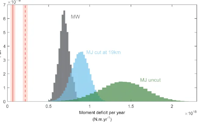
192
seismic and ‘m’ for mainshock), and 𝑚̇𝑆𝑎 the moment release rate of aftershocks and
193
background seismicity (the subscript ‘S’ stands for seismic and the subscript ‘a’ stands for
194
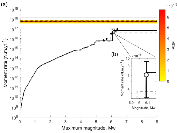
aftershock).
195
With the assumptions listed above, it is possible to calculate the probability 𝑃𝐵𝑢𝑑𝑔𝑒𝑡 of closing
196
the moment budget for a given magnitude and return period of the maximum earthquake.
197
Without taking the Båth law into account, this probability is highest along a straight line in the
198
Gutenberg-Richter plot corresponding to the return period of the largest event [Molnar, 1979;
199 Ader et al., 2012], 200 𝜏𝑚𝑎𝑥(𝑚𝑚𝑎𝑥) =1−2 𝑏/31 (1+𝛼) 𝑚𝑚̇ 𝑚𝑎𝑥 0 𝑖𝑓 𝑏 < 3/2, (9)
where 𝑚𝑚𝑎𝑥 is the moment released by the largest mainshock. With the Båth law, the
201
contribution of smaller events become nearly negligible,
202 𝜏𝑚𝑎𝑥(𝑚𝑚𝑎𝑥) = 10−3 𝐵2 1 − 2 𝑏/3 (1 + 𝛼) 𝑚𝑚𝑎𝑥 𝑚̇0 , (10)
10
with 𝐵 the difference in magnitude between the largest event and its largest aftershock. The
203
probability density distribution 𝑃𝐵𝑢𝑑𝑔𝑒𝑡 depends on the uncertainties on 𝑚̇0.
204
To illustrate the procedure, let us consider a magnitude of 7 with a return time of 𝜏𝑚𝑎𝑥. The
205
mainshock would release a moment of 3.5 1019 N.m. We add to this moment the contribution
206
of aftershocks, background seismicity and aseismic afterslip. The resulting moment is divided
207
by 𝜏𝑚𝑎𝑥 to estimate the average moment release rate for the events of magnitude 7 and return
208
period 𝜏𝑚𝑎𝑥. We compare this moment release rate to the rate of accumulation of moment
209
deficit in the interseismic period calculated from interseismic slip rate models.
210
Without any other constraint, the maximum possible magnitude on a fault that is accumulating
211
moment deficit at a rate 𝑚̇0 is actually unbounded: a small and frequent largest earthquake
212
would balance the moment budget as well as a larger infrequent one. Seismicity observations
213
can be used to tighten the space of possible solutions and incorporated through the calculation
214
of 𝑃𝐻𝑖𝑠𝑡(𝑀𝑚𝑎𝑥, 𝜏𝑚𝑎𝑥). This probability represents the probability of the largest earthquake
215
having a magnitude 𝑀𝑚𝑎𝑥 and a return period 𝜏𝑚𝑎𝑥 given the known seismicity. To calculate 216
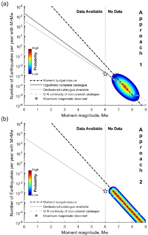
this probability, we consider two approaches:
217
Approach 1: We assume that the magnitude and frequency of the maximum-magnitude
218
earthquake falls on the GR law derived from a declustered catalog of local seismicity.
219
This hypothesis is questionable as it is not proven that the GR law applies up to the
220
largest possible event at a local scale;
221
Approach 2: The possible magnitude and frequency of the maximum-magnitude
222
earthquake must be consistent with the observed largest event over the observation
223
period (it has to be larger than or equal to the known largest event, and the return period
224
of the larger event cannot be significantly smaller than the observation period)
11
In both cases, a model of inter-event time distribution is required. In the results presented here,
226
we consider that independent events follow a Poisson process. This is probably a reasonable
227
assumption for events that would rupture only a fraction of the studied fault segment, as two
228
successive events would generally not occur at the same location, so that rebuilding stresses
229
might not be required. For larger events, it might be more appropriate to assume a
renewal-230
time model. In the supplement, we show the results obtained using a Brownian Passage Time
231
model [Matthews et al., 2002; Field and Jordan, 2015], which are only marginally different
232
from the ones obtained with the Poisson model.
233
In the case of a Poisson model, the probability of 𝑛 events occurring during the time period 𝑡
234
is
235
𝑃𝑝𝑜𝑖𝑠𝑠𝑜𝑛(𝑛, 𝑡, 𝜏) =(𝑡/𝜏)𝑛!𝑛𝑒−𝑡/𝜏, (11)
where 𝜏 is the average recurrence time of the Poisson process.
236
Following the first approach, the probability of (𝑀𝑚𝑎𝑥, 𝜏𝑚𝑎𝑥) being the magnitude and return
237
period of the largest event depends on the magnitude of the largest observed earthquake 𝑀ℎ𝑖𝑠𝑡 238
and on the return period 𝜏𝐺𝑅(𝑀𝑚𝑎𝑥) predicted by the GR law derived from a declustered
239 catalog: 240 𝑖𝑓 𝑀𝑚𝑎𝑥 < 𝑀ℎ𝑖𝑠𝑡, 𝑃𝐻𝑖𝑠𝑡(𝑀𝑚𝑎𝑥, 𝜏𝑚𝑎𝑥) = 0, (12) 𝑖𝑓 𝑀𝑚𝑎𝑥 > 𝑀ℎ𝑖𝑠𝑡, 𝑃𝐻𝑖𝑠𝑡(𝑀𝑚𝑎𝑥, 𝜏𝑚𝑎𝑥) ∝ 𝑃𝑝𝑜𝑖𝑠𝑠𝑜𝑛(𝑛 = 1, 𝜏𝑚𝑎𝑥, 𝜏𝐺𝑅(𝑀𝑚𝑎𝑥)) = (𝜏𝑚𝑎𝑥/𝜏𝐺𝑅(𝑀𝑚𝑎𝑥))𝑒−𝜏𝑚𝑎𝑥/𝜏𝐺𝑅(𝑀𝑚𝑎𝑥). (13)
We use the sign ∝ to indicate proportionality, as the PDF is normalized.
241
Following the second approach, the probability of (𝑀𝑚𝑎𝑥, 𝜏𝑚𝑎𝑥) being the magnitude and 242
return period of the largest event depends on the magnitude of the largest observed earthquake
12
𝑀ℎ𝑖𝑠𝑡 and on time period covered by the catalog 𝑡ℎ𝑖𝑠𝑡. It can be defined as the probability to 244
have no earthquakes of magnitude over 𝑀ℎ𝑖𝑠𝑡 occurring during the time period of the catalog: 245 𝑖𝑓 𝑀𝑚𝑎𝑥 < 𝑀ℎ𝑖𝑠𝑡, 𝑃𝐻𝑖𝑠𝑡(𝑀𝑚𝑎𝑥, 𝜏𝑚𝑎𝑥) = 0, (14) 246 𝑖𝑓 𝑀𝑚𝑎𝑥 > 𝑀ℎ𝑖𝑠𝑡, 𝑃𝐻𝑖𝑠𝑡(𝑀𝑚𝑎𝑥, 𝜏𝑚𝑎𝑥) ∝ 𝑃𝑝𝑜𝑖𝑠𝑠𝑜𝑛(𝑛 = 0, 𝜏ℎ𝑖𝑠𝑡, 𝜏𝑚𝑎𝑥) = 𝑒− 𝑡ℎ𝑖𝑠𝑡 𝜏𝑚𝑎𝑥. (15)
The probability drops rapidly to zero as 𝜏𝑚𝑎𝑥 becomes smaller than 𝑡ℎ𝑖𝑠𝑡. It becomes uniform 247
quickly as 𝜏𝑚𝑎𝑥 gets larger than 𝑡ℎ𝑖𝑠𝑡.
248
Figure 2 shows a schematic representation of the probability 𝑃𝐵𝑢𝑑𝑔𝑒𝑡∗ 𝑃𝐻𝑖𝑠𝑡 in both cases. In
249
the first case, the probability that an earthquake is the maximum possible earthquake in view
250
of the observed seismicity and also closes the moment budget is highest at the intersection
251
between the GR law (equation 4) and the line representing the return period of the largest
252
earthquake required to close the moment budget (equation 9 or 10). In the second case, the
253
probability that an earthquake is the maximum possible earthquake in view of the observed
254
seismicity and also closes the moment budget is highest along the line representing the budget
255
closure condition (equation 9 or 10). Any large magnitude (𝑀𝑚𝑎𝑥 > 𝑀ℎ𝑖𝑠𝑡) and very infrequent 256
maximum earthquake that closes the moment budget is considered acceptable as long as its
257
return period is long compared to the observation period (𝜏𝑚𝑎𝑥 > 𝑡ℎ𝑖𝑠𝑡). 258
In principle, we could also use phenomenological scaling laws, or physical constraints [Scholz,
259
1982] to limit the range of possible earthquake magnitude on a particular fault segment. For
260
instance, we could impose the co-seismic stress drop to be between 0.1MPa and 100MPa, as
261
generally observed [e.g., Kanamori and Brodsky, 2004]. This would constrain the maximum
262
possible moment given the size of the locked area. We find such constraints to be too loose to
13
be useful and are therefore not included as an a priori in our analysis. We use them a posteriori
264
to validate our assessment qualitatively.
265
When it comes to seismic hazard, the two methods should not yield much different outcomes
266
if the hazard is calculated over a period of time 𝑡 similar in duration to the earthquake catalog
267
𝑡ℎ𝑖𝑠𝑡. They could however differ significantly for 𝑡 ≫ 𝑡ℎ𝑖𝑠𝑡. To assess the impact of choosing
268
between approaches 1 and 2, we calculate the probability 𝑃𝐻𝑎𝑧𝑎𝑟𝑑(𝑀 > 𝑀𝑇𝑒𝑠𝑡, 𝑡) of an
269
independent event over a period 𝑡 exceeding a magnitude 𝑀𝑇𝑒𝑠𝑡 for different values of 𝑡. The
270
probability 𝑃𝐻𝑎𝑧𝑎𝑟𝑑 of an independent event with magnitude > 𝑀𝑇𝑒𝑠𝑡 during a period of time 271 𝑡 is 272 𝑃𝐻𝑎𝑧𝑎𝑟𝑑(𝑀 > 𝑀𝑇𝑒𝑠𝑡, 𝑡, 𝜏𝑀) = 1 − 𝑃𝑝𝑜𝑖𝑠𝑠𝑜𝑛(𝑛 = 0, 𝑡, 𝜏𝑀) = 1 − 𝑒− 𝑡 𝜏𝑀, (16) where 𝜏𝑀 is the average recurrence time of independent earthquakes with magnitude larger
273
than 𝑀𝑇𝑒𝑠𝑡which can be calculated from the Gutenberg-Richter law (𝜏𝑀 = 10−(𝑎−𝑏 𝑀𝑇𝑒𝑠𝑡), with 274
a and b being determined from a ‘declustered’ catalog). The probability 𝑃𝐻𝑎𝑧𝑎𝑟𝑑 calculated this
275
way does not account for aftershocks.
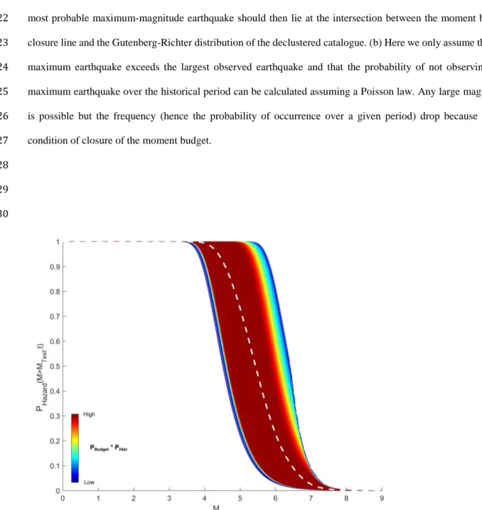
276
To construct Figure 3 we first choose a value of t. We then grid the magnitude-frequency space
277
and test systematically all magnitudes of the maximum possible earthquake and all the return
278
periods within a search area. For each sample tested, we represent the probability
279
𝑃𝐻𝑎𝑧𝑎𝑟𝑑(𝑀 > 𝑀𝑇𝑒𝑠𝑡, 𝑡) with a curve shaded according to the probability 𝑃𝐵𝑢𝑑𝑔𝑒𝑡∗ 𝑃𝐻𝑖𝑠𝑡. We
280
can thus apprehend visually the most likely earthquake scenarios that might happen during the
281
time period 𝑡 (Figure 3). A mean probability of all the possibilities tested, which we weight
282
with the product 𝑃𝐵𝑢𝑑𝑔𝑒𝑡∗ 𝑃𝐻𝑖𝑠𝑡, can be obtained from equation
283
𝑃̅𝐻𝑎𝑧𝑎𝑟𝑑(𝑀 > 𝑀𝑇𝑒𝑠𝑡, 𝑡) =
∑𝑁𝑘=1𝑃𝐻𝑎𝑧𝑎𝑟𝑑,𝑘∗𝑃𝐵𝑢𝑑𝑔𝑒𝑡,𝑘∗𝑃𝐻𝑖𝑠𝑡,𝑘
∑𝑁𝑘=1𝑃𝐵𝑢𝑑𝑔𝑒𝑡,𝑘∗𝑃𝐻𝑖𝑠𝑡,𝑘 ,
14
where 𝑁 is the number of samples tested, 𝑘 is the sample index, 𝑃𝐻𝑎𝑧𝑎𝑟𝑑,𝑘 is the probability of
284
an independent event with magnitude >𝑀𝑇𝑒𝑠𝑡 during the time period 𝑡 for the sample 𝑘, and
285
𝑃𝐵𝑢𝑑𝑔𝑒𝑡,𝑘∗ 𝑃𝐻𝑖𝑠𝑡,𝑘 is the probability of sample 𝑘 given the seismicity observations and the 286
moment budget closure condition.
287
To illustrate the procedure, let us first choose a sample of maximum magnitude, 𝑀𝑚𝑎𝑥, and its
288
time recurrence, 𝜏𝑚𝑎𝑥. We assume that this event belongs to a distribution of independent
289
events that follows the GR law. Choosing 𝑀𝑇𝑒𝑠𝑡= 4 (for example), we can calculate the
290
probability of having an independent earthquake over magnitude 4 during a time period 𝑡,
291
knowing that those events have a recurrence time given by the GR law (equation 16). Applying
292
this to the full range of 𝑀𝑇𝑒𝑠𝑡 ∈ [0, 𝑀𝑚𝑎𝑥], 𝑃𝐻𝑎𝑧𝑎𝑟𝑑 will be represented by a line in Figure 3. 293
This 𝑃𝐻𝑎𝑧𝑎𝑟𝑑 is associated with a specific 𝑀𝑚𝑎𝑥 and 𝜏𝑚𝑎𝑥, and corresponds to a specific
294
𝑃𝐵𝑢𝑑𝑔𝑒𝑡(𝑀𝑚𝑎𝑥, 𝜏𝑚𝑎𝑥) ∗ 𝑃𝐻𝑖𝑠𝑡(𝑀𝑚𝑎𝑥, 𝜏𝑚𝑎𝑥). If we test each possible 𝑀𝑚𝑎𝑥 and 𝜏𝑚𝑎𝑥, and plot
295
their 𝑃𝐻𝑎𝑧𝑎𝑟𝑑 in the same representation, the shade of each line indicating 𝑃𝐵𝑢𝑑𝑔𝑒𝑡∗ 𝑃𝐻𝑖𝑠𝑡, we
296
then obtain Figure 3. We could then calculate the average 𝑃𝐻𝑎𝑧𝑎𝑟𝑑 of all those lines, but it 297
would not account for the probability to close the moment budget and be plausible considering
298
the observed seismicity. We then weight each 𝑃𝐻𝑎𝑧𝑎𝑟𝑑 obtained for a particular choice of 𝑀𝑚𝑎𝑥
299
and 𝜏𝑚𝑎𝑥 by its related 𝑃𝐵𝑢𝑑𝑔𝑒𝑡∗ 𝑃𝐻𝑖𝑠𝑡, and use this to calculate the weighted average 𝑃̅𝐻𝑎𝑧𝑎𝑟𝑑
300
(equation 17) represented by the white dashed line in Figure 3.
301
We sample the probabilities using the Hasting-Metropolis Monte Carlo Markov Chain
302
(MCMC) procedure [Metropolis et al., 1953; Hasting, 1970]. We calculate for each sample 𝑘,
303
with a given magnitude and frequency of the largest earthquake, the probability that it is
304
realistic knowing the data 𝑃𝐻𝑖𝑠𝑡,𝑘 and the probability that it closes the budget 𝑃𝐵𝑢𝑑𝑔𝑒𝑡,𝑘. The
305
final probability 𝑃𝐺,𝑘 (i.e. the posteriori probability) of a given sample would thus be
15
𝑃𝐺,𝑘 ∝ 𝑈𝑀𝑈𝐹𝑟𝑒𝑞𝑃𝐵𝑢𝑑𝑔𝑒𝑡,𝑘𝑃𝐻𝑖𝑠𝑡,𝑘, (18)
where 𝑈𝑀 and 𝑈𝐹𝑟𝑒𝑞 are the uniform laws chosen for the MCMC sampling for the magnitude
307
and frequency, respectively (i.e. the a priori probability).
308 309
Application to the Parkfield segment of the San Andreas Fault
310
Moment budget
311
Interseismic strain around the Parkfield segment of the San Andreas fault has been investigated
312
in a number of recent studies [Johnson, 2013; Wang et al., 2014; Jolivet et al., 2015; Tong et
313
al., 2015]. Here we rely on the studies of Wang et al. [2014] and Jolivet et al. [2015], as they 314
provide a probabilistic description of slip rate from Bayesian inversions which can be directly
315
used as an input in our study. We consider the same fault geometry and focus on the same fault
316
area as Wang et al. [2014] (Figure 4 and 5). To assess the moment budget, we use interseismic
317
models from Wang et al. [2014] and Jolivet et al. [2015] which were both derived from
318
inversion of interseismic displacements measured at the surface assuming a fault embedded in
319
an elastic medium. Wang et al. [2014] assumed a homogeneous elastic half-space and Jolivet
320
et al. [2015] considered depth variations of elastic moduli. We convert slip potency (the 321
integral of slip over fault area) to moment according to the elastic structure assumed in these
322
studies.
323
Wang et al. [2014] present three different Bayesian inversions of GPS data from 14 stations
324
covering the period from 1999 to 2004 including the mainshock of 2004 and 5 days of
325
postseismic relaxation. They use a 70km long, ~19 km deep fault subdivided into 180 patches,
326
each 1.4 km long along strike and 1 km wide. A steady slip rate is assumed at depth greater
327
than 19 km. We considered their favored model (referred to as MW hereafter), which was
328
obtained from a joint inversion of the interseismic, co-seismic and 5-days postseismic data,
16
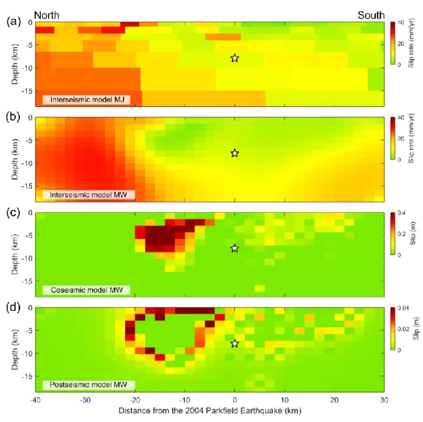
designed to maximize the consistency between the three slip distributions. The slip
330
distributions are therefore complementing each other (Figure 4): the co-seismic rupture is
331
restricted to the area that was locked during the interseismic period; the inversions assume that
332
postseismic slip is driven by the co-seismic stress change and thus yields a ring of afterslip
333
surrounding the co-seismic rupture. The steady slip rate on the deeper extension of the fault is
334
estimated to 32.1 mm/yr in this model. The Bayesian framework provides uncertainties on all
335
quantities determined from the inversion.
336
Jolivet et al. [2015] (MJ) also used a Bayesian approach and derived an interseismic model
337
from GPS and InSAR data covering the period from 2006 to 2010. The modeled fault zone
338
extends over 200 km from the Cholame plain to north of San Juan Baptista (SJB). The patch
339
size varies depending on the resolution from 4 km at the surface to 25 km at 20 km depth. The
340
long-term slip rate varies along strike. In the Parkfield area considered in this study, it varies
341
from 31.1 mm/yr to 36.6 mm/yr. The model shows a gradual northward decrease of
342
interseismic coupling from the locked zone in the southeast to the creeping zone in the
343
northwest (Figure 4). This model shows a deficit of slip extending to depth greater than 19km,
344
thus deeper than the seismogenic depth. Given the absence of seismicity at such depth and the
345
fact that temporal variations of strain rates in this depth range are probably primarily due to
346
viscoelastic relaxation as was observed following the 2004 earthquake [Bruhat et al., 2011],
347
we consider slip deficit accumulation only in the 0-19km depth range of our fault model.
348
Both models yield deep slip rates in agreement with the geological long term slip rate on the
349
SAF which is estimated to 33.9±2.9mm/yr in the Carrizo plain south of the Parkfield segment
350
[Sieh and Jahns, 1984]. These rates are also consistent with those (34.9-36.0±0.5mm/yr)
351
derived from elastic block modeling of regional tectonics [Meade and Hager, 2005; Tong et
352
al., 2014]. They are, however, larger than the local estimate of 26.2 +6.4/- 4.3mm/yr of Toké 353
et al. [Toké et al., 2011]. Both models show high interseismic coupling in the area that ruptured
17
in 2004. They differ significantly in part because they use different interseismic observations
355
but also because of different methods and a priori assumptions. In addition to enforcing
356
consistency between the three phases of the earthquake cycle, the inversion used to derive MW
357
was regularized via spatial smoothing. By contrast MJ was obtained without any constraint on
358
the smoothness of the slip rate distribution nor on the relationship between interseismic and
359
co-seismic slip. Note that the long-term slip-rate on the continuation of the fault at the depth is
360
constant in MW but varies along strike in MJ. For MJ, fault patches are assigned the long-term
361
slip rate of the deeper creeping patches. Those located astride different deep creeping patches
362
are divided in sub-patches. The shear modulus used to convert slip to moment is 30GPa for
363
MW and varies between 20.5GPa and 66.2GPa for MJ [Jolivet et al., 2015].
364
The Bayesian approach used in Jolivet et al. [2015] and Wang et al. [2014] provides thousands
365
of scenarios, which were tested against geodetic data. For both studies, we calculate the
366
moment deficit rate of every scenario using equation 1 and 2 to derive the PDF of the moment
367
deficit rate. The rate of accumulation of moment deficit for each model is indicated in Table 2
368
and the corresponding PDFs are shown in Figure 6.
369
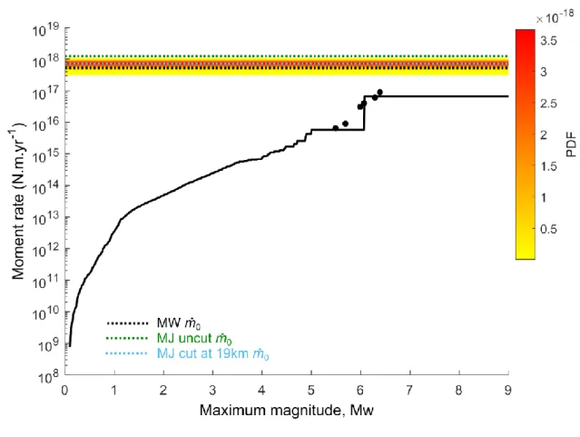
We calculated and represented in Figure 7 the moment deficit rate on a completely locked 70
370
x 20 km section loaded at 32.1 mm/yr (full black line) and a section with the coupling pattern
371
from the MW model (black dashed line). Based on interseismic model MW the moment deficit
372
builds up at a rate of 6.90 +/- 0.64 1017 N.m/yr. The PDF associated with this estimate is shown
373
in Figure 6. Some of this deficit was released by aseismic afterslip following the 2004 event
374
which released about 3.7 1018 N.m Bruhat et al. [2011]. We do not use the afterslip model of
375
Wang et al. [2014], as their model covers only 5 days after the mainshock. The dotted line in
376
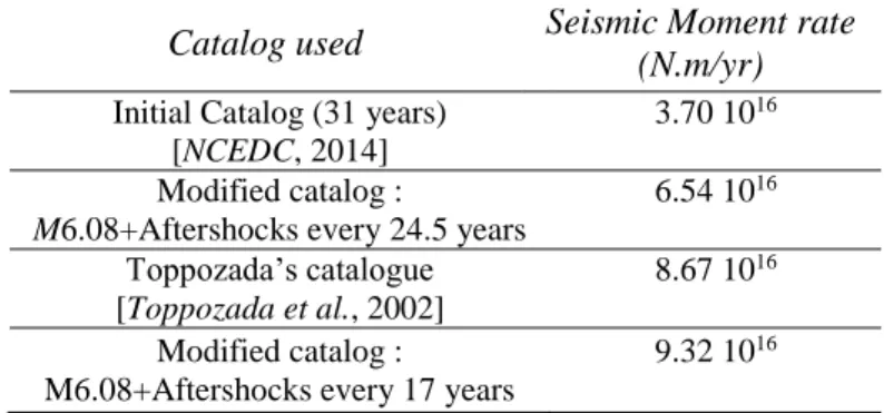
Figure 7 shows the remaining deficit of moment which amounts to 5.39 1017 N.m/yr.
18
Based on interseismic model MJ, the moment deficit accumulates in the interseismic period at
378
a rate as large as 8.82 +/- 1.10 1017 N.m/yr (Figures 6). The difference with the rate obtained 379
with MW is partly due to the different pattern of coupling and to the difference of deep creep
380
rates (31.1 and 36.5 mm/yr for MJ and 32.1 mm/yr for MW). The rate is reduced to 7.31 1017
381
N.m/yr if aseismic afterslip is substracted (Figure 8).
382
The moment released by seismicity is estimated from the Northern California earthquake
383
catalog [NCEDC, 2014] from 1984 to 2015 (up to 5/2/2015). We consider earthquakes located
384
within 5 km of the fault (Figure 5). Figure 7 shows the cumulative moment released by
385
earthquakes of magnitude under 𝑀 taken directly from the catalog (gray dashed line). This
386
estimate might not be representative of the interseismic cycle. The inset in Figure 5 shows
387
minor temporal fluctuations except for the strong increase of seismicity associated to the 2004
388
aftershocks. The moment released by seismicity over the 31 years covered by the catalog,
389
representative of the 2004 event (87%), its aftershocks (7%) and the background seismicity
390
(6%), accounts for only 5% of the deficit of moment that has accumulated over this time period
391
according to the interseismic model MW, or 7% if the postseismic moment released is taken
392
into account (Figure 7). It represents an even lower fraction (4%) of the deficit of moment
393
calculated based on the interseismic model MJ (5% if taking into account the aseismic moment
394
released by afterslip; Figure 8). As mentioned above, the deficit could suggest that the return
395
period of the maximum magnitude earthquake is over-estimated or that larger magnitude events
396
are needed on this fault segment. We now consider the first possibility.
397
Six 𝑀𝑤~6 earthquakes occurred at Parkfield between 1857 and 2004, yielding an average
398
return period of 24.5 years. The catalog covers 31 years and includes the 2004 event and its
399
aftershocks. Some corrections might thus be needed to represent the long-term average
400
seismicity. Let us assume that the 2004 Parkfield earthquake is characteristic of the sequence
401
of 𝑀𝑤 6 earthquakes that have occurred since 1857. We assume that such an event and its
19
associated aftershocks, return every 24.5 ± 9.2 year on average, where the uncertainty is the
1-403
sigma standard deviation of the time intervals. We consider the moment released by such an
404
event to be equal to the mean moment estimated for 2004 from various publications [Johanson
405
et al., 2006; Langbein et al., 2006; Liu et al., 2006; Murray and Langbein, 2006; Barbot et al., 406
2009; Bruhat et al., 2011; NCEDC, 2014; Wang et al., 2014]. We use the standard deviation
407
of these estimates as an estimate of the uncertainty at the 67% confidence level. The average
408
moment released is then 1.48 1018 ± 4.7 1017N.m (𝑀𝑤 6.08).
409
We estimate the moment released by aftershocks by comparing the seismicity rate over the
410
2004-2008 period with the 1984-2004 period. We also assume that each event triggered as
411
much aseismic afterslip as the 2004 event. According to Bruhat et al., 2011, afterslip following
412
the 2004 event released about 1.57 1018 N.m assuming viscous flow under 19km depth, or about
413
3.7 1018 N.m if viscous relaxation is excluded, which is more than twice the coseismic moment
414
release. Hereafter we assume that afterslip released up to 200% of coseismic moment, which
415
gives us an upper-bound on the total moment released by this sequence of earthquake. The
416
moment released by afterslip is subtracted from the deficit of moment accumulating in the
417
interseismic period (Figure 7 and 8). The values corresponding to this moment budget estimate
418
are reported in Table 2 and Table 3, and illustrated in Figure 6, 7 and 8. Clearly, the moment
419
released by 2004-like events returning every 24.5 ± 9.2 year on average falls still way short of
420
balancing the moment budget (12.1% of MW’s model).
421
Returning 𝑀𝑤~6 earthquakes at Parkfield do not necessarily release the same moment as the
422
2004 event. The 1966 Parkfield earthquake is considered to be relatively similar to the 2004
423
one in terms of its moment release and rupture area [Bakun et al., 2005]. According to the
424
reported damages [Toppozada et al., 2002], the events of 1901 and 1922 may have been
425
stronger (𝑀𝑤 6.4 and 𝑀𝑤 6.3 respectively). Moreover, several 𝑀𝑤>5 earthquakes that
426
occurred between 1857 and 2015 are considered to be independent from the 𝑀𝑤~6 earthquake
20
(𝑀5.5 in 1877 and 𝑀5.8 in 1908), or direct aftershocks of the 1901 and 1922 earthquakes.
428
Figures 7 and 8 show that if we now consider the historical catalog of Toppozada et al. [2002],
429
the moment released by seismicity is higher but still too small to balance the moment budget
430
(Table 3). Assuming that the interseismic period covered by geodetic data is representative of
431
the long-term average, we derive that seismicity and afterslip released at most 16.1% (MW) of
432
the deficit of moment accumulated since 1857. The epicenter of the 1901 𝑀6.4 earthquake is
433
actually located slightly north of our study area. The damage distribution indicates that the
434
rupture propagated within the Parkfield area, but it is not sure that the rupture area was confined
435
to the fault area consider in our study. By assuming that the moment of this earthquake was
436
entirely released by slip on the fault segment considered in this study we probably tend to
437
overestimate the seismic moment release.
438
Considering this time only for the moment deficit rate from the seismogenic zone (~15km
439
depth) and reducing the recurrence time of the 𝑀6 to 17 years as estimated by [Wang et al.,
440
2015] does not close the moment budget either. The moment deficit rate is reduced to
3.86+/-441
0.52 1017 N.m/yr based on the interseismic model MW cut at 15km depth with afterslip
442
subtracted, and the seismic moment released is increased to 9.32 1016 N.m/yr. Giving this 443
extreme scenario, the percentage of seismic moment released compared to the moment deficit
444
rate is still low (24%).
445
Some coseismic models of the 2004 𝑀6 earthquake indicate slip up to 30km south of the
446
hypocenter [Wang et al., 2014, 2015] and a similar rupture extent to that proposed for the 1966
447
earthquake [Murray and Langbein, 2006]. However, most models indicate that the 2004
448
rupture did not go further than 10 km south of the hypocenter [Johanson et al., 2006; Liu et al.,
449
2006; Allmann and Shearer, 2007; Barbot et al., 2009; Bruhat et al., 2011]. By limiting the
450
extent of our area of study to 10 km south of the 2004 hypocenter and by cutting the
451
interseismic models at an even more shallower seismogenic zone (10km depth), we obtain a
21
moment deficit rate of 2.93 1017 N.m/yr for MW and 2.99 1017 N.m/yr for MJ. The moment
453
deficit rate PDF of the model MJ would then slightly overlap with the moment released by
454
earthquakes and postseismic slip. The probability to close the moment budget is nevertheless
455
2%. On the other hand, the MW model would still not overlap.
456
This analysis shows that balancing the moment budget on the Parkfield segment of the San
457
Andreas fault probably requires more frequent or larger earthquakes than what the instrumental
458
and historical data suggest. All the seismic moment release rate discussed in this section are
459
available in Table 3.
460
Note that Tong et al. [2015] integral method yields a moment deficit rate around 5.8 1017
461
N.m/yr, which is slightly smaller than the best fitting value of MW but within the uncertainty
462
range. We consider that the range of rates of moment deficit explored by using the Bayesian
463
inversions of MJ and MW models of interseismic coupling provides a reasonable estimate of
464
the range of possible values given the uncertainties on the geodetic data and choice of the
465
modeling technique.
466 467
Maximum-Magnitude Earthquake Evaluation
468
We now explore the range of possible magnitudes and frequencies for the largest possible
469
earthquake needed to balance the moment budget. We first compute the probability of closing
470
the moment budget for a given magnitude and frequency for the largest possible earthquake.
471
We next calculate the probability of the possible earthquake models based on either approach
472
1 (seismicity follows the Gutenberg-Richter law up to the largest possible earthquake) or 2
473
(larger earthquakes can fall off the Gutenberg-Richter distribution indicated by instrumental
474
and historical data).
22
We use the MCMC method to sample these probabilities. Each sample is taken from a uniform
476
PDF between 6.4 and 9 for magnitudes, and between 10-6 and 104 yrs-1 for frequencies. We 477
calculate for each sample 𝑘 the value proportional to the probability 𝑃𝐺,𝑘 as described in the 478
method section. For each estimation, we run the sampler for 900000 steps, rejecting the first
479
500 steps to ensure accurate sampling of the PDF. The magnitude-frequency space is then
480
binned into cells of size 0.01 for the moment magnitude axis and logarithmically binned into
481
cells of size 0.01 concerning the frequency axis. The number of samples in each cell divided
482
by the total number of samples approximates the probability 𝑃𝐺,𝑘 as defined by the MCMC
483
method.
484 485
Moment Budget closure, 𝑷𝑩𝒖𝒅𝒈𝒆𝒕
486
We calculate the probability 𝑃𝐵𝑢𝑑𝑔𝑒𝑡,𝑘 of closing the moment budget based on the uncertainties
487
on the parameters of interseismic models MJ or MW. We estimate the moment released by
488
seismicity for a tested magnitude Mk and recurrence time 𝜏k of the largest earthquake and 489
estimate the probability that it balances the moment budget using interseismic models MJ or
490
MW. The probabilities on the interseismic models are taken from the distribution of their
491
moment deficit using a bin of 1016 N.m.
492
The moment released by aftershocks and independent events with magnitude smaller than the
493
largest earthquake is integrated by assuming that their magnitude-frequency distribution
494
follows the GR law. We consider two cases. In the first case, the aftershocks and independent
495
events follow the GR law up to the largest earthquake included. In the second case, we account
496
for Båth law; the largest aftershock is 1 unit of magnitude unit lower than the mainshock, as it
497
is observed in the 2004 event. We suppose also that the b-value is constant and equal to the one
498
estimated from the modified 1984-2015 catalog. We use the maximum curvature method
23
[Wiemer and Wyss, 2000] and Bender’s formula [Aki, 1965; Utsu, 1966; Bender, 1983] to
500
evaluate the magnitude of completeness and the b-value. The estimated magnitude of
501
completeness is increased by 0.2 to compensate a methodological bias of the method [Woessner
502
and Wiemer, 2005]. The b-value, estimated at 0.91±0.06, is then used to account for the 503
magnitude-frequency distribution of both aftershocks and independent events. The a-value is
504
easily calculated from equation (5).
505
Moment released by aseismic afterslip is accounted for by supposing that, for all earthquakes,
506
it amounts to a fixed percentage of the seismic moment. This percentage might in fact depend
507
on earthquake magnitude but the available data are insufficient to derive a reliable law [Lin et
508
al., 2013]. We considered a value of 25%, close to the mean value observed from various case 509
studies [Avouac, 2015], and a more extreme value of 200%, similar to that estimated for the
510
2004 earthquake. The value of 200% is an overestimation of Bruhat et al., [2011].
511 512
𝑷𝑯𝒊𝒔𝒕: First Approach
513
In the Method section, we proposed two different approaches regarding how the
frequency-514
magnitude of the largest possible earthquake might be evaluated based on the known
515
seismicity. The first case, the most restrictive, assumes that the distribution of a declustered
516
catalog follows the GR law up to the largest event. Some declustered catalogs are available for
517
California [Dutilleul et al., 2015] but they contain less than 200 earthquakes within 5 km from
518
the fault segment considered in our study. This small number does not permit any reliable
b-519
value estimation [Woessner and Wiemer, 2005]. Therefore, we will rely on a non-declustered
520
catalog.
521
Assuming a postseismic moment release equivalent to 200% of the mainshock seismic
522
moment, not accounting for Båth’s law and selecting MW as the interseismic model represents
24
the most “optimistic” situation where the magnitude of the largest earthquake needed to close
524
the moment budget is minimum. In this scenario, 𝑃𝐺 (Equation 18) peaks around ~𝑀7.6,
525
corresponding to a seismic moment of 2.8 1020 N.m, with a recurrence time period of ~3300 526
years (Figure 9). The release of such a large moment on a 70km long segment seems however
527
improbable, however, especially in view of the limited locked zone in the interseismic period.
528
The average slip in such an event, supposing that the whole fault ruptures (20x70 km) and
529
taking a 30GPa shear modulus, would be of ~7m. If we assume a rupture restricted to the
530
locked portion of this fault segment, which represents only 1/3 of the fault area, the average
531
slip would need to be as great as 21m. This seems highly improbable.
532
We note in Figure 9 that the magnitude-frequency distribution of instrumental earthquakes does
533
not align well with the historical seismicity. The earthquake rate is lower than expected if we
534
assume the GR law extends up to larger magnitudes. The misalignment could be due to various
535
causes. One is that the historical catalog essentially consists of independent events while the
536
instrumental catalog contains aftershocks. The two catalogs could belong to the same
537
Gutenberg-Richter distribution if the b-value of the declustered catalogs was lower than when
538
the aftershocks are included as some studies suggest [Frohlich and Davis, 1993]. Extrapolating
539
the Gutenberg-Richter law to the largest possible magnitude might be incorrect as a number of
540
studies have argued that larger magnitude events are more frequent than would be expected
541
from extrapolating the b-value estimated from lower magnitude seismicity [Schwartz and
542
Coppersmith, 1984]. Another possibility is that the seismicity rate between 1984 and 2015 543
would have been particularly low compared to a longer term average [Page and Felzer, 2015].
544
In both case, the method used here to estimate PHist would overestimate the magnitude of the 545
largest magnitude earthquake.
546
With the first approach, using the marginal cumulative probabilities, we can assess the
547
probability that the largest event does not exceed a certain magnitude and the frequency of the
25
largest event is inferior to a certain value (Figure 10.a and c). The probability of closing the
549
moment budget on the Parkfield segment of the San Andreas Fault with the magnitude of the
550
maximum earthquake not exceeding 6.4 is only 0.3%. Therefore, provided that the GR law is
551
valid up to magnitude M6.4, which seems a reasonable assumption, the analysis requires larger
552
earthquakes. Figure 10 indicates that there is a 95% chance that the maximum event does not
553
exceed a 𝑀8.63. There is also a 95% chance that the return period of the largest magnitude
554
event does not exceed ~112000 years. It seems very improbable that the Parkfield segment
555
could host an earthquake of such a magnitude as it would require 253m of slip in a 19x70km
556
area. The probability of balancing the moment budget with a maximum earthquake not
557
exceeding 7.4 is about 50%, indicating that even with such a large maximum earthquake,
558
balancing the moment budget remains unlikely if the GR law applies. Note that if the largest
559
earthquakes involve ruptures that extend beyond the Parkfield segment, our analysis only
560
provides constraints on the moment released within the Parkfield segment. In that case, the
561
assumption that this earthquake belongs to a GR distribution defined by earthquakes on the
562
Parkfield segment is certainly incorrect and the second approach is then more relevant.
563 564
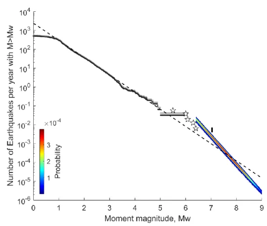
𝑷𝑯𝒊𝒔𝒕: Second approach
565
Our second approach only assumes that the largest possible earthquake needs to be less
566
frequent than the largest known earthquake. The probability of its return period is estimated
567
based on the historical catalog (only the duration of the period covered matters) assuming a
568
Poisson process. If we consider the interseismic model MW, discard the Båth law and assume
569
that postseismic deformation releases 200% of the coseismic moment we get a more reasonable
570
result than with approach 1 (Figure 11). A 𝑀6.7 every 140 years is then sufficient to balance
571
the moment budget and is acceptable in view of the known seismicity. This point aligns well
572
with the frequency-magnitude distribution of historical events but is off the distribution of
26
instrumental events, essentially because of the break in slope around M~4. This is our favored
574
scenario. Note, however, that the method does not exclude 𝑀 > 6.7 events.
575
Figure 12 shows that the PDF of the magnitude-frequency of the largest event varies depending
576
on the choice of the interseismic model (MJ or MW), on whether or not Båth’s law is accounted
577
for, and on the assumption that either 25% or 200% of the mainshocks seismic moment is
578
released by postseismic effects. The Båth law has a significant impact. If it is taken into
579
account, aftershocks and independent events amount to only ~8% of the moment released by
580
the largest earthquake compared to ~156% if the Båth law is discarded. Consequently, when
581
the Båth law is not accounted for, the aftershocks and independent events sequence decrease
582
drastically the maximum-magnitude needed for budget closure. Similarly, postseismic
583
deformation amplifies the moment released by the largest earthquake, its aftershocks and the
584
associated independent events. The higher the ratio between the postseismic and coseismic
585
effect is, the lower the magnitude or the frequency of the largest event needed to balance the
586
slip budget.
587
The estimate of the b-value could also impact the moment budget balance and the implication
588
of the magnitude-frequency of the largest earthquake. By only taking the background
589
seismicity time period (1983-2004 and 2008-2015), the largest event drops down to a 𝑀4.9 and
590
the b-value is equal to ~0.90 which is quite close to the b-value estimate used above. To further
591
investigate the b-value influence, we use our favored scenario: model MW, Båth law discarded
592
and postseismic deformation equivalent to 200% of the coseismic moment release. This
593
scenario should be the most sensitive to changes in b-value considering that there is no gap
594
between the largest and next largest magnitude earthquakes and considering as well the high
595
post-coseismic ratio. Applying the background b-value to our favored model, a M6.71 is then
596
needed every 140 years to close the budget instead of a 𝑀6.70. The changes added by the
597
Parkfield 2004 event and its aftershocks are therefore minimal. Additionally, if we raise our
27
initial b-value by its standard deviation (σ~0.06), i.e. 0.97, the largest magnitude needed would
599
drop down to 6.67 if it had to happen every 140 years. Changes in the b-value inside a
600
reasonable range have thus a very limited impact on the maximum-magnitude event which
601
turns to negligible if we assume Båth’s law.
602
The two extreme cases illustrated by Figure 12.a and f enables to appreciate the range of
603
magnitude and frequency for an earthquake to close the moment budget. For a 140-year
604
recurrence time, the largest earthquake required would range between 𝑀6.7 for the first case
605
and 𝑀7.3 for the second. This underlines the sensitivity to the hypothesis regarding the
606
contribution to the moment budget of aftershocks and postseismic deformation. As an example,
607
if we suppose that there is a magnitude 7 occurring every 140 years and we assume Båth’s law,
608
the postseismic moment released would be between 162±34 % (MW) and 236±59 % (MJ).
609
Following the second approach, the marginal cumulative probabilities reflect primarily the
610
assumptions that the a priori probabilities are uniform, between 6.3 and 9 for the magnitude of
611
the largest earthquake, and 104 and 10-6 for its frequency (Figure 10.b and d). It shows that the
612
historical catalogue does not put any constrain on the magnitude of the maximum event for
613
return period’s much longer than the catalogue. The magnitude for which 95% of the maximum
614
non-cumulative probability is reached can instead give us an indication of the magnitude and
615
frequency needed to close the moment budget (Figure S2). A 𝑀7.34 is sufficient to close the
616
moment budget at a 95% confidence level, as well as a time recurrence of 2000 years. Higher
617
magnitudes and recurrence times than those estimates are equally plausible but would not be
618
necessary.
619
Scaling laws linking stress drop, ∆𝝈, area of rupture, A, and moment released during an
620
earthquake, m, can give us an indication on the maximum magnitude through the equation
621
∆𝝈 ≈ 𝑪 𝒎 𝑨−𝟑/𝟐, where C is a geometric constant close to unity [Scholz, 1982]. Earthquake 622
28
stress drops generally vary between 0.1MPa and 100MPa [Kanamori and Brodsky, 2004].
623
Consequently, the rupture of the full fault (70 x 19km) would be equivalent to a maximum
624
magnitude of between M6.39 and M8.38. For events that rupture half of the segment length
625
and for which the down dip extent is 13km (35 x 13km), the maximum magnitude would
626
vary between M5.92 and M7.92. For comparison, Parkfield 2004 stress drop is ~0.61MPa
627
[Wang et al., 2014]. However, such range of stress drop and the corresponding magnitude is
628
way too large to provide any constraints to our problem, hence we decided not to include this
629
criterion in our analysis.
630 631
Implications for Seismic Hazard
632
For each tested value of the magnitude and frequency of the largest event, one can determine a
633
seismic hazard quantity, such as for example, the probability 𝑃𝐻𝑎𝑧𝑎𝑟𝑑 that an independent
634
earthquake (not an aftershock) would exceed a given magnitude 𝑀𝑇𝑒𝑠𝑡 over a given period of 635
time 𝑡. Each curve can then be weighted according to the probability of the scenario. The
636
weighted mean 𝑃̅𝐻𝑎𝑧𝑎𝑟𝑑 then represents the overall hazard resulting from all possible scenarios.
637
As explained in the section of the first approach, the number of independent events taken from
638
the declustered catalog is too low to estimate the local b-value. So, we use the b-value derived
639
from a non-declustered catalog.
640
Figures 13.a and 13.b show the probability of having an earthquake larger than a given
641
magnitude over a period of 30 years and 200 years based on the probability distribution of the
642
magnitude-frequency of the largest earthquake derived with the second approach. The two
643
panels correspond to different a priori assumptions regarding the maximum possible magnitude
644
of the largest earthquake. If we assume that the largest earthquake cannot exceed 7.5, the
645
probability of a 𝑀>6 event over 30 years is 43% or 6% for a M>7 (Figure 13.a). If we assume
646
that the largest earthquake can be as large as magnitude 9, a certainly outrageous value, the