Uncertainties and assessments of chemistry-climate models of the stratosphere

HAL Id: hal-00303824

https://hal.archives-ouvertes.fr/hal-00303824

HAL is a multi-disciplinary open access

archive for the deposit and dissemination of sci-entific research documents, whether they are pub-lished or not. The documents may come from teaching and research institutions in France or abroad, or from public or private research centers.

L’archive ouverte pluridisciplinaire HAL, est destinée au dépôt et à la diffusion de documents scientifiques de niveau recherche, publiés ou non, émanant des établissements d’enseignement et de recherche français ou étrangers, des laboratoires publics ou privés.

Uncertainties and assessments of chemistry-climate

models of the stratosphere

J. Austin, D. Shindell, S. R. Beagley, C. Brühl, M. Dameris, E. Manzini, T.

Nagashima, P. Newman, S. Pawson, G. Pitari, et al.

To cite this version:

J. Austin, D. Shindell, S. R. Beagley, C. Brühl, M. Dameris, et al.. Uncertainties and assessments of chemistry-climate models of the stratosphere. Atmospheric Chemistry and Physics Discussions, European Geosciences Union, 2002, 2 (4), pp.1035-1096. �hal-00303824�

ACPD

Full Screen / Esc

Print Version Interactive Discussion

c

EGS 2002

Atmos. Chem. Phys. Discuss., 2, 1035–1096, 2002 www.atmos-chem-phys.org/acpd/2/1035/

c

European Geophysical Society 2002

Atmospheric Chemistry and Physics Discussions

Uncertainties and assessments of

chemistry-climate models of the

stratosphere

J. Austin1, D. Shindell2, S. R. Beagley3, C. Br ¨uhl4, M. Dameris5, E. Manzini6, T. Nagashima7, P. Newman8, S. Pawson8, G. Pitari9, E. Rozanov10, C. Schnadt5, and T. G. Shepherd11

1_{Meteorological Office, London Rd., Bracknell, Berks., RG12 2SZ, UK} 2

NASA-Goddard Institute for Space Studies, 2880 Broadway, New York, NY 10025, USA

3

York University, Canada

4

Max Planck Institut f ¨ur Chemie, Mainz, Germany

5

DLR, Oberpfaffenhofen, Weßling, Germany

6

Max Planck Institut f ¨ur Meteorologie, Hamburg, Germany

7

Center for Climate System Research, University of Tokyo, Japan

8

Goddard Earth Sciences and Technology Center, NASA/Goddard Space Flight Center Code 916, Greenbelt, MD 20771, USA

9

Dipartamento di Fisica, Universit `a de L’Aquila, 67010 Coppito, L’Aquila, Italy

10

PMOD-WRC/ IAC ETH, Dorfstrasse 33, Davos Dorf CH-7260, Switzerland

11

Department of Physics, University of Toronto, Toronto, Ontario, Canada Received: 28 May 2002 – Accepted: 12 July 2002 – Published: 31 July 2002 Correspondence to: J. Austin ([email protected])

ACPD

Full Screen / Esc

Print Version Interactive Discussion

c

EGS 2002

Abstract

In recent years a number of chemistry-climate models have been developed with an emphasis on the stratosphere. Such models cover a wide range of timescales of in-tegration and vary considerably in complexity. The results of specific diagnostics are here analysed to examine the differences amongst individual models and observations,

5

to assess the consistency of model predictions, with a particular focus on polar ozone. For example, many models indicate a significant cold bias in high latitudes, the ‘cold pole problem’, particularly in the southern hemisphere during winter and spring. This is related to wave propagation from the troposphere which can be improved by improving model horizontal resolution and with the use of non-orographic gravity wave drag. As

10

a result of the widely differing modeled polar temperatures, different amounts of polar stratospheric clouds are simulated which in turn result in varying ozone values in the models.

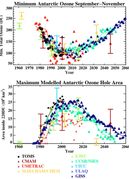
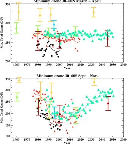
The results are also compared to determine the possible future behaviour of ozone, with an emphasis on the polar regions and mid-latitudes. All models predict eventual

15

ozone recovery, but give a range of results concerning its timing and extent. Differences in the simulation of gravity waves and planetary waves as well as model resolution are likely major sources of uncertainty for this issue. In the Antarctic, the ozone hole has probably reached almost its deepest although the vertical and horizontal extent of depletion may increase slightly further over the next few years. According to the model

20

results, Antarctic ozone recovery could begin any year within the range 2001 to 2008. For the Arctic, most models indicate that small ozone losses may continue for a few more years and that recovery could begin any year within the range 2004 to 2019. The start of ozone recovery in the Arctic is therefore expected to appear later than in the Antarctic in most models. Further, interannual variability will tend to mask the signal for

25

longer in the Arctic than in the Antarctic, delaying still further the date at which ozone recovery may be said to have started. In the longer term, the model results suggest that full recovery of ozone to 1980 levels is not expected in the Antarctic until about

ACPD

Full Screen / Esc

Print Version Interactive Discussion

c

EGS 2002

the year 2050. Earlier recovery to 1980 levels may be possible in the Arctic, but model differences are too large compared with the simulated changes to obtain a reliable date.

1. Introduction

Despite considerable research on the topic, the extent to which stratospheric change

5

can influence climate is only beginning to be understood. Before the discovery of the Antarctic ozone hole (Farman et al., 1985) it was thought that increases in the concen-tration of CO₂would cool the stratosphere and increase ozone (e.g. Groves and Tuck, 1980). More generally it is recognised that increases in the so-called well-mixed green-house gases (WMGHGs), which include CO₂, CH₄, N₂O and chlorofluorocarbons, cool

10

the stratosphere, although the vast majority arises through increases in CO₂amounts. In polar regions, an increase in WMGHGs may increase Polar Stratospheric Clouds (PSCs) and decrease ozone (Austin et al., 1992) via the same processes leading to the ozone hole (Solomon, 1986). Changes to the thermal structure of the stratosphere also affect the wind fields which determine the transport of ozone and the long-lived

15

species that chemically control ozone. Decreases in stratospheric ozone change tropo-spheric chemistry by increasing the amount of UV radiation reaching the troposphere, and also cool the troposphere as ozone is itself a greenhouse gas. Consequently, atmospheric chemistry and climate are coupled in important ways. Possibly one of the most extreme examples of this coupling is the effect of increasing WMGHGs on

20

Arctic ozone. Using a mechanistic model with reasonably comprehensive chemistry Austin et al. (1992) showed that a doubling of CO₂ concentrations, expected towards the end of the 21st century, could lead to severe Arctic ozone loss if large halogen abundances persisted until that time. On the other hand, the calculations of Pitari et al. (1992) showed only a slight reduction in Arctic ozone due to a CO₂doubling, while

25

again keeping halogen amounts fixed.

Since the early 1990s, the amendments to the Montreal protocol have resulted in 1037

ACPD

Full Screen / Esc

Print Version Interactive Discussion

c

EGS 2002

a considerable constraint on the evolution of halogen amounts and more recent cal-culations have been able to take this into consideration. For example, in a coupled chemistry-climate simulation, (Shindell et al., 1998a) specified currently projected con-centrations of halogens and WMGHGs and calculated much increased ozone deple-tion over the next decade or so, with severe ozone loss in the Arctic in some years. In

5

contrast, recent results from other models (Austin et al., 2000; Br ¨uhl et al., 2001; Na-gashima et al., 2002; Schnadt et al., 2002) indicate a relatively small change in Arctic ozone over the next few decades. The net effect on ozone and temperature is that due to both the increased radiative cooling from WMGHG increases and due to changes in downwelling (and adiabatic warming) from planetary wave drag. The latter changes

10

could decrease ozone if planetary wave activity decreases, thus enhancing the radia-tive signal, or if planetary wave activity increases, the radiaradia-tive signal could be damped or even reversed causing an increase in ozone. This illustrates one of the problems concerning future predictions: the simulation of the north polar stratospheric tempera-ture, and thus ozone, is complicated by the models’ ability to reproduce realistically the

15

dynamical activity of this region. The model results therefore crucially depend on the length of the numerical simulation and model configuration, such as spatial resolution, position of the model upper boundary, gravity wave drag scheme and the degree of coupling between the chemically active species and the radiation scheme. The fact that the results are model dependent emphasises that the various dynamical-chemical

20

feedback mechanisms in the atmosphere, as well as the dynamical coupling between troposphere and stratosphere, are not yet fully understood. These mechanisms are here explored by comparing specific diagnostics from a range of coupled chemistry-climate models. The primary interest is polar ozone and factors that control it, such as PSCs. Via transport, polar ozone also has an impact on middle latitudes which are

25

also considered briefly.

In Sect. 2, the three-dimensional (3-D) coupled chemistry-climate models used in this comparison are described. The emphasis is on coupled models in which increases in WMGHGs give rise, directly or indirectly, to changes in the concentrations of

con-ACPD

Full Screen / Esc

Print Version Interactive Discussion

c

EGS 2002

stituents, especially ozone. These changes then react back on the model climate via the model radiation scheme. In Sect. 3, several factors known to affect model pre-dictions of ozone are investigated using, as indicated above, specific diagnostics de-signed to illustrate model differences and uncertainties. These diagnostics are com-pared amongst the models and with observations. Having established model strengths

5

and weaknesses, their results are assessed in Sect. 4, to try to provide a consensus on the likely trend in future ozone. Conclusions are drawn in Sect. 5.

2. Models used in the comparisons

Climate models have in the past been run with fixed WMGHGs for both present and doubled CO₂ with the investigation of the subsequent ‘equilibrium climate’. Several

10

coupled chemistry-climate runs have followed this route with multi-year ‘timeslice’ sim-ulations applicable to WMGHG concentrations for specific years (e.g. Rozanov et al., 2001; Schnadt et al., 2002; Pitari et al., 2002; Steil et al., 2002). Other climate simulations have involved transient changes in the WMGHGs, and several coupled chemistry-climate simulations have followed this pattern (Shindell et al., 1998a; Austin

15

2002; Nagashima et al., 2002). The advantage of transient experiments is that the detailed evolution of ozone can be determined in the same way that it is likely to oc-cur (in principle) in the atmosphere, albeit with some statistical error. The impact of interannual variability can be assessed by determining this variability over, e.g. a 10-year period. Comparisons with observations are more direct since both atmosphere

20

and model cover the period when WMGHGs and halogens are changing to the same extent. Timeslice simulations need a sufficient duration (at least 10 and preferably 20 years) to allow the interannual variability to be determined but in principle, 20-year eval-uations of the same conditions may have less variability than the atmosphere in which halogens may be changing rapidly. Timeslice runs also have the advantage that

sev-25

eral realisations of the same year are available, from which future predictions can be assessed. However, in practice this may be of less value than examining the behaviour

ACPD

Full Screen / Esc

Print Version Interactive Discussion

c

EGS 2002

of different models, since a given model will tend to have systematic errors. Both tran-sient simulations and timeslice simulations are here used, to bring together the best of both sets of simulations.

The models used in the comparisons are indicated in Table 1, in order of decreasing horizontal resolution. All the models have a comprehensive range of chemical reactions

5

except that in the GISS model the chemistry is parameterized. ULAQ is the only model with a substantial aerosol package and has diurnally averaged chemistry. This model has been run in timeslice mode. Of the other models run in this mode, CMAM and

MAECHAM/CHEM have a high upper boundary (0.01 hPa and above), while UIUC and E39/C have a much lower upper boundary (1 hPa and below). UMETRAC, CCSR/NIES

10

and GISS have been run in transient mode, although the extra cost of the UMETRAC model has reduced the total integration time compared with the other two models. Brief summaries of the models follow.

2.1. Model descriptions

UMETRAC

15

The Unified Model with Eulerian TRansport And Chemistry is based on the Meteo-logical Office’s Unified Model (UM), which has been used in the Intergovernmental Panel on Climate Change (IPCC) assessments (e.g. IPCC, 2001). UMETRAC has 64 vertical levels, from the ground to 0.01 hPa, and includes a coupled stratospheric chemistry scheme involving 13 advected tracers (O₃, HNO₃, N₂O₅, HNO₄, HCl(g+s),

20

HOCl, ClONO₂, HOBr, HBr, BrONO₂, H₂O₂, H₂CO, Tracer-1). Tracer-1 is used to pa-rameterize the long-lived species and families H₂O, CH₄, Cl_y, Br_y, H₂SO₄ and NO_y, where Cl_y = Cl + ClO + HCl(g+s) + HOCl + ClONO₂ + 2Cl₂O₂ + BrCl, Br_y = Br + BrO+ HBr + BrONO₂ + HOBr + BrCl, and NO_y = NO + NO₂ + NO₃ + HNO₃(g+s) + 2N2O5 + HNO4 + ClONO2 + BrONO2. In the above (g+s) is used to denote the 25

sum of concentrations is the gas (g) and solid (s) phases. A simplified sedimentation scheme is included and the PSC scheme is based on liquid ternary solutions (LTS) and ice or nitric acid trihydrate (NAT) and water ice. The photochemistry therefore

ex-ACPD

Full Screen / Esc

Print Version Interactive Discussion

c

EGS 2002

plicitly includes all the major processes affecting stratospheric ozone. Reaction rates are taken from DeMore et al. (1997) and Sander et al. (2000). Sea surface temper-atures and sea ice are specified from observations or from simulations of a coupled ocean-atmosphere version of the model. The dynamics is available using Rayleigh friction as standard to decelerate the jet or with a non-orographic gravity wave drag

5

(gwd) scheme. Halogen amounts are specified according to WMO (1999), Tables 1–2, and the greenhouse gas concentrations (CO₂, CH₄and N₂O) are specified according to IPCC scenario IS92a (IPCC, 1992). Simulations have been completed for the peri-ods 1979–2020 (Rayleigh friction) and 1975–2020 (non-orographic gwd). The results of the model for the Rayleigh friction calculations covering the period 1980–2000 are

10

described in Austin (2002).

CMAM (Canadian Middle Atmosphere Model) is an extension of the Canadian Centre

for Climate Modelling and Analysis (CCCma) spectral General Circulation Model up to 0.0006 hPa, roughly 100 km altitude (Beagley et al., 1997). The version used here

15

has a T32 spectral truncation and 65 vertical levels. The model includes a full repre-sentation of stratospheric chemistry with all the relevant catalytic ozone loss cycles de Grandpr ´e et al., 1997). There are 31 non-advected species and 16 advected species and families HNO₄, HBr, CO, H₂, CH₃Br, CH₄, N₂O, H₂O, CFC-11, CFC-12, O_x (= O(1D) + O(3P) + O₃), NO_x (= NO + NO₂ + NO₃ + 2N₂O₅), ClO_x (= ClO + OClO

20

+ HOCl + Cl + ClONO2 + 2Cl2O2 + 2Cl2 + HCl(g+s)), BrOx (= Br + BrO + BrCl +

BrONO₂+ HOBr), HO_x(= OH + HO₂+ H + 2H₂O₂), and HNO₃(g+s). Chemical trans-port is accomplished using spectral advection. Heterogeneous reactions are included for sulphate aerosols, LTS, and water ice, without sedimentation. There is currently no parameterization of NAT PSCs, or of any associated denitrification. PSC threshold

25

temperatures are not adjusted to compensate for temperature biases. Chemical reac-tion rates follow DeMore et al. (1997) and Sander et al. (2000). The chemistry is fully interactive with the radiation code (de Grandpr ´e et al., 2000). For these runs, gravity-wave drag is parameterized with the McFarlane orographic scheme and the Hines

ACPD

Full Screen / Esc

Print Version Interactive Discussion

c

EGS 2002

non-orographic scheme (McLandress, 1998; Beagley et al., 2000). The time-slice ex-periments are performed for 12 years, with the first year discarded. For the 1980 and 2000 runs, WMGHGs (CO₂, CH₄and N₂O) and halogens are specified from observa-tions, and the sea surface temperatures and sea-ice distributions are taken from Shea et al. (1990). For the 2045 run, WMGHGs are taken from the IPCC IS92a scenario

5

while the halogens are set to 1980 levels; sea-surface temperatures and sea-ice dis-tributions are altered according to the anomalies predicted from a transient simulation with the CCCma coupled climate model (Boer et al., 2000).

MAECHAM/CHEM is a coupled chemistry-climate model based on the MA-ECHAM4

10

climate model. The chemistry module (Steil et al., 1998) adopts the ‘family’ technique allowing timesteps to be as large as 45 min and includes reactive chlorine, nitrogen and hydrogen, and methane oxidation. Photolysis rates are calculated on-line using the fast and accurate scheme of Landgraf and Crutzen (1998) to account for varying clouds and overhead ozone. Heterogeneous reactions on NAT and ice PSCs, and on

15

sulphate aerosol are included, as well as sedimentation of ice PSC particles. Since it is assumed that ice grows on NAT particles, this accounts to some extent for den-itrification if it is cold enough for ice. NAT PSCs are calculated from the model tem-perature, H₂O and HNO₃ using the formulae of Hanson and Mauersberger (1988), without assuming a nucleation barrier arguing that subgrid scale temperature

fluctua-20

tions produce the required supercooling. The gravity wave parameterization consists of two parts, separately representing momentum flux deposition due to orographic gravity waves and a broad band spectrum of nonorographic gravity waves (Manzini and Mc-Farlane, 1998). A modified version of the McFarlane (1987) parameterization is used to account for the orographic gravity wave drag. Chemical species are advected using

25

the fluxform semi-Lagrangian transport scheme of Rasch and Lawrence (1998). For the time slice experiments the model is integrated about 22 years (including spinup) using fixed surface mixing ratios of source gases (WMO, 1999) and ten years aver-age seasonal sea surface temperture distributions based on Hadley Centre data. For

ACPD

Full Screen / Esc

Print Version Interactive Discussion

c

EGS 2002

the simulations of future conditions, the average sea surface temperatures have been taken from the transient climate simulation of Roeckner et al (1999).

E39/C

A detailed description of the chemistry-climate model E39/C, also known as

5

ECHAM4.L39(DLR)/CHEM, has been given by Hein et al. (2001), who also discussed

the main features of the model climatology. The model horizontal resolution is T30 with a corresponding Gaussian transform latitude-longitude grid of mesh size 3.75◦× 3.75◦ on which model physics, chemistry, and tracer transport are calculated. The model has 39 layers from the surface to the top layer centred at 10 hPa (Land et al., 1999) and

10

has particularly high resolution near the tropopause. A parameterization for orographic gravity wave drag (Miller et al., 1989) is employed, but the effects of non-orographic gravity waves are not considered. The chemistry module CHEM (Steil et al., 1998, updated Hein et al., 2001) uses reaction rate coefficients from DeMore et al. (1997) and is based on the family concept, containing the most relevant chemical compounds

15

and reactions necessary to simulate upper tropospheric and lower stratospheric ozone chemistry, including heterogeneous chemical reactions on PSCs and sulphate aerosol, as well as tropospheric NO_x− HOx− CO − CH4− O3chemistry. The advected tracers

are CH₄, HCl, H₂O₂, CO, CH₃O₂H, ClONO₂, O_x (= O(1D)+ O(3P) + O₃), NO_x (= N + NO + NO2 + NO3 + 2N2O5 + HNO4), ClOx (= Cl + ClO + HOCl), HNO3 + NAT 20

and H₂O+ ICE. Physical, chemical, and transport processes are calculated simultane-ously at each time step, which is fixed to 30 min. The PSCs in the model are based on NAT and ice amounts depending on the temperature and the concentration of HNO₃ and H₂O (Hanson and Mauersberger, 1988). A nucleation barrier is prescribed to ac-count for the observed super-saturation of NAT-particles (Schlager et al., 1990; Peter

25

et al., 1991; Dye et al., 1992). A simplified scheme for the sedimentation of NAT and ice particles is applied. Stratospheric sulphuric acid aerosol surface areas are based on background conditions (WMO, 1992, Chapter 3) with a coarse zonal average. Sea surface temperature and sea ice distributions are prescribed for the various time slices

ACPD

Full Screen / Esc

Print Version Interactive Discussion

c

EGS 2002

according to the greenhouse gas driven transient climate change simulations of Roeck-ner et al. (1999).

UIUC (University of Illinois at Urbana-Champaign) is a global-scale grid-point General

Circulation Model with interactive chemistry (Yang et al., 2000; Rozanov et al., 2001).

5

The model horizontal resolution is 4◦latitude and 5◦longitude, with 24 layers spanning the atmosphere from the surface to 1 hPa. The chemical-transport part of the model simulates the time-dependent three-dimensional distributions of 42 chemical species (O₃, O(1D), O(3P), N, NO, NO₂, NO₃, N₂O₅, HNO₃, HNO₄, N₂O, H, OH, HO₂, H₂O₂, H₂O, H₂, Cl, ClO, HCl, HOCl, ClONO₂, Cl₂, Cl₂O₂, CF₂Cl₂, CFCl₃, Br, BrO, BrONO₂,

10

HOBr, HBr, BrCl, CBrF₃, CH₃Br, CO, CH₄, CH₃, CH₃O₂, CH₃OOH, CH₃O, CH₂O, and CHO), which are determined by 199 gas-phase and photolysis reactions. The model also takes into account 6 heterogeneous reactions on and in sulphate aerosol and polar stratospheric cloud particles. The chemical solver is based on the pure implicit iterative Newton-Raphson scheme (Rozanov et al., 1999). The reaction coefficients are taken

15

from DeMore et al. (1997) and Sander et al. (2000). Photolysis rates are calculated at every chemical step using a look-up-table (Rozanov et al., 1999). The advective trans-port of species is calculated using the hybrid advection scheme proposed by Zubov et al. (1999). A simplified scheme is applied for the calculation of the PSC particles (NAT and ice) formation and sedimentation. Sea surface temperature and sea ice

dis-20

tributions are prescribed from the AMIP-II monthly mean distributions, which are the averages from 1979 through 1996 (Gleckler, 1996). The orographic scheme of Palmer et al. (1986) is used to parameterize gravity wave drag. In this paper the results of a 15-year long control run of the model will be considered. The climatology of this run has been presented by Rozanov et al. (2001).

25

CCSR/NIES

An overview of the CCSR/NIES (Center for Climate System Research/National Institute for Environmental Studies) GCM (General Circulation Model) with an interactive

strato-ACPD

Full Screen / Esc

Print Version Interactive Discussion

c

EGS 2002

spheric chemistry module has been described in Takigawa et al. (1999), and some updates for the present integration are given by Nagashima et al. (2002). A horizontal resolution of T21 (longitude × latitude ' 5.6◦× 5.6◦) is employed and the vertical do-main extends from the surface to about 0.01 hPa with 34 layers. Orographic gwd is parameterized following McFarlane (1987), but non-orographic gwd is not included. In

5

the model, 19 species and 5 chemical families are explicitly transported: CH₄, N₂O, H₂O₂, H₂O(g+s), HNO₃+ NAT, HNO₄, N₂O₅, ClONO₂, HCl, HOCl, Cl₂, ClNO₂, CCl₄, CFC11, CFC12, CFC113, HCFC22, CH₃Cl, CH₃CCl₃, O_x, HO_x (= H + OH +HO₂), NO_x(= N + NO +NO₂ + NO₃), ClO_x (= Cl + ClO + ClOO + Cl₂O₂), NO_y and Cl_y. The amount of NAT and ice PSCs are calculated using the relationship of Hanson and

10

Mauersberger (1988) and of Murray (1967), respectively. As in E39/C, a nucleation barrier is also assumed. Reaction rate coefficients are taken primarily from DeMore et al. (1997) and Sander et al. (2000). A 65-year transient integration was performed for the period 1986–2050 including the trends of chlorine-containing substances (WMO, 1999, Table 12-2) and those of greenhouse gases (Also WMO, 1999, Table 12-2, very

15

similar to IPCC scenario IS92a, IPCC, 1992). The expected sea surface temperature variation, separately calculated by the CCSR/NIES coupled ocean-atmospheric GCM, is also applied.

GISS

20

The model used here is a version of the Goddard Institute for Space Studies (GISS) stratospheric climate model which has 8◦×10◦horizontal resolution, and 23 vertical lay-ers extending up into the mesosphere (top at 0.002 hPa, ∼ 85 km) (Rind et al., 1988a, b). This atmospheric model is coupled to a mixed-layer ocean, allowing sea surface temperatures to respond to external forcings. A gravity wave parameterization is

em-25

ployed in the model in which the temperature and wind fields in each grid box are used to calculate gravity wave effects due to wind shear, convection, and topography. For the runs described here, the mountain drag was set to one quarter the original value which gives a better reproduction of observed temperatures in the polar lower stratosphere of

ACPD

Full Screen / Esc

Print Version Interactive Discussion

c

EGS 2002

each hemisphere during their respective winter and spring periods. The model includes a simple parameterization of the heterogeneous chemistry responsible for polar ozone depletion (Shindell et al., 1998a). Chlorine activation takes place whenever tempera-tures fall below 195 K. Ozone depletion is then calculated at each location with active chlorine and sunlight using the reaction rates of DeMore et al. (1997). An additional

5

contribution of 15% from bromine chemistry is also included. When heterogeneous processing ceases, chlorine deactivation follows two-dimensional model-derived rates Shindell et al., 1998b). Ozone recovery rates are parameterized so that ozone losses are restored based on the photochemical lifetime of ozone at each altitude. Changes in ozone transport are not included interactively, but are calculated after the model runs

10

and included in the results shown here. The model was run with increasing greenhouse gases starting in 1959 and continuing until 2067. Greenhouse gas trends were based on observations through 1985, and subsequently followed the IPCC projections IS92a (IPCC, 1992), though the observed trends since 1985 have shown somewhat slower increases.

15

ULAQ

The University of L’Aquila (ULAQ) model is a low-resolution coupled chemistry-climate model, which has been extensively used in the IPCC assessment (IPCC, 2001). The chemical-transport module has a resolution of 10◦× 20◦ in latitude-longitude. There

20

are 26 log-pressure levels, from the ground to about 0.04 hPa, giving an approximate vertical resolution of 2.8 km. Dynamical fields (streamfunction, velocity potential and temperature) are taken from the output of a spectral GCM (Pitari et al., 2002). Verti-cal diffusion is used to simulate those processes not explicitly included in the model such as the effect of breaking gravity waves. See Pitari et al. (1992) and Pitari et

25

al. (2002) for further details of the model. The Chemical Transport Model (CTM) and GCM are coupled via the dynamical fields and via the radiatively active species (H₂O, CH₄, N₂O, CFCs, O₃, NO₂, and aerosols). All chemical species are diurnally averaged. The medium and short-lived chemical species are grouped into families: O_x, NO_x, NO_y

ACPD

Full Screen / Esc

Print Version Interactive Discussion

c

EGS 2002

(= NO_x+ HNO₃), HO_x, CHO_x, Cl_y, Br_y, SO_xand aerosols. The long-lived and surface-flux species in the model are N₂O, CH₄, H₂O, CO, NMHC, CFCs, HCFCs, halons, OCS, CS₂, DMS, H₂S, SO₂for a total of 40 transported species (plus 57 aerosol size categories) as well as 26 species at photochemical equilibrium. All photochemical data are taken from DeMore et al. (1997), including the most important heterogeneous

5

reactions on sulphate and PSC aerosols. The ULAQ model also includes the most im-portant tropospheric aerosols. The size distribution of sulphate (both tropospheric and stratospheric) and PSC aerosols, treated as NAT and water ice, are calculated using a fully interactive and mass conserving microphysical code for aerosol formation and growth. Denitrification and dehydration due to PSC sedimentation are calculated

ex-10

plicitly from the NAT and ice aerosol predicted size distribution. WMGHG and halogen scenarios are taken from WMO (1999). Changes in surface fluxes of CO, NO_x, non-methane hydrocarbons, SO_xand carbonaceous aerosols are taken from IPCC (2001). Climatological sea surface temperatures (SSTs) are used for present day conditions, and a simple heat source model is used to estimate the change in SSTs for future

15

conditions.

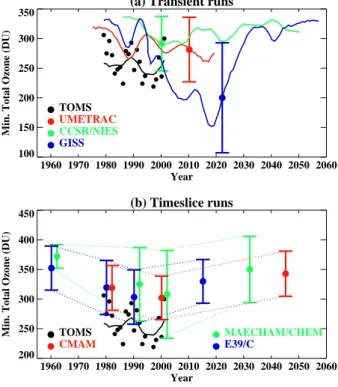
2.2. Model ozone climatologies for the current atmosphere

To put the subsequent model results into context, we first compare the ozone clima-tologies from the different models during spring with the corresponding satellite ob-servations for the years 1993–2000 (see Rozanov et al., 2001 for a description of the

20

data included). The geographical distribution of the monthly mean total ozone over the northern hemisphere in March and over the southern hemisphere in October are presented in Figs. 1 and 2 for the data and participating models. The hemispheric area weighted total ozone and pattern correlation coefficients between the observed and simulated total ozone fields are presented in Table 2. The GISS model results are

25

not shown in this section, as the chemistry parameterization is a perturbation from the observed climatology.

In the northern hemisphere (Fig. 1), all the models simulate the position and in-1047

ACPD

Full Screen / Esc

Print Version Interactive Discussion

c

EGS 2002

tensity of the primary total ozone maximum reasonably well. However, UMETRAC,

CCSR/NIES, E39/C and CMAM models slightly overestimate the extension of the ozone

maximum area. In these models the area where total ozone is higher than 425 DU covers a substantial part of Siberia and spreads to northern Canada. Total ozone in

MAECHAM/CHEM is higher than observed values over the entire hemisphere. The

5

area of ozone maximum in the UIUC and ULAQ models extends to the Pacific sec-tor, which implies an underestimated intensity of the Aleutian highs in the stratosphere. This dynamical feature also leads to the equatorward shift of the area with elevated total ozone in the Pacific sector. The CCSR/NIES model simulates very well the magnitude of the primary maximum, although its position is slightly shifted to the west. This shift,

10

and the shape of the 400 DU contour imply that the intensity of the Aleutian maximum in the CCSR/NIES model is overestimated. The simulated position and magnitude of the elevated total ozone over northern Canada are in good agreement with observa-tions. However, in most of the participating models this area is shifted to the north and its magnitude is slightly overestimated, while the UIUC and ULAQ models tend to shift

15

this area to the south. In agreement with the observations the area with rather low total ozone appears in UIUC, CCSR/NIES, MAECHAM/CHEM and E39/C models just over the North Pole reflecting the position of the Polar vortex. However, this feature is not present in the UMETRAC, ULAQ and CMAM total ozone maps. Table 2 shows that the overall performance of all the models in March over the northern hemisphere

20

is reasonably good. The pattern correlation with observed data is very high for

UME-TRAC, CCSR/NIES, E39/C, CMAM and MAECHAM/CHEM models (R2 > 0.95) but a

lower correlation occurs for the UIUC and ULAQ models partially because of the un-derprediction in the strength of the Aleutian high. All the models overestimate the area weighted hemispheric total ozone, by on average 7.2%.

25

In the southern hemisphere (Fig. 2), the overall agreement between simulated and observed total ozone in October is similar as in the northern hemisphere, as indicated by the pattern correlations (Table 2). UMETRAC, CCSR/NIES, MAECHAM/CHEM,

ACPD

Full Screen / Esc

Print Version Interactive Discussion

c

EGS 2002

total ozone surplus comes from slightly higher total ozone in the tropics and from sub-stantial overestimation of the magnitude of the total ozone maximum over the middle latitudes. For example the total ozone exceeds 475 DU in the UMETRAC results, 450 DU in MAECHAM/CHEM and 425 DU in the CCSR/NIES, and CMAM results, while in the observations the total ozone peak just exceeds 375 DU. From these results we can

5

conclude that the meridional transport and wave forcing are overestimated by these models. In contrast the E39/C and UIUC models, which are the two models with the lowest upper boundary, match the observed total ozone very closely. The position of the total ozone maximum over middle-latitudes is also shifted from the Australian sector to the Indian Ocean sector in UMETRAC and CCSR/NIES models and to the

10

Pacific Ocean sector in the UIUC model. The position and magnitude of the ozone hole over the South Pole is well reproduced by the models, implying that the amount of PSCs during the spring season and chemical ozone destruction are reasonably well captured by the chemical routines. This is discussed further in Sects. 3.2 and 4.4.

3. Model uncertainties 15

3.1. Temperature biases

Many climate models without chemistry but with a fully resolved stratosphere have a cold bias of the order of 5–10 K in high southern latitudes in the lower stratosphere, suggesting that the residual circulation is too weak (Pawson et al., 2000), i.e. there is too little downwelling in polar latitudes and too little upwelling in lower latitudes. This

20

temperature bias could have a significant impact on model heterogeneous chemistry, and enhance ozone destruction. The ‘cold pole problem’ extends to higher levels in the stratosphere and by the thermal wind relation gives rise typically to a polar night jet that is too strong and which has an axis that does not slope with height, whereas in the observations the polar night jet axis slopes with height towards the equator in

25

the upper stratosphere. The weaker jet and slope of the axis allow waves to propagate 1049

ACPD

Full Screen / Esc

Print Version Interactive Discussion

c

EGS 2002

into higher latitudes and maintain higher polar temperatures. A potentially important component of climate change is whether these waves increase in amplitude with time since this will likely affect the evolution of ozone: see Sect. 3.4. A practical solution for those models with a cold bias is to adjust the temperatures in the heterogeneous chemistry (e.g. Austin et al., 2000) so that the heterogeneous chemistry is calculated

5

using realistic temperatures. The strong polar night jet is also associated with a vortex that breaks down later in the spring, particularly in the southern hemisphere. In a chemistry-climate model this can lead to a longer lasting ozone hole. Adjusting model PSC threshold temperatures to allow for model temperature bias cannot solve this problem.

10

Recently the development of non-orographic gravity wave drag (gwd) schemes for climate models (Medvedev and Klaassen, 1995; Hines, 1997; Warner and McIntyre, 1999) has resulted in a significant reduction in the cold pole problem relative to sim-ulations that rely on Rayleigh friction to decelerate the polar night jet (e.g. Manzini and McFarlane, 1998). Two of these schemes have also been shown to produce a

15

quasi-biennial oscillation (QBO) when run in a climate model (Scaife et al., 2000). The latest versions of several coupled chemistry-climate models now employ such schemes: CMAM uses the Medvedev-Klaassen scheme (Medvedev et al., 1998) or the Hines scheme (McLandress, 1998); the latest version of UMETRAC uses the Warner and McIntyre scheme; and MAECHAM/CHEM uses the Hines scheme (Manzini et al.,

20

1997). The GISS GCM has used a non-orographic gravity wave drag scheme for many years (Rind et al., 1988a, b), which is able to reproduce high latitude temperatures reasonably well (Shindell et al., 1998b) but does not simulate a QBO in the tropics.

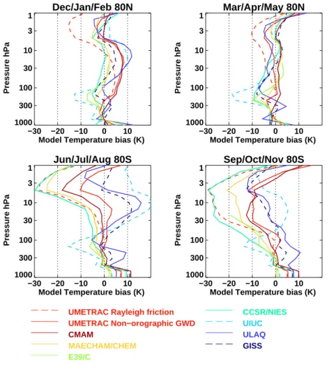
Figure 3 shows model temperature biases as a function of height for 80◦N and 80◦S for the winter and spring seasons. To determine the biases, a 10-year temperature

25

climatology determined from data assimilation fields (Swinbank and O’Neill, 1994) was subtracted from the mean model temperature profiles applicable to the 1990s. The UKMO temperatures are considered to be about 2 K too high at low temperatures (e.g. Pullen and Jones, 1997) but this is somewhat smaller than typical model biases.

ACPD

Full Screen / Esc

Print Version Interactive Discussion

c

EGS 2002

The upper stratospheric cold pole problem is particularly noticeable in the south in the UMETRAC (with Rayleigh friction), CCSR/NIES and E39/C (which also use Rayleigh friction) and MAECHAM/CHEM results. With a non-orographic gwd scheme the tem-perature biases reduce considerably and both CMAM and UMETRAC have very similar results in the seasons analysed. In the UIUC, GISS and ULAQ models a warm bias is

5

present in the middle stratosphere in winter. For the latter models, which have lower horizontal resolution than the other five, the biases may be a result of the need to adjust physical parameterizations to obtain improved climatologies and that such adjustments are not always suitable for all seasons. The ULAQ model, for example, includes vertical diffusion, in addition to Rayleigh friction. The results of the MAECHAM/CHEM model,

10

which uses the Hines non-orographic gwd scheme, are only a slight improvement on the Rayleigh friction results of UMETRAC and CCSR/NIES and are similar to the re-sults of E39/C which has equivalent physics, but does not have a non-orographic gwd scheme. Nonetheless, Manzini et al. (1997) indicated that the temperature biases in the core climate model are larger when non-orographic gwd is not included.

15

At 80◦N temperature biases are generally somewhat smaller than at 80◦S and for some models are positive at some levels. The northern lower stratospheric tempera-ture biases would generally lead to insufficient heterogeneous ozone depletion in early winter but excessive ozone depletion in the more important spring period. In the south-ern hemisphere, spring cold biases could lead to more extensive PSCs than observed

20

and delayed recovery in Antarctic ozone.

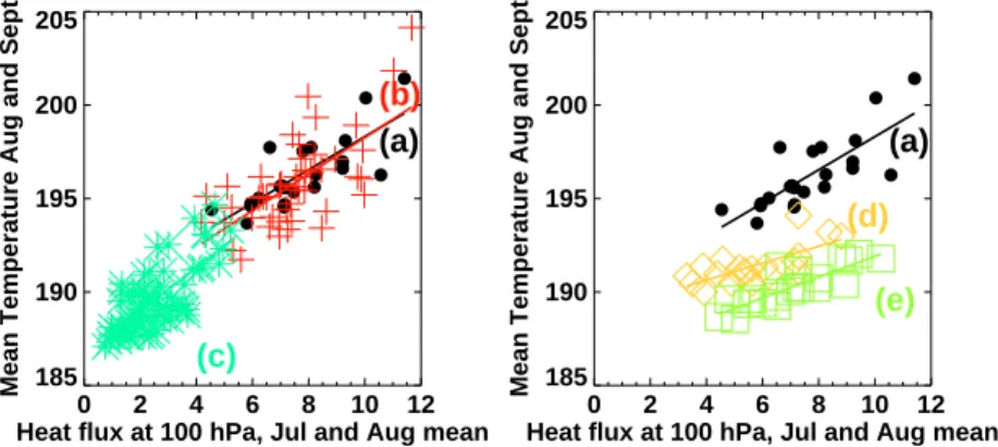
Newman et al. (2001) showed that the lower stratospheric temperature is highly cor-related with the lower stratospheric heat flux v0T0 slightly earlier in the year. The heat flux provides a measure of the wave forcing from the troposphere, and in Fig. 4, the heat flux at 100 hPa averaged over the domain 40◦–80◦N for January and February is

25

plotted against temperature averaged over the domain 60◦–90◦N at 50 hPa for Febru-ary and March. Similar results for the southern hemisphere are shown in Figure 5. Newman et al. choose the period of the temperature average as 1–15 March, which maximises the correlation coefficient between the two variables at 0.85. However, here

ACPD

Full Screen / Esc

Print Version Interactive Discussion

c

EGS 2002

we choose a longer period for the temperature average to smooth over any model and atmospheric transients. This reduces the correlation coefficient for NCEP data only slightly, to 0.77 (0.78 in the south). Table 3 shows the correlation coefficient (R) be-tween the two variables. β is the gradient of the lines in Figs. 4 and 5, and T₀ is the temperature intercept at zero flux. T₀ indicates the radiative equilibrium temperature,

5

including a contribution from small scale waves not represented in the heat flux (e.g. Newman et al., 2001).

In the north (Fig. 4), the model results are for the most part in reasonable agreement with the observations, although the model correlation coefficients vary in the range 0.52 to 0.79. Model horizontal resolution may have significantly affected the results: in

10

general the model regression lines are less steep (smaller β in Table 3) as the model resolution decreases. This could be because while low-resolution models can capture the low-amplitude wave, small heat flux case, they may have more difficulty captur-ing the large heat flux case with its possibly significant potential enstrophy cascade to larger wavenumbers. However, this covers a broad spectrum of results. For example,

15

CMAM simulates a wide range of heat fluxes consistent with observations but the func-tional relationship with temperature is highly sensitive to a single year’s data. Removal of the single point corresponding to the highest heat flux, increases the correlation co-efficient to 0.71 and increases β to 1.12, much closer to that expected on the basis of the model resolution. This implies that the 10-year CMAM run is too short to give fully

20

meaningful results in the northern hemisphere for this diagnostic. The performance of the models might also depend on the dissipation that the models have at short spatial scales, although this is more difficult to compare.

In the southern hemisphere (Fig. 5) the correlation coefficients cover the range 0.48 to 0.86, wider than in the north. T₀is considerably lower, probably due to lower ozone

25

amounts, and all the models agree well with the observed T₀. For the timeslice experi-ments (e.g. MAECHAM/CHEM) T₀decreased from the 1960 results (not shown) to the 1990 results due to the WMGHG increase and ozone depletion. The values of β are also generally much smaller in the southern hemisphere, except for the CCSR/NIES

ACPD

Full Screen / Esc

Print Version Interactive Discussion

c

EGS 2002

and CMAM models. For the CCSR/NIES model, the heat fluxes are much lower than observed, as they are in the northern hemisphere, consistent with a very strong polar vortex. The CMAM results are in reasonable agreement with observation for the value of β and the comparison with the northern hemisphere reflects the shortness of the record, as indicated above. Comparison of the UMETRAC results with Rayleigh

fric-5

tion and with non-orographic gwd indicate that the latter can significantly improve the temperature-heat flux relationship.

3.2. The simulation of polar stratospheric clouds

During the last few years, considerable progress has been made regarding the un-derstanding of PSCs and the associated heterogeneous chemical reactions. Some of

10

these developments are discussed in Carslaw et al. (2001) and WMO (2002), Chapter 3. They include the observation of many different types of PSCs, both liquid and solid forms, and the laboratory measurement of a wide range of chemical reaction rates as summarised in Sander et al. (2000). Coupled chemistry-climate models have a variety of PSC schemes with and without sedimentation, but as indicated in Sect. 3.1, some

15

models have large climatological biases in the polar regions. If the models are to pro-duce accurate simulations of ozone depletion, the temperature field must give realistic distributions near the PSC temperature threshold. So that common ground can be established between models, we here use the temperature at 50 hPa as an indicator, hence ignoring the impact of HNO₃and sulphate concentrations on the determination

20

of PSC surface areas.

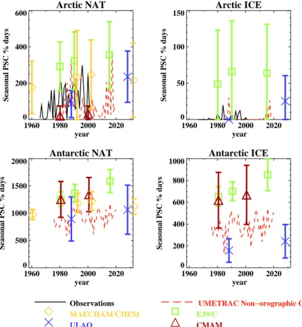
Following Pawson and Naujokat (1997) and Pawson et al. (1999), Fig. 6 shows for each of the participating models and observations the time integral throughout the winter of the approximate PSC area at 50 hPa, as given by the areas within the 195 K and 188 K temperature contours. This is the quantity ˜A_τ indicated in Fig. 9 of Pawson

25

et al. (1999), but without the normalisation factor of 1/150, for τ_NAT = 195 K and τ_ICE = 188 K. ˜A_τis here measured in terms of the fraction of the hemisphere covered in the ice amount in the Arctic, ˜A_τ varies dramatically between zero (ULAQ and CMAM models,

ACPD

Full Screen / Esc

Print Version Interactive Discussion

c

EGS 2002

not shown) and 70 in units of % of the hemisphere times days and the models have large interannual variability. Arctic NAT also covers a large range, both for different models and in the interannual variability for each simulation. In accordance with their temperature biases, several models have larger areas of NAT than are typically derived from observations. The ULAQ PSCs are in good agreement with observations, despite

5

a slight temperature bias, while UMETRAC and CMAM have lower PSCs than are derived from observations. In the Antarctic most models have much lower fractional interannual variation, but again the results for separate models cover an exceedingly large range for the ice amount. The implications for ozone on the differences between the models is discussed further in Sect. 4.4.

10

The sedimentation of PSC particles is now thought to be important in polar ozone depletion (e.g. Waibel et al., 1999), but is absent from many coupled chemistry-climate models. Using a 3-D model without transport, Waibel et al. (1999) suggested that cooling associated with greenhouse gas increases may lead to higher ozone depletion than if sedimentation were ignored. There are many practical difficulties associated

15

with incorporating sedimentation in climate models. The full details, including divid-ing the particles into different sized bins (e.g. Timmreck and Graf, 2000), cannot be readily simulated in most models as this would require the transport of particles cov-ering a large number of size ranges, which may exceed the total number of tracers transported. While the ULAQ model (Pitari et al., 2002) is able to simulate this level

20

of complexity, the model resolution is somewhat coarse (see Table 1). Most models therefore adopt some extremely simplified procedures. For example in the UMETRAC model (Austin, 2002) sedimentation is assumed to occur for NAT or ice particles of fixed size. The vertical transport equation is solved locally to give a sedimented field which is not explicitly advected horizontally but is tied to the field of a conserved horizontal

25

tracer. Other models (e.g. Egorova et al., 2001; Hein et al., 2001; Pitari et al., 2002) transport the sedimented field in more detail, but the accuracy of this transport may be limited by model spatial resolution, and whether it can treat small scale features with high enough precision. Recently, the presence of large, nitric acid containing

parti-ACPD

Full Screen / Esc

Print Version Interactive Discussion

c

EGS 2002

cles exceeding 10 µm in diameter has been detected (Fahey et al., 2001) in the lower stratosphere. However, models have only just started to take the production of these particles into account (Carslaw, personal communication, 2002), although they may have an important impact on ozone depletion.

3.3. The transport of constituents

5

There is strong evidence from a number of modelling studies (Garcia and Boville, 1994; Shepherd et al., 1996; Lawrence, 1997; Austin et al., 1997; Rind et al., 1998; Beagley et al., 2000) that the position of the model upper boundary can play a significant role in influencing transport and stratospheric dynamics due to the ‘downward control princi-ple’ (Haynes et al., 1991). The sensitivity of the dynamical fields to the position of the

10

upper boundary may be more when using non-orographic gwd schemes than when Rayleigh friction is used, although if all the non-orographic gwd that is produced above the model boundary is placed instead in the top model layer, assuming that the upward propagating waves are not simply absorbed in the top layer, this sensitivity reduces (Lawrence, 1997). Model simulations with an upper boundary as low as 10 hPa have

15

been completed (e.g. Hein et al., 2001; Schnadt et al., 2002; Dameris et al., 1998). Schnadt et al. (2002) show the meridional circulation of the DLR model and this gives the expected upward motion from the summer hemisphere and downward motion over the winter hemisphere, although modeled meridional circulations are known to extend into the mesosphere (e.g. Butchart and Austin, 1998). Schnadt et al. (2002) argue that

20

it is less important for total ozone to have a high upper boundary, but more important to have high resolution in the vicinity of the tropopause. At present the evidence appears ambiguous: for example in the total ozone presented by Hein et al. (2001) insufficient ozone is transported to the North Pole, but there is excessive subtropical ozone trans-port. This could be related to the cold pole problem, rather than the position of the

25

upper boundary. While the transport effect on ozone is direct, other considerations are the transport of long-lived tracers such as NO_y and water vapour which have a pho-tochemical impact on ozone. Consequently, it is generally recognised that the upper

ACPD

Full Screen / Esc

Print Version Interactive Discussion

c

EGS 2002

boundary should be placed at least as high as 1 hPa (e.g. Rozanov et al., 2001; Pitari et al., 2002) with many models now placing their boundary at about 0.01 hPa (e.g. Shindell et al., 1998a; Austin et al., 2001; Steil et al., 2002; Nagashima et al., 2002). In comparison, CMAM (de Grandpr ´e et al., 2000) has an upper boundary somewhat higher (c. 0.0006 hPa) to allow a more complete representation of gwd to reduce the

5

cold pole problem (Sect. 3.1) and to simulate upper atmosphere phenomena.

The differences in transport can be assessed by investigating the Brewer-Dobson circulation computed for the individual models. An indicator of the circulation is given by the residual mean meridional circulation

v∗= v − ∂ ∂p v0θ0 ∂θ/∂p ! , 10 ω∗= ω + 1 a cos φ ∂ ∂φ cos φ v0θ0 ∂θ/∂p !

For details of the notation see Edmon et al. (1980). The residual circulation (v∗, ω∗) is then used to compute the residual streamfunctionΨ, defined by

∂Ψ ∂φ = −a cos φω ∗ ,∂Ψ ∂p = cos φv ∗

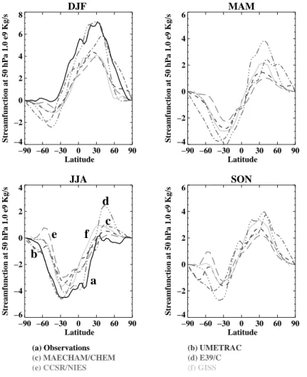
Figure 7 shows the mass streamfunction F_m = 2πaΨ/g at 50 hPa as a function

15

of latitude for the participating models, computed by integrating the second equation downwards withΨ = 0 at p = 0. The observations in the figure are based on ERA-15 for the period 1979 to 1993 (Gibson et al., 1997). The spatial resolution of the original fields was T106 with 31 vertical hybrid levels, equivalent to a grid resolution of 1.125◦or about 125 km. The temporal resolution is 6 h. Note that the ERA data were computed

20

using a GCM with an upper boundary at 10 hPa which may be a limiting factor in representing real variability at 30 hPa and above. The ERA mass streamfunction is a climatological mean over the 15 analysis years.

ACPD

Full Screen / Esc

Print Version Interactive Discussion

c

EGS 2002

For the solstice periods, all the models have the same qualitative shape as the ob-servations with a peak in absolute values occurring in the subtropics of the winter hemisphere. In the northern winter, the results of E39/C agree well with observa-tions between 0◦ and 45◦N but farther north the streamfunction reduces significantly, implying less downward transport. The MAECHAM/CHEM results agree better with

5

observations in high northern latitudes, but there is no indication that this is a result of the higher boundary since the other models are more consistent with the values of the E39/C model in this regard. In the extra-tropics of the northern summer, the E39/C re-sults are higher than observations and the other models, implying too much transport. Most models have the same problem, but to a varying extent in the southern summer.

10

As in the northern winter, the streamfunctions of most models are smaller then ob-served in the southern winter, again indicating insufficient transport. Once more, the impact of the position of the upper boundary appears to be a secondary factor. During the equinox periods, the models are broadly consistent with each other. The E39/C model has slightly higher values of the streamfunction in mid-latitudes than other

mod-15

els, but this may be related to an extended winter regime in the model rather than direct effects of the upper boundary.

For the results presented here, it therefore appears that the impact of the upper boundary position for low top models is smaller than the impact of for example non-orographic gwd in models which simulate the whole stratosphere. It therefore might be

20

concluded that total ozone in the current atmosphere can be reasonably simulated by low top models. However, low top models need higher dissipation immediately below their top than the equivalent higher top models, and this additional dissipation may lead to a reduced response to climate change. Further, low top models are unable to accommodate non-orographic gwd schemes and partly artificial constructs, such as a

25

nucleation barrier for PSC formation, need to be included to compensate for the cold bias.

ACPD

Full Screen / Esc

Print Version Interactive Discussion

c

EGS 2002

3.4. Future predictions of planetary waves and heat fluxes

In some GCMs, there is a significant trend in planetary wave propagation with time. In the GISS GCM, planetary waves are refracted equatorward as greenhouse gases increase (Shindell et al., 2001) while in the ULAQ model there is a marked reduction in the propagation of planetary waves 1 and 2 to high northern latitudes in the doubled

5

CO₂ climate simulated by Pitari et al. (2002). The latest results of the ULAQ model are different to the earlier results based on a much simpler model. It is probable that the model results are sensitive to the changes in static stability in the middle and lower troposphere with an increase in stability from increases in WMGHGs giving rise to an Arctic vortex that is less vulnerable to stratospheric warmings. In the GISS model the

10

impact of changed planetary wave drag is largest during winter when the polar night jet is enhanced (Shindell et al., 1998a; Rind et al., 1998). Planetary wave refraction is governed by wind shear, among other factors, so that enhanced wave refraction occurs as the waves coming up from the surface approach the area of increased wind. They are refracted by the increased vertical shear below the altitude of the maximum

15

wind increase. Equatorward refraction of planetary waves at the lower edge of the wind anomaly leads to wave divergence and hence an acceleration of the zonal wind in that region. Over time, the wind anomaly itself thus propagates downward within the stratosphere (cf. Baldwin and Dunkerton, 2001) and subsequently, from the tropopause to the surface in this model.

20

At high latitudes in the lower stratosphere the direct radiative cooling by greenhouse gases and less radiative heating by ozone due to chemical depletion causes an in-crease in the strength of the polar vortex. Planetary wave changes may be a feedback which strengthens this effect. One proposed planetary wave feedback mechanism (Shindell, 2001) works as follows: tropical and subtropical SSTs increase, leading to

25

a warmer tropical and subtropical upper troposphere via moist convective processes. This results in an increased latitudinal temperature gradient at around 100–200 hPa, leading to enhanced lower stratospheric westerly winds, which refract upward

propa-ACPD

Full Screen / Esc

Print Version Interactive Discussion

c

EGS 2002

gating tropospheric planetary waves equatorward. This results in a strengthened polar vortex.

Other model simulations show qualitatively similar effects on planetary wave prop-agation (Kodera et al., 1996; Perlwitz et al., 2000). Also, the E39/C results (Schnadt et al., 2002) show a small decrease in planetary wave activity for the period 1960 to

5

1990. However, results for future simulations differ depending on the model. Without chemical feedback, the UM (N. Gillett, personal communication, 2001) predicts a fu-ture increase in overall generation of planetary waves, which leads to a greater wave flux to the Arctic stratosphere, and is even able to overcome the radiatively induced increase in the westerly zonal wind so that the overall trend is to weaker westerly flow.

10

This also occurs in E39/C with chemical feedback (Schnadt et al., 2002). Thus E39/C planetary wave activity follows that of the ozone change with decreases in the past and an increase into the future. In the UM with chemical feedback (UMETRAC) the high latitude heat flux (a measure of the wave activity) is apparently downward throughout the period 1975–2020 (Fig. 8), giving a trend of −2.2 ± 3.7%/decade(2σ), which is not

15

statistically significant. The CCSR/NIES model, of lower resolution than UMETRAC, has systematically lower heat fluxes and also shows a downward trend during the pe-riod 1986–2050 of −3.0 ± 3.0%/decade, which is marginally statistically significant. For the shorter period 1986–2001, the trend is much larger (−6.7 ± 13.5%/decade), but the short model record reduces the statistical significance. In the timeslice experiments

20

CMAM and MAECHAM/CHEM show a decrease in high latitude heat flux throughout the periods 1980–2045 and 1960–1990 of 1.0 ± 2.1%/decade and 1.2 ± 3.4%/decade (2σ), respectively, but this is not statistically significant for either model. In general, the degree of strengthening of the polar vortex is critically dependent upon the model used and whether coupled chemistry is incorporated.

25

Observations suggest that in the past twenty years the Arctic vortex has strength-ened (Tanaka et al., 1996; Zurek et al., 1996; Waugh et al., 1999; Hood et al., 1999). Likewise, a trend toward equatorward wave fluxes has also occurred in observations (Kodera and Koide, 1997; Kuroda and Kodera, 1999; Ohhashi and Yamazaki, 1999;

ACPD

Full Screen / Esc

Print Version Interactive Discussion

c

EGS 2002

Baldwin and Dunkerton, 1999; Hartmann et al., 2000) and the total amount of wave activity entering the stratosphere has decreased over the past 20 years (Newman and Nash, 2000; Randel et al., 2002). The trend in the heat flux for the period 1979–2001, shown in Fig. 8 is −6.8 ± 6.7%/decade, just statistically significant but somewhat larger than all the model results presented here. However, in view of the large error bars

5

extrapolation of those trends to the future must remain uncertain. 3.5. Uncertainties in the H₂O rate of increase

Global satellite observations of the middle and upper stratosphere, for the period 1991– 1997, supported by coincident ground-based data (Nedoluha et al., 1998; Randel et al., 1999), and lower stratospheric measurements over Boulder, Colorado and

Washing-10

ton, D. C., covering a longer period 1964–2000 (Oltmans and Hofmann, 1995; Oltmans et al., 2000) all show very large increases of water vapour, in the range of 8–20% per decade. Based on ten datasets incorporating satellite, balloon, aircraft, and ground-based measurements over the period 1954–2000, Rosenlof et al. (2001) reported an overall increase of 1% yr−1in stratospheric water vapour concentrations. Some aircraft

15

observations, however, give conflicting indications of trends in the lower stratosphere (Peter, 1998; Hurst et al., 1999). The evidence largely supports a significant trend in the past, suggesting that a similar trend may take place over the coming decades.

The calculated enhanced rate of water vapour production due to methane increases is sufficient to account for less than half the observed water vapour increase. It is

there-20

fore suspected that there has been increased transport from the troposphere to the stratosphere. This is governed largely by tropical tropopause temperatures (e.g. Mote et al., 1996), and could be greatly altered by changes as small as a few tenths of a de-gree (Evans et al., 1998). Observations do not indicate an overall warming trend at the tropical tropopause (Simmons et al., 1999). However, water vapour fluxes as a function

25

of season and geographic location have not been precisely quantified (SPARC, 2000), so that it is difficult to determine the reason for any increased flux to the stratosphere. For example, a very small shift away from the equator could raise the minimum

tem-ACPD

Full Screen / Esc

Print Version Interactive Discussion

c

EGS 2002

peratures encountered sufficiently to allow a significantly greater upward flux. Thus, an increase in tropospheric water vapour, predicted by most climate models, could lead to increased stratospheric water even without a warmer tropopause. Hartmann et al. (2001) have described a possible mechanism whereby lowering tropopause temper-atures can lead to increased flux of water into the stratosphere. This results from the

5

increased formation and transport of ice particles into the lower stratosphere. Whether any of these or further unidentified processes are responsible for the observed water vapour increase needs further investigation.

Increased water vapour affects ozone chemistry indirectly by decreasing local tem-peratures via radiative cooling, which slows down the reaction rates of ozone depletion

10

chemistry. Increased water vapour also generates OH radicals which chemically de-plete ozone. The effects on homogeneous chemistry have been studied in 2- and 3-D models by Evans et al. (1998), Dvortsov and Solomon (2001), and Shindell (2001). The models all show that the net effect of an increase in water vapour is to reduce ozone in the upper and lower stratosphere, and to increase ozone in the middle stratosphere.

15

The model results differ most in the lower stratosphere where the largest impact on the total ozone column occurs. In the model of Evans et al. (1998), lower stratospheric ozone is reduced only in the tropics when water vapour increases, while in the models, ozone reductions extend to mid-latitudes or to the poles. Thus the models of Dvortsov and Solomon (2001) and Shindell (2001) predict a delay by about 10–20 years in ozone

20

recovery. During the next 50 years, ozone is expected to decrease by 1–2% due to the water vapour increase.

Water vapour increases also affect heterogeneous chemistry, enhancing the forma-tion of PSCs. Kirk-Davidoff et al. (1999) calculated a significant enhancement in Arctic ozone loss in a more humid atmosphere. Much of this effect was based on a very large

25

estimate of 6 to 9 K cooling per ppmv of water vapour increase (Forster and Shine, 1999). However, recent modelling suggests that the true value may be much smaller, about 1.5 to 2.5 K cooling per ppmv of water vapour increase (Oinas et al., 2001). This would in turn imply a reduced overall role for water vapour in enhancing PSC formation.