First-Order Based Non-Linear Open-Loop Identification of a Ionic Polymer Bending Actuator and Derived Linear PI closed-loop Control

HAL Id: hal-02004975

https://hal.archives-ouvertes.fr/hal-02004975

Submitted on 3 Feb 2019

HAL is a multi-disciplinary open access archive for the deposit and dissemination of sci-entific research documents, whether they are pub-lished or not. The documents may come from teaching and research institutions in France or abroad, or from public or private research centers.

L’archive ouverte pluridisciplinaire HAL, est destinée au dépôt et à la diffusion de documents scientifiques de niveau recherche, publiés ou non, émanant des établissements d’enseignement et de recherche français ou étrangers, des laboratoires publics ou privés.

First-Order Based Non-Linear Open-Loop Identification

of a Ionic Polymer Bending Actuator and Derived

Linear PI closed-loop Control

Bertrand Tondu, Aiva Simaite, Philippe Souères, Christian Bergaud

To cite this version:

Bertrand Tondu, Aiva Simaite, Philippe Souères, Christian Bergaud. First-Order Based Non-Linear Open-Loop Identification of a Ionic Polymer Bending Actuator and Derived Linear PI closed-loop Control. CIMTEC 2016, Jun 2016, Perugia, Italy. �hal-02004975�

First-Order Based Non-Linear Open-Loop Identification of a Ionic Polymer

Bending Actuator and Derived Linear PI closed-loop Control

Bertrand Tondu

, Aiva Simaite

, P. Soueres

, C. Bergaud

1

Institut National de Sciences Appliquées, 135 Avenue de Rangueil, 31077 Toulouse, France 2

LAAS, CNRS, 7 avenue du colonel Roche, 31400 Toulouse, France.

Keywords: Artificial muscle, Bending electroactive polymer, Nonlinear identification.

Abstract. Tri-layer electroactive bending polymeric artificial muscles generally exhibit no

overshoot during open-loop step response with a non-zero initial slope when the output is the vertical position of the bending sample tip. If a simple linear first order is not able to capture the variety of step responses when the u-voltage varies along its practical range, we propose to identify such a bending step contraction by a nonlinear system derived from a linear first order system in the form: k(1etr/T)uwhere the parameters k, T and r depend on the u-control voltage. We show the relevance of this approach for identifying the step-response of a PEDOT:PSS/PVDF/ionic liquid actuator developed at the laboratory. As a consequence, we show that a linear PI-controller is a simple and an efficient approach for a closed-loop control of the bending actuator. A simple method taking into account voltage saturation control is proposed and applied to both real steps and sine-wave tracking.

Introduction

Closed-loop control of artificial muscle is a difficult challenge due to the general nonlinear character of the artificial muscle dynamic contraction but also due to its associated feeding requirement. Among possible energy choices, electric tension is particularly relevant as a clean, simple supply mode easy to put into work, especially when a quick contraction can be obtained from low voltage and low electric energy. Ionic polymer bending artificial muscles belong to this class of low energy electroactive polymeric actuators. While, in their earlier development, such bending strips needed a liquid environment for contracting, the recent use of non-evaporable ionic liquid made possible their use in open air [1], [2] and so expanded their application field. Although the positioning of this kind of actuator can be controlled in open-loop with an input voltage, the typical “drift”-phenomenon of the actuator under a constant input voltage – i.e. the fact that the actuator continues to slowly bend without giving the impression to converge towards a steady-state position – makes necessary a closed-loop control. Several attempts have been made for developing closed-loop control for the accurate positioning of this bending artificial muscle including linear PID-control [3], feed-forward control [4], sliding mode control [5] or fuzzy and neuro-fuzzy control [6]. The highly nonlinear character of the bending phenomenon would actually lead to give priority to sophisticated control approaches as done by Druitt and Alici in their most recent paper [6]. In some alternative way, we would like to analyze, in this paper, the relevance to come back to simpler control approaches. Our actual work was inspired by our work made on the control of robots actuated with the pneumatic McKibben muscle: its highly non-linear character led us, as other authors, to test multiple sophisticated closed-loop control approaches such as sliding mode control, fuzzy control or biomimetic control but, although interesting results were obtained for such or such trajectory, all these approaches actually suffer from a degree of complexity due to the relatively high number of parameters or rules to tune without being sure to keep the same level of performance in a large field of experimental conditions. More recently, we attempted – especially

for the control of a single artificial muscle or a joint made of two antagonist pneumatic McKibben muscles – to consider a simple I-controller taking advantage of the own stiffness and damping of any artificial muscle [7]. If the electroactive polymers considered in this paper contract by bending while the McKibben fluidic muscle contracts along its long axis, it is such a linear closed-loop control approach with a limited number of parameters that we propose to apply to a tri-layer PEDOT:PSS/PVDF/ionic liquid sample [8], in which carbon nanotubes have be included [9], in order to increase its resistance to delamination in the full working range [2V, +2V], as illustrated in Figs. 1.a and 1.b. In a broad sense, the originality of our approach is based on the intuitive idea that the classic PID can be especially adapted to the peculiar nature of any artificial muscle. Such an approach finds its place, according to us, in current thinking about redefinition of PID gains tuning rules as done, for example, by Fruehauf et al. [10] – mentioned in [6]. The choice of a PI control, as proposed in this paper, is motivated by the identified model developed in section 1 before we attempt to apply it for steps and sine-wave trajectories in section 2, by means of the classical experimental set-up shown in Fig. 1.c. The sample tip positioning is measured thanks to a laser with respect to a zero horizontal position, and the feedback control combines a NI-card with the LabView software.

1. Non-linear Identification of the Artificial Muscle

In a recent article [11], we attempted to propose a general definition of any artificial muscle as an open-loop stable system when input is the muscle activation variable and output is one positioning dimension. In the case of a tri-layer bending polymeric sample, the input is an electrical voltage while the output is generally specified as a vertical distance measured at the tip of the sample. The open-loop stable character of the artificial muscle points the way towards open-loop identification, especially from step recording of its positioning dimension in response to various step amplitude. Such an identification problem can be tackled by using various methods as the ANFIS-NARX paradigm, recently applied to IPMC (Ionic Polymer Metal Composite) [12] for getting an advanced non-linear model of the full bending actuator or, in a more conventional way, classical techniques of linear system identification applied to the time variation of the sample. In [4], the authors propose a sixth-order transfer function with a constant gain for identifying their polypyrrole tri-layer actuator. Our approach is a bit different in the sense it is based on a preliminary observation of two characteristics of any open-loop step-response of the type of bending actuator we try to control. Whatever the u-control voltage, no overshot occurs and the slope at the origin is never close to zero. In the framework of linear systems, these two elements are characterizing a first-order system. We show in Fig. 2 the result of the identification of the open-loop real step response by a first-order linear model for +/0.25V, +/0.5V, +/0.75V and +/V steps. For each step, in a very classical meaning, the gain k is simply identified as the ratio between the steady-state position, noted x , _

read in practice at a time of 60s, and the corresponding step amplitude, while the time constant, noted T for distinguishing it from the T-parameter considered further in the case of the non-linear _L

model, is determined as the time corresponding to the reached position(11/e)x_. We observe that though for low positive and negative voltages, this linear identification gives satisfactorily results, the higher the step voltage in absolute value, the more the linear model deviates from the real step response. Let us define the mean deviation between the model and the real step response by:

) ( / )) ( ) ( ( 0 x t x t x t Mean _{t t L L} horizon    – wherex k e t TL u

L  (1  / ) and thorizon is a time horizon

equal to 60s. As can be read in Table 1, if this mean deviation is limited to 3.5 % in a

[V,V]-range, it quickly increases beyond. This is due, according to us, especially to the

“drift”-phenomenon which makes the convergence to the steady-state slower than expected for a linear system.

This is the reason why we propose the following non-linear model directly derived from the expression of a first-linear model, as follows:

u e

k t

x_NL( ) (1 tr/T) (1) where u is the step amplitude, x is the artificial muscle tip position, k is a gain, T a time constant-like parameter and r a positive coefficient lower than 1, without dimension. If r=1, the system behaves like a first-order linear system. We propose to identify the three parameters k, r and T, as follows. On the one hand, as previously, the gain k is identified as the ratio between steady-state position and corresponding control voltage with, however, an increased difficulty to accurately determine the steady-state value when the voltage increases in absolute value. On the other hand, the T and r parameters can be determined, according to the following procedure. In a first step, assuming that the real step response behaves exactly as to the non-linear model of Equ. (1), the T and r-parameters are determined as follows:

- At time  T1/r, x()(11/e)x_. It is then possible, by means of a direct measurement of x() to deduce ,

- Because, for a constant u-value,x(t)(kr/T)tr1etr/Tu, we have, at time ,

e rx

x() _/ 1. It is then possible, by a direct reading of the slope x()to deduce the following expression for r: r x()e/x_.

- We finally deduce:Tr.

In a second step, the obtained parameters can be modified in order to minimize the mean deviation error between the model and the real step response as previously defined for the linear model:

) ( / )) ( ) ( ( 0 x t xt x t Mean _{t t NL NL} horizon  

 until this mean deviation becomes less than some imposed limit. This strategy is however highly dependent on the initial x -steady state estimation. If such an _

estimation is easy to do for absolute lower step voltages, it is less obvious for absolute upper u-step voltages due to the drift-phenomenon, and also due to unpredictable change as this can be observed at time 40s for u=1V and u=2V, on Fig. 3.a. For these reasons, we also played with the



x -parameter for matching the real response with the proposed model. We applied this two-step

strategy to voltage steps from +/ 0.25V to +/2V with a 0.25V increment and looking for a mean error between real response and its model less than 2% on a 60s time horizon. For reaching such a goal, depending on the u-step, estimated k and T parameters after the first step were to be modified in a [1%, 25%] range. We show in Figs 3.a and 3.b the final result of this identification, whose corresponding parameters are given in Table 2. By comparison with what was obtained by means of the first-order linear model, the proposed non-linear model now gives a good matching between the real step response and the model for each u-value and, even for the low ones, the non-linear model also gives better results than the linear one. It is also worthy to note the relative dissymmetry between positive and negative step modeling. This effect is usual for bending actuators and our modelling approach makes possible to take it into account. A linear interpolation between identified parameter values for getting continuous change for k, T and r is proposed in Fig. 3.c. It can be noted that we voluntarily limited the interpolation to the ranges [2V, 0.25V] and [+0.25V, +2V] due to the lack of data at very low voltage steps. We see little problem with this situation due to the fact that control voltage close to zero is rarely used in practice.

1 _{From the same time derivative formula, we also get:x}_(t₀₎_{, for any r}_{0. This initial non-physical value} however appears to be non-problematic in our modelling process as it could be explained by the high slope variation between initial and latter bending during step response.

As this can be viewed in Fig. 3.c, the variation of the r-parameter is monotone and decreasing respectively from 0.25V to 2V and from 0.25V to 2V. The same monotone and decreasing character is also globally obtained for the other two parameters, k and T with a tendency for the three parameters (T, k, r) to become independent on u when its value is close to /+ 2V. This interpolated model will be further used for simulating the considered closed-loop control.

A last question concerns the relevance of such a model for other bending actuators. In a general way, we could claim that our approach is relevant for most bending actuators whose open-loop dynamic step response is performed without overshoot, which seems to be often the case with soft ionic polymers. On the contrary, bending IPMC can exhibit step response with a large overshoot followed by a slow descending convergence towards the steady-state. High order linear identification is then necessary for matching the model with the real step response as reported, for examples in [13] for a bending IPMC strip exhibiting an overshoot of about 300%. If we think that soft ionic polymer actuators are one of the most promising way for bending actuators, the proposed non-linear identification could prove all its worth.

2. PI-closed loop control

2.1. Linear tuning and non-linear effects

It is well known that a first order linear system can be controlled in closed-loop by a PI-controller whose proportional and integral gains can be determined from a direct comparison between the resulting characteristic polynomial and the one of a reference second order system. Let us write the PI-control as follows:   d x x k x x k u t d I d p( ) ( )( ) 0



constant gains. For a linear first order, open-loop system, in the form of the transfer function

km/(1+Tms), where km and Tm are respectively the static gain and the time constant, the characteristic

equation resulting from the PI-controller is given by:

0 )] /( [ )] /( ) 1 [( 1 k_mk_P k_mk_I s T_m k_mk_I s2 (3) whose terms can be identified with those of the classic form:12z_ns(1/_n2)s20, where z is the damping factor and n the undamped pulsation of the corresponding linear second order.

Because it is also well known that response time of a linear second-order system without zero is, for a given z, inversely proportional to n , it is then possible to choose z and a given response time Tr –

for example, the time beyond which the response keeps inside the 0.95/1.05 desired position-range – for deriving the gains kp and kI as follows:

)] ) ( and ] 1 ) ( 2 [ 1 2 2 r m m r n I r m r n m P T k T T k T T T z k k      (4) In the limit-case z=1 – corresponding to the quickest step-response before overshooting – the (nTr)-term is equal to about 5 and we can so compute kp and kI for any given Tr . This approach

has, however, a severe limitation: the presence of a zero in the closed-loop transfer function equal to (kI /kp) whose effect can be an overshoot impacting also the response time. Although this can be

highly questionable, let us try to apply this gain tuning approach to the case of our bending actuator. In order to do that let us consider the very rough linear first-order model whose static gain and time

constant are respectively equal to the means of static gains and time constants identified with a simple first-order model. Because in further reported experiments we voluntarily limited us to positive desired positions, we extended the results reported in section 1 to positive u-steps from 0.25V to 2V with a 0.25V-increment and we respectively chose for km and Tm the mean values of

the identified linear first-order static gains and time constants. We got: k_m2.1mm/Vand s 4 . 5  m

T . Choosing z=1 and Tr =2s, the kP and kI parameters can be then directly determined from

Equ. (4). We got:k_P15V/mmandk_I 18V/mm.s. We show on Fig.4 the simulation of this PI-closed loop control applied to the non-linear first-order model developed in section 1 including the model parameter interpolation considered in Fig. 2.c. The obtained result for desired +0.5, +1, +2 and +3mm steps is surprisingly very satisfying: no or a very limited overshoot is got and response time, as previously defined, varies from about 0.7 to 2 seconds. However, as this can be clearly seen in Fig. 4.b, some initial control peak occurs which is, in fact, proportional to the step value. As a consequence, this way of tuning the controller gains is not satisfying as it does not allow to take into consideration the strong constraint peculiar to the considered artificial muscle: control voltage should stay inside imposed limits.

2.2. Taking into account voltage constraints

Theoretically, closed-loop control should avoid reaching the bounds of the admissible control range. But, in the case of our tri-layer sample, the consequence would be the need to adapt the controller gains – or rules if a logics-based controller is considered – to the desired position. The consequence can be a great complexity as already mentioned in the case of the recent study by Druitt and Alici [6]. Our alternative approach proposes to consider the [2V, +2V] voltage range as a practical range whose 2V/+2V bounds can be reached without damage for the artificial muscle at the condition that the steady-state position does not require to indefinitely stay at one of these bounds. According to the open-loop identification developed in section 1, this condition is satisfied by limiting the desired position in the range [3mm, +3mm].

If we admit that closed-loop control can be performed with saturation periods, it is clear that classical rules for tuning a PID-type controller cannot be applied anymore. Our approach for tuning the PI-gains is based on the fact that, on the one hand, only two gains are considered and, on the other hand, on the knowledge of the identified non-linear model. In the case of steps, the following two-stage strategy is proposed, where ulim designates the maximum value for a safe control:

1. A reference xref-position is chosen, typically at the middle of the positive, or negative,

admissible range. The gain kP is then tuned according to the following relationship:

ref

P u x

k  _lim/ (5) Such a kP-gain leads to a control value equal to ulim at t=0+ just before the integral action

starts playing its role;

2. For the same reference position, the gain kI is then tuned by simulation of the PI closed-loop

controller applied to the non-linear model proposed in section 1 with, as an aim, a limited overshoot combined to the lowest possible response time. The obtained (kP , kI) couple can

then be applied to lower and upper desired positions.

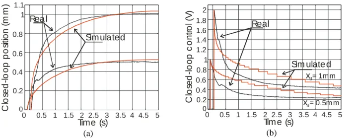
Let us consider, in our case, a reference position equal to 1mm and ulim =+2V. We deduce: kP=2V/mm. As shown in Fig. 5.a, a choice of kI=1 V/mm.s leads to a response time of about 2s with

no overshoot. As expected, the control voltage is saturated at t=0+ and then tends to a non-saturated value, as illustrated in Fig. 5.b. On the same plots, we considered the simulated step-response for

xd=0.5mm: no overshoot occurs and response time is still close to 2s. For each simulated step

response, the corresponding real response and control are represented in Fig. 5.a and 5.b respectively: although the simulated and real curves are close to each other, some discrepancy

appears. This is mainly due to the way the non-linear differential equation has been solved: we used Matlab software and, despite all our efforts, the best solver we could find generated a solution with a mean sampling time of about 300ms when the Labview control program was sampled at 10ms.

Table 3 shows the performances in response time and overshoot for steps between 3mm and +3mm whose corresponding position and control versus time are respectively shown in Figs. 6.a and 6.b. In every step-case, the same (kP , kI)-couple equal to (1V/mm, 2V/mm.s) was used. It can

be checked that, for any desired position greater, in absolute value, than 1mm, the control is initially saturated to +2 or 2 volts before almost instantaneously leaving this value limit. In the case of bounds +3/mm, the control value is initially maintained to the voltage limit during several seconds. This limitation of our actual electroactive artificial muscle makes impossible to get short time responses for desired positions in the lower and upper-range between 3 and 2 mm and +2 and +3 mm. It is worthy to note that for steps lower than 1 mm, in absolute value, another tuning of the gains would make possible to get a faster contraction but our first aim in the reported experiments was to analyze the possibility of keeping the same gains whatever the step-value and, especially, to check the very limited overshoot resulting from such an approach, as verified in Table 3. We also give in Fig. 6.c the steady-state error for positive steps 0.5, 1, 2 and 3mm: in every case, the steady-state error belongs to the [0.02mm, +0.02mm]-range which exhibits the very positive role of the integral action.

2.3. Stability of the PI-controller

A linear first-order system with a PI-feedback control is always stable whatever the choice of the positive kP and kI gains because its characteristic polynomial is a second-order one with positive

coefficients. At the opposite, the same first order system with a three-term PID-feedback control is unstable for a kI-gain whose value limit is given by the Runge-Kutta criterion. What happens in the

case of our non-linear artificial muscle model? Let us assume that the artificial muscle has been put in the equilibrium position xequ by means of a control voltage equal to uequ which must verify the

steady-state relationship: xequ=kuequ. Let us assume that we move the system from this equilibrium

position, briefly and within a short distance, in order that we can assume that the parameters k, r and

T keep constant. As a consequence, the PI generates a closed-loop control voltage given by Equ.

(2) where xequ has to be written instead of xd. By deriving Equ. (1), we get:

    _{ } k e u rT t  e u x (1 tr/T)( / )1 r) tr/T (6) By putting into Equ. (6) the expression of uresulting from the time derivative of the control equation imposed by the PI as follows: uk_Pxk_I(x_equx) , the following differential equation of the closed-loop system results:

u e t T kr e x x kk e kk x[1 _P(1 tr/T)] _I( _equ )(1 tr/T)( / ) r1 tr/T (7) where k, r, and T depend on u according to the relationship identified in section 1. When t tends to infinite, due to the fact that, for0r1, etr/Tand tr1etr/Ttend to zero, Equ. (7) is reduced to:

) ( ) 1 ( kk kk x x x _P  _{I equ} (8) This last equation is similar to the one resulting from the closed-loop control by a PI of a first-order linear system in the form: xk(1et/T)u. We can so conclude from the accurate knowledge of the proposed actuator model that the considered PI-controller stabilizes the closed-loop system. A very

interesting practical consequence is that any blind tuning of the two considered gains cannot put the closed-loop system into instability, whereas a blind tuning of the three gains of a PID could do it.

2.4. Tracking performances

The method for tuning the (kP, kI)-gains proposed in section 2.2 is not applicable to the choice of a

trajectory to be tracked due to the fact that the kP-gain cannot be derived from a simple saturation

constraint as expressed in Equ. (5). An alternative way for tuning the two gains can however be deduced in this case from the fact that, in steady-state, the considered actuator model behaves like a first order whose only gain k and time constant T are depend on control u. We can indeed write the following equivalence in the neighborhood of infinite time, for 0r1and whatever T :

      t e e tr T tT ) 1 ( ) 1 ( / / ₍₉₎

because, when t tends to , (1etr/T)/(1et/T)tends to 1. As a consequence, and considering mean constant values for k and T, we can deduce, from classical results on tracking errors of first linear order systems in closed-loop with a PI, the following estimation of the tracking error V in

response to a constant slope:

) /( _{mean I}

VV k k

 (11) where V is the value of the slope, kmean is the mean value for k, either in positive or negative u-range

and kI is the already defined integral gain. Fig. 7 shows tracking results obtained for various

sine-waves. For the tracking of a sine-wave of +/2mm, with a period of 20s, a nearly constant tracking error can be observed in a large portion between sine-wave extrema, as shown in Fig. 7f and on the close-up view of the first ¾ period of Fig. 8.a: from time about 8s to 12s, the tracking error (x_dx) varies, in absolute value, between about 0.06mm and 0.08mm. By estimating the corresponding slope, in absolute value, to about 0.6mm/s and considering a mean value kmean roughly equal to

2.1mm/V, and because a kI=5 was considered in the reported experiment, from Equ. (11), V can

then be estimated, in absolute value, to about 0.57mm, which is in relative good accordance with the reported experimental values. This emphasizes the relevance of our approach. Another fact is also a direct consequence of the interpretation of the simple dynamic behavior as a first order system and its PI-control in steady-state: the deviation of the real trajectory from the desired one when the curvature is increasing or decreasing. Indeed it is well known that, in the case of a first-order system with PI-closed loop, for input time-signals in the form tr, r>1, the tracking error tends to be infinite with, as a consequence, a maximum tracking error occurring just after each sine-wave extremum as this can be verified in Figs 7.b and 7.d.

We can now better understand the respective roles of kP and kI of our PI-control applied to our

bending actuator in trajectory tracking: kI is the sole gain responsible for the tracking error, when kP

is an additional gain for controlling the transitory state. From the conclusion of section 2.3, there is no risk of instability to increase kI to get a better tracking error for constant slope as to limit

deviation between desired trajectory and real one during non-straight line parts, expect that we are limited by the imposed control range [ulim, +ulim]. We show in Fig. 6.e, and on the close-up view

of Fig. 8.a, the effect of a control saturation imposed, in our case, to +/2V. As shown on Fig. 8.b, the control is saturated just before the system reaches the top of the sine-wave: as a consequence, the system behaves as an open-loop system and cannot continue to efficiently track the sine-wave. Contrary to case without saturation, the real trajectory is now below the desired one and the shape of the sine-wave is no more preserved.

From all these remarks and because we wanted in this paper to analyze the possibility of a PI-controller with same constant gains for a set of desired trajectories, we considered the following strategy applied to a family of given sine-waves:

- Because kP is essentially devoted to transitory state dynamics, its value is chosen to be equal

to the one determined in step gain tuning,

- Considering a sine-wave of the maximum desired amplitude, kI is chosen such that +/ulim is

reached at sine-wave top/bottom.

We applied this strategy for tracking sine-wave with amplitude between +/0.5mm and +/2mm. Three examples are reported for which amplitudes and associated time period were chosen as follows: +/0.5mm with a time period of 5s, +/1mm with a time period of 10s and +/2mm with a time period of 20s. Keeping kP equal to 2, a kI equal to 5 was practically chosen from the

observation of a control saturated respectively to +2V and 2V when the sine-wave of +/2mm reaches respectively the neighborhood of its maximum and minimum. From the reading of Figs. 7.b, 7.d, 7.f, it can be seen that the tracking errors are respectively in the ranges [2mm, +0.2mm], [mm, +0.15mm] and [m, +0.3mm] for the three considered examples. It is interesting to remark that the error obtained in the third example (amplitude of +/2 mm at a 0.05 Hz frequency) is not so far from the result reported by Yao, Alici and Spinks [3] with a much faster tri-layer bending actuator (see especially the figure 6 of the mentioned paper).

Conclusion and future work

The proposed PI-controller for closed-loop position control of bending actuators was motivated by an original identification of the actuator under the form of a kind of non-linear first-order system as follows x(t)k(1etr/T)u, where the three parameters k, r and T vary with the u-control voltage.

This simple non-linear identified model leads us to justify the relevance of a simple PI-controller for an efficient and stable closed-loop control of the actuator. In the case of a step-response, a simple tuning methodology for the two gains was proposed: it is based on the specification of a safe control voltage range [ulim, +ulim] and on the possibility given to the control to reach such safe

working limits. Given a reference position xref, belonging to the admissible position range derived

from the specification of the control voltage-range, the kp-gain is given by the simple relationship:

ref

P u x

k  _lim/ ; the kI-gain can then be tuned in order to get the best compromise between no

overshoot and quickest response time. As reported, a fine tuning for kI can be obtained by

simulating the PI-controller with the proposed non-linear bending artificial muscle model. Reported results show the relevance of this approach for getting a same couple of gains in the full position range leading to a maximum overshoot of 5% and a response time taking advantage of the imposed safe voltage limits. The PI-controller is also applied to sine-wave trajectory tracking. In this case, we tried to highlight the analogous behaviour of the studied artificial muscle with a linear first-order system when steady state is established and, as a consequence, the fundamental role of the kI-gain

for limiting the tracking error. Such a similarity also emphasizes the limitation of our PI-control when sharp trajectory curvature changes occur. Future work will focus on improvements in trajectory tracking, especially, by studying the relevance of variable P and I-gains to tackle both sharp curvature changes and voltage saturation constraints.

References

[1] W. Lu, A.G. Fadeev, B. Qi, E. Smela, B.R. Mattes, J. Ding, G.M. Spinks, J. Mazurkiewiez, D. Zhou, G. Wallace, D.R. MacFarlane, S.A. Forsyth, M. Forsyth, Use of Ionic Liquids for  -conjugated Polymer Electrochemical Devices, Science. 297 (9 août 2002) 983-987.

[2] M.D. Bennett, D.J. Leo, Ionic Liquids as Stable Solvents for Ionic Polymer Transducers, Sensors & Actuators A. 115 (2004) 79-90.

[3] Q. Yao, G. Alici and G.M. Spinks, Feedback Control of Tri-Layer Polymer Actuators to Improve their Positioning Ability and Speed of Response, Sensors and Actuators, A, 144 (2008), 176-184.

[4] S.W. John, G. Alici and C.D. Cook, Inversion-based Feedforward Control of Polypyrrole Trilayer Bender Actuators, IEEE/ASME Transactions on Mechatronics. 15(1) (2010) 149-156. [5] X. Wang, G. Alici and C.H. Nguyen, Adaptive Sliding Mode Control of Tri-Layer Conjugated Polymer Actuators, Smart Material Structures. 22 (2013) 1-8.

[6] C. M. Druitt, Intelligent Control of Electroactive Polymer Actuators Based on Fuzzy and Neurofuzzy Methodologies, IEEE/ASME Transactions on Mechatronics. 19(6) (2014) 1951-1962. [7] B. Tondu, What is an Articial Muscle? A Systemic Approach, Actuators. 4(4) (2016) 336-352. [8] A. Simaite, B. Tondu, P. Soueres and C. Bergaud, Hybrid PVDF/PVDF-graft-PEGMA Membranes for Improved Interface Strength and Lifetime of PEDOT:PSS/PVDF/Ionic Liquid Actuators, ACS Applied Materials & Interfaces, 7(36) (2015) 19966-19977.

[9] A. Simaite, F. Mesnilgrente, B. Tondu, P. Soueres and C. Bergaud, Towards Inkjet Printable Conducting Polymer Artificial muscle, Sensors & Actuators B: Chemical, 229 (2016) 425-433. [10] P.S. Fruehauf, I.L. Chien and M.D. Laurister, Simplified IMC-PID Tuning Rules. ISA Transactions, 33 (1994) 43-59.

[11] B. Tondu, Robust and Accurate Closed-Loop Control of McKibben Artificial Muscle Contraction with a Single Integral Action, Actuators. 3(2) (2015) 142-165.

[12] M. Annabestani and N. Naghavi, Non Linear Identification of IPMC Actuators based on ANFIS-NARX Paradigm, Sensors & Actuators A. 209 (2014) 140-148.

[13] N.D. Bhat and W.-J. Kim, Precision Position Control of Ionic Polymer Metal Composite, Proc. of the 2004 American Control Conference, Boston (2004) 740-745.

(a) (b)

(b)

Figure 1: Structure of the tri-layer actuator considered in this study (a) under the form of a sample of 15 mm long, 2 mm wide with a thickness of about 140 m (b) and classical set-up for a closed-loop control of the actuator tip position x towards a desired position or time-trajectory xd (c).

Labview

software

NI card

x

Bending actua tor

Laser

+

_x

x

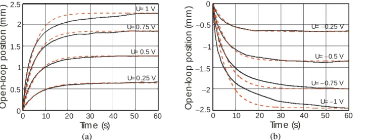
(a) (b)

Figure 2: Attempt to identify the bending actuator as a linear first-order system for +/0.25V, +/0.5V , +/0.75V and +/V steps, (a) Positive steps, (b) Negative steps – real step response is drawn in full line while model is drawn in dashed line.

0 10 20 30 40 50 60 0 0.5 1 1.5 2 2.5 Tim e (s) 0 10 20 30 40 50 60 0 0.5 1.5 2 2.5 U= 0.25 V U= 0.5 V U= 0.75 V U= 1 V O p e n -l o o p p o si ti o n ( m m ) 1 0 10 20 30 40 50 60 -2.5 -2 -1.5 -1 -0.5 0 Tim e (s) 0 10 20 30 40 50 60 0 0.5 U= 0.25 V U= 0.5 V U= 0.75 V U= 1 V O p e n -lo o p p o si ti o n ( m m ) 1 1.5 2 2.5

(a) _(b)

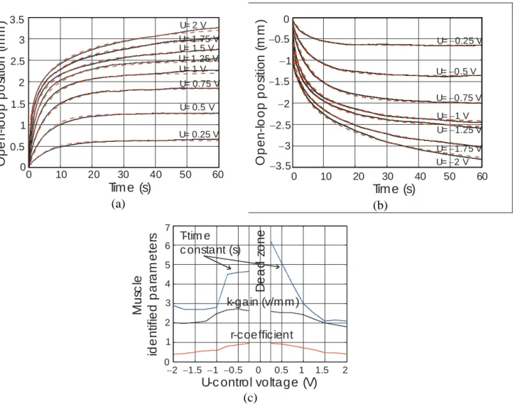
(c)

Figure 3: Nonlinear open-loop identification of the actuator: (a), (b) Comparison between x-position in response to u-voltage steps (full line) and the proposed non-linear model (dashed line), (c) Variation of the parameters (T, k, r) of the proposed nonlinear first-order model foru-control voltage varying in the ranges [2V,0.25V] and [+25V,+2V].

0 10 20 30 40 50 60 0 0.5 1 1.5 2 2.5 3 3.5 Tim e (s) 0 10 20 30 40 50 60 0 0.5 1 1.5 2 2.5 3 3.5 U= 0.25 V U= 0.5 V U= 0.75 V U= 1 V U= 1.5 V U= 1.75 V U= 2 V U= 1.25 V O p e n -l o o p p o si ti o n ( m m ) 0 10 20 30 40 50 60 -3.5 -3 -2.5 -2 -1.5 -1 -0.5 0 Time (s) 0 10 20 30 40 50 60 0 0.5 1 1.5 2 2.5 3 3.5 U= 0.25 V U= 0.5 V U= 0.75 V U= 1 V U= 1.75 V U= 2 V U= 1.25 V O p e n-lo o p p o si ti on (m m ) -2 -1.5 -1 -0.5 0 0.5 1 1.5 2 0 1 2 3 4 5 6 7

U-c ontrol voltage (V)  2 1.5 1 0.5 0 0.5 1 1.5 2  0 1 2 3 6 4 5 r-coe fficient k-ga in (v/m m ) T-tim e c onstant (s) M u sc le id e n tif ie d p a ra m e te rs D e a d z o n e 7

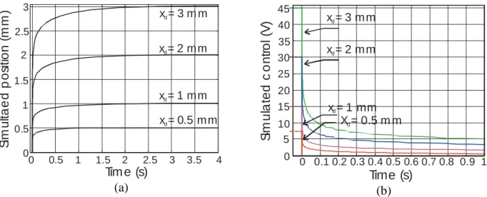
(a) _(b)

Figure 4. Simulation of a closed-loop PI-linear control applied to the actuator non-linear model (see text for gain tuning): (a) Step response, (b) Corresponding control voltage (initial control value is indicated by a short dotted line).

0 0.5 1 1.5 2 2.5 3 3.5 4 0 0.5 1 1.5 2 2.5 3 Tim e (s) 0 0.5 1 1.5 2 2.5 3 3.5 40 2 1 Si m u lta e d p o si tio n ( m m ) 0.5 2.5 1.5 3 x = 0.5 m md x = 1 mmd x = 2 mmd x = 3 m md 0 0.1 0.2 0.3 0.4 0.5 0.6 0.7 0.8 0.9 1 0 5 10 15 20 25 30 35 40 45 Time (s) 0 0.1 0.2 0.3 0.4 0.5 0.6 0.7 0.8 0.9 1 0 20 10 Si m u la te d c o n tr o l ( V ) 5 35 x = 3 m md 15 25 30 40 45 x = 2 m md x = 1 mmd X = 0.5 m md

(a) (b)

Figure 5. Simulation of a closed-loop PI-linear control, including voltage constraints, applied to the actuator non-linear model and comparison with the real closed-loop step response: (a) Step response, (b) Corresponding control voltage.

20 20.5 21 21.5 22 22.5 23 23.5 24 24.5 25 0 0.2 0.4 0.6 0.8 1 Time (s) 0 0.5 1 1.5 2 2.5 3 3.5 4 4.5 50 0.8 0.4 C lo se d -l o o p p o si tio n ( m m ) 0.2 1 Rea l 0.6 1.1 Sim ulated 20 20.5 21 21.5 22 22.5 23 23.5 24 24.5 25 0 0.2 0.4 0.6 0.8 1 1.2 1.4 1.6 1.8 2 Tim e (s) 0 0.5 1 1.5 2 2.5 3 3.5 4 4.5 50 0.8 0.4 C lo se d -l o o p c o n tr o l ( V ) 0.2 1 Real 0.6 1.2 Sim ulate d 1.4 1.6 1.8 2 xd= 0.5m m xd= 1mm

(a) (b)

(c)

Figure 6. Closed-loop positioning of the bending actuator by means of a linear PI control with the same constant (kP,kI)-gains: (a) Step response in the range [3mm, +3mm], (b) Corresponding

control in the case of positive desired positions, (c) Corresponding variation of the steady-state error in the case of positive desired positions between time 60s and time 100s.

20 25 30 35 40 45 50 55 60 65 70 -3 -2 -1 0 1 2 3 Tim e (s) 20 25 30 35 40 45 50 55 60 65 70 0 2 3 1 C lo se d -l o o p p o si tio n ( m m ) 1 2 3 20 30 40 50 60 70 80 90 100 0 0.2 0.4 0.6 0.8 1 1.2 1.4 1.6 1.8 2 Tim e (s) 20 25 30 35 40 45 50 55 60 65 70 0 1.8 2 1 C o n tr o l v a lu e ( V ) _1.6 1.4 1.2 0.8 0.6 0.4 0.2 x = 3mmd x = 2m md x = 1m md x = 0.5m md 60 65 70 75 80 85 90 95 100 -0.02 -0.015 -0.01 -0.005 0 0.005 0.01 0.015 0.02 Tim e (s) 60 65 70 75 80 85 90 95 100 0 0.015 0.02 St e a d y s ta te e rr o r ( m m ) 0.01 0.005 x = 3m md x = 2m md x = 1m md x = 0.5mmd 0.005 0.010 0.015 0.02

(a) _(b)

(c)

(d)

(e) (f)

Figure 7. Tracking of a sine-wave trajectory by means of a PI closed-loop control with constant gains (kP=2, kI=5): (a), (b) Case of a [5mm, +0.5mm]-range sine-wave with a time period of 5 s

and corresponding tracking error, (c), (d) Case of a [1mm, +1mm]-range sine-wave with a time period of 10 s and corresponding tracking error, (e), (f) Case of a [2mm, +2mm]-range sine-wave with a time period of 20 s and corresponding tracking error.

0 10 20 30 40 50 60 -0.5 -0.4 -0.3 -0.2 -0.1 0 0.1 0.2 0.3 0.4 0.5 Tim e (s) 0 10 20 30 40 50 60 0 0.2 0.4 0.5 0.1 C lo se d -l o o p p o si tio n ( m m ) Desired Rea l 0.3 0.1 0.2 0.3 0.4 0.5 0 10 20 30 40 50 60 -0.2 -0.15 -0.1 -0.05 0 0.05 0.1 0.15 0.2 Tim e (s) 0 10 20 30 40 50 60 0 0.2 0.15 Tr a c ki n g e rr o r ( m m ) 0.10 0.10 0.2 0.15 0.05 0.10 0.05 0 10 20 30 40 50 60 -1 -0.8 -0.6 -0.4 -0.2 0 0.2 0.4 0.6 0.8 1 Time (s) 0 10 20 30 40 50 60 0 0.2 0.4 0.8 1 C lo se d -lo o p p o si ti o n ( m m ) Desired Rea l 0.6 1 0.2 0.8 0.4 0.6 0 10 20 30 40 50 60 -0.15 -0.1 -0.05 0 0.05 0.1 0.15 Tim e (s) 0 10 20 30 40 50 60 0 0.15 Tr a c ki n g e rr o r ( m m ) 0.10 0.15 0.05 0.10 0.05 0 10 20 30 40 50 60 -2 -1.5 -1 -0.5 0 0.5 1 1.5 2 Tim e (s) 0 10 20 30 40 50 60 0 0.5 1.5 2 C lo se d -l o o p p o si tio n ( m m ) Desired Rea l 1 0.5 1 1.5 1.5 2 0 10 20 30 40 50 60 -0.3 -0.2 -0.1 0 0.1 0.2 0.3 Time (s) 0 10 20 30 40 50 60 0 0.3 0.2 0.3 0.1 0.2 0.1 Tr a c ki n g e rr o r ( m m )

(a) (b)

Figure 8. Close-up of the tracking performance (a) and associated control (b) in the case of the +/2mm amplitude sine-wave shown on the first ¾ period equal to 15 s – every gradation in time is equal to 0.5 s (see text).

0 5 10 15 -2 -1.5 -1 -0.5 0 0.5 1 1.5 2 Tim e (s) 0 5 10 15 0 1.0 1.5 C lo se d -l o o p p o si tio n ( m m ) 0.5 2 2.0 _x d x 10(x_dx) 1.5 1.0 0.5 0 5 10 15 -2 -1.5 -1 -0.5 0 0.5 1 1.5 2 Tim e (s) 0 5 10 15 0 1.0 1.5 C o n tr o l v a lu e ( V ) 0.5 2 2.0 1.5 1.0 0.5

Table 1. Static gain (k) and time constant (TL) resulting from the identification of the bending

actuator as a linear first-order system and corresponding mean deviation (see text)

u (V) 1 0.75   0.5 0.25 0.25 0.5 0.75 1 k (mm /V) 2.5 2 .7 2.7 2.6 2.5 2.5 2.4 2.2  TL (s) 5.5 6.2 5.6 5.2 6 .8 5.7 5.2 4.5 Mea n error (%) 8.8 5 .8 3.4 2.5 2.5 2.6 2.9 4.2

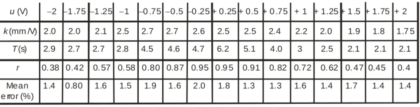
Table 2.Identified parameters of the proposed non-linear model and mean error between the real step response and the proposed model.

u (V) 2 1 .75 1 .25 1 0 .75 0.5 0 .25 + 0.25 + 0.5 + 0 .75 + 1 + 1.25 + 1 .5 + 1.75 + 2       k (mm /V) 2.0 2.0 2.1 2.5 2.7 2.7 2.6 2.5 2.5 2.4 2.2 2.0 1.9 1.8 1.7 5 T (s) 2.9 2.7 2.7 2.8 4.5 4.6 4.7 6.2 5.1 4.0 3 2.5 2.1 2.1 2.1 r 0. 38 0.42 0. 57 0. 58 0.80 0.87 0.95 0.9 5 0.91 0. 82 0.72 0. 62 0. 47 0.45 0. 4 Mean 1.4 0.80 1.6 1.5 1.9 1.6 2.0 1.8 1.3 1.3 1.6 1.4 1.7 1.4 1.4 e rror (%)

Table 3. Estimated response time and overshoot for desired steps in the range [3mm, +3mm] 

x