Root cause analysis of actuator fault based on invertibility of interconnected system

(1)

HAL Id: hal-01763870

https://hal.archives-ouvertes.fr/hal-01763870

Submitted on 11 Apr 2018

HAL is a multi-disciplinary open access archive for the deposit and dissemination of sci-entific research documents, whether they are pub-lished or not. The documents may come from teaching and research institutions in France or abroad, or from public or private research centers.

L’archive ouverte pluridisciplinaire HAL, est destinée au dépôt et à la diffusion de documents scientifiques de niveau recherche, publiés ou non, émanant des établissements d’enseignement et de recherche français ou étrangers, des laboratoires publics ou privés.

Root cause analysis of actuator fault based on

invertibility of interconnected system

Mei Zhang, Ze-Tao Li, Michel Cabassud, Boutaib Dahhou

To cite this version:

Mei Zhang, Ze-Tao Li, Michel Cabassud, Boutaib Dahhou. Root cause analysis of actuator fault based on invertibility of interconnected system. International Journal of Modelling, Identification and Control, Inderscience, 2017, vol. 27 (n° 4), pp. 256-270. �10.1504/IJMIC.2017.10005535�. �hal-01763870�

(2)

To cite this version :

Zhang, Mei

and Li, Ze-tao and Cabassud, Michel

and Dahhou,

Boutaïeb

Root cause analysis of actuator fault based on invertibility of

interconnected system. (2017) International Journal of Modelling

Identification and Control, vol. 27 (n° 4). pp. 256-270. ISSN 1746-6172

O

pen

A

rchive

T

OULOUSE

A

rchive

O

uverte (

OATAO

)

OATAO is an open access repository that collects the work of some Toulouse researchers

and makes it freely available over the web where possible.

This is an author’s version published in :

http://oatao.univ-toulouse.fr/19824

Official URL :

https://doi.org/10.1504/IJMIC.2017.10005535

Any correspondence concerning this service should be sent to the repository administrator :

tech-oatao@listes-diff.inp-toulouse.fr

(3)

Root cause analysis of actuator fault based on

invertibility of interconnected system

Mei Zhang

Electrical Engineering School, Guizhou University,

550025, Guiyang, China and

CNRS, Laboratoire de Génie Chimique, F-31030 Toulouse, France

and

UPS, Laboratoire de Génie Chimique, Univ de Toulouse,

F-31030 Toulouse, France Email: mei.zhang@ensiacet.fr

Ze-tao Li*

Electrical Engineering School, Guizhou University,

550025, Guiyang, China Email: gzgylzt@163.com *Corresponding author

Michel Cabassud

CNRS, Laboratoire de Génie Chimique, F-31030 Toulouse, France

and

UPS, Laboratoire de Génie Chimique, Univ de Toulouse, F-31030 Toulouse, France Email: michel.cabassud@ensiacet.fr

Boutaïeb Dahhou

CNRS, LAAS, F-31400 Toulouse, France and UPS, LAAS, Univ de Toulouse, F-31400 Toulouse, France Email: boutaib.dahhou@laas.fr

Abstract: This paper addresses the problem of root cause analysis (RCA) of actuator fault. By

considering an actuator as an individual dynamic subsystem connected with process dynamic subsystem in cascade, an interconnected system is then constituted. The fault detection and diagnosis (FDD) algorithm is carried out in actuator subsystem and aims at identifying the root causes of actuator faults. According to real plant, outputs of the actuator subsystem are assumed inaccessible and are reconstructed by measurements of the global system, thus providing a means of monitoring and diagnosis of the plant at both local and global level. A condition of invertibility of the interconnected system is first developed to guarantee that faults occurring in the actuator subsystem will affect the measured output of the global system distinguishably. For that, a necessary and sufficient condition is proposed to ensure invertibility of the interconnected system. Effectiveness of the proposed approach is demonstrated on an intensified HEX reactor.

Keywords: root cause analysis; RCA; interconnected system; invertibility; fault detection and

diagnosis; FDD; actuator FDD; input reconstruction; left invertibility; control valve; actuator subsystem; process subsystem; adaptive observer.

(4)

Reference to this paper should be made as follows: Zhang, M., Li, Z-t., Cabassud, M. and

Dahhou, B. (2017) ‘Root cause analysis of actuator fault based on invertibility of interconnected system’, Int. J. Modelling, Identification and Control, Vol. 27, No. 4, pp.256–270.

Biographical notes: Mei Zhang received her Master’s in Automatic from the Guizhou

University, China in 2006. She is currently a co-supervised PhD student at automation in Université Paul Sabatier of Toulouse, France and Guizhou University, China. Her research interests are on the field of advanced control and diagnosis in real-time of dynamic systems with emphasis on dynamical invertible system.

Ze-tao Li received his Master’s degree at the Guizhou University of Technology, Guiyang, China in 1986. In 2006, he obtained his Doctorate degree in Automation from the INSA, France. He is currently a Professor of Electrical Engineering School of Guizhou University, Guiyang, China. His research interests include modelling, identification, predictive and adaptive control of linear and nonlinear systems. He has published over 25 technical papers and co-author of the book

Identification. He is currently the Dean of Electrical Engineering School of Guizhou University,

Guiyang, China and a member of several Chinese scientific committees.

Michel Cabassud is a Professor at the Université Paul Sabatier of Toulouse, France. He earned his Engineer degree at the ENSIC/INPL Nancy and PhD in Chemical Engineering at the LGC/INP Toulouse. He has 25 years of research experience in reactors dynamic simulation, optimisation and control in the field of fine and pharmaceutical industry and is now focusing on batch to continuous reactors transposition. He is the author of more than 80 published papers and 180 communications, three licenses and five book chapters. He is also the French Academic Representative at the Working Party ‘Process Intensification’ of the European Federation of Chemical Engineering.

Boutaïeb Dahhou received his PhD in Process Computer Control in June 1980. He is a Professor at the Paul Sabatier University in Toulouse and is detached to the L.A.A.S. – C.N.R.S. (Laboratoire d’Analyse et d’Architecture des Systèmes) for his research activities. His research concerned the adaptive control and filtering of industrial process control. His research activity deals with the supervision of the industrial processes and particularly fault detection and isolation and fault tolerant control. He was the Director of the Department of Electrical Engineering and Industrial Computer from 2006 to 2012. He is currently a member of several scientific committees within the Paul Sabatier University. He is the author of over 260 publications in international journals and international conferences. He has trained about 25 PhD degrees.

1 Introduction

Modern control system often consists of large number of interconnected sensors, actuators and system components. Technological advancements have made these units increasingly integrated and complex. Each unit may consist of more than one component connected in any configuration, therefore each unit itself is a dynamic system and exhibits complicate system dynamics. For instance, a valve actuator is an assembly of positioner, pneumatic servo-motor and control valve. A failure of any of these units results in the failure of the entire system. In all situations, a dynamical system or a subsystem can be analysed at different levels down to the component level in estimating the reliability of the whole plant.

In this work, we focus on actuator faults. Many fault detection and diagnosis (FDD) methods are presented in the literature for nonlinear dynamic systems subject to actuator fault. One main category is system level-based diagnosis approach which aims at detecting and identifying fault existence and location from the view point of global system. Another common kind focuses on the field component level which aims at analysing internal dynamics of a specific actuator.

Current FDD methodologies typically focus on system level where the major objective relates to performance supervision of the final product. In these methods, dynamics of field devices (i.e., actuator) is normally ignored, instead, they are treated as a component which is viewed as constant in the input/output coefficient matrix/function of the process system model. A key approach is based on residual generation. In Persis and Isidori (2001), a nonlinear FDI filter is designed for generating residuals using a geometric approach, theses residuals are affected by a particular fault and not affected by disturbances and the rest of faults. Besides, actuator fault isolation is studied by exploiting the system structure to generate dedicated residuals (see Methnani, 2013; Chen et al., 2005; Li and Dahhou, 2006). In this approach, each residual, defined as the differences between state measurements and their expected trajectories, is uniquely sensitive to one fault. Thus, a fault is isolated when the corresponding residual breaches its threshold. In addition, adaptive estimation techniques are used to explicitly account for unstructured modelling uncertainty for a class of Lipschitz nonlinear systems (see Zhang et al., 2010; Fragkoulis et al., 2011; Farza et al., 2007). In these results, residuals, defined as output estimation errors, and time-varying thresholds are generated using a bank of estimators, and a fault is isolated when the corresponding

(5)

residuals breach their thresholds. Another approach different to residual generation is fault estimation or fault reconstruction which can determine the size, location and dynamics behaviour of the fault. The relevant literature on this topic has its roots on system inversion theory (Pinheiro and Araújo, 2013). There are several techniques available for fault reconstruction: sliding mode observers (Xu et al., 2012; Edwards et al., 2012; Martínez-Guerra et al., 2013), unknown input observers (Manaa et al., 2015; Blesa et al., 2014; Nagy-Kiss and Schutz, 2013; Zarei and Shokri, 2014), input reconstruction (Maksimov and Pandolfi, 2001; Yang et al., 2015; Szigeti et al., 2002; Schubert et al., 2012; Edelmayer et al., 2004). The key requirement is to completely decouple the faults from the effect of disturbances and also the input signals.

With respect to the above results, fault symptoms can be detected without having the capability to pinpoint the root causes of these faults. For example, Benaïssa et al. (2008) show that decrease of measured temperature in HEX/reactor may be due to decrease of fluid flowrate, this implies an actuator fault. With the help of above FDD algorithms, we can detect and isolate the actuator fault, but fail to realise the root cause of the fault in that particular actuator. The involving candidate root causes of this fault could be valve clogging, stop of utility fluid pump or leakage. A main reason that leads to this is that actuator is treated as a component, rather than a dynamic system in the process. Varying failure signatures are denoted by the changes of elements of the input matrix function. Therefore, the applications of the above FDD methodologies mainly limit to the existence and the isolation of a fault at a global level, while seldom further efforts are made for root cause analysis (RCA) of the detected fault. However, a single disturbance may indicate more than one candidate of root causes. Hence, the determination of these malfunctions of subcomponents, especially those small and incipient faults, before they become serious has important influences on safety and productivity.

In order to examine potential relationship from causes to effects of an actuator fault, efforts have been made to locate subcomponent faults for RCA from the view point of component level. There are two main kinds: self-validating and FDD method, however, both kinds are restricted to local level. The former one only self-diagnosis from local level as so called smart actuator (Yang and Clarke, 1999). Smart actuator is independent of FDD approach; it is an instrument that is designed to compensate for its own undesirable inherent characteristics, to correct from fault conditions, e.g., smart positioner in Bartyś et al. (2006). Also, there are FDD involved methods by which actuator are treated as a dynamic system. Sarosi et al. (2015) propose an algorithm to detect valve stiction for diagnosis of oscillation. Other artificial neural network-based methods for fault diagnosis can be found in Subbaraj and Kannapiran (2014), Zhang (2011) and McGhee et al. (1997). Model-based FDD approaches are proposed in Wickramatunge and Leephakpreeda (2013), Roy et al. (1998) and Ding and Zhao (2014). For example, Puig et al. (2006) develops an interval

observer-based passive fault detection method for control valve. But these available results are limited to actuator level and fail to monitor the whole process simultaneously. It is because the component level-based diagnosis method focuses only on management of the subsystems that use the local information, i.e., states/outputs of this subsystem. Another challenge when researching FDD methods locally is getting data from the subsystem being observed to develop and validate these methods, because physical measurements of actuators are often not possible or difficult owing to distances or rough environment.

In summary, there is a lack of results on actuator FDD that allows to implement advanced FDD methods capable of RCA at local level, as well as of system supervision at global level. Motivated by the above considerations, the main contribution of this paper is to combine RCA of fault from a local level with generally global system supervision. The objective is to explain how the behaviour of global output can be interpreted to identify root cause of actuator faults in actuator subsystem. We propose a left invertible interconnected nonlinear system structure with input reconstruction laws which is based on dynamic inversion, forming a new model-based actuator FDD and RCA algorithm. Actuator is viewed as subsystem connected with the process subsystem in cascade manner, thus identifying reasons of actuator faults with advancing FDD algorithm in actuator subsystem. Outputs of the actuator subsystem are assumed unmeasured and reconstructed by measured global outputs. The left invertibility of individual subsystem is required for ensuring that faults occurring in actuator subsystem can be transmitted to the process subsystem uniquely, and for reconstructing inputs of process subsystem, also outputs of actuator subsystem, from measured global outputs. The developed fault diagnosis algorithm is an effort to combine the strength of system level and the component level model-based fault diagnosis.

The paper is organised as follows. Section 2 describes the proposed strategy and formulates the problem. The main results of invertibility are presented in Section 3, involving definition of invertibility for both subsystems and the cascade system, and conditions for checking invertibility. In Section 4, a dynamic model for actuator subsystem is proposed and detection observer together with RCA observer is designed for actuator FDD and RCA. In Section 5, performance of the proposed scheme is validated and discussed on an intensified HEX/reactor. Finally, conclusion is made in Section 6.

2 Architecture of the fault diagnosis system

In this section, we describe the main idea of the proposed strategy and develop the involved conditions for achieving the objectives of actuator fault detection and RCA of the detected fault.

(6)

2.1 Structure of an interconnected system and system model

As shown in Figure 1, an interconnected system Σ is considered which is composed of two subsystems: actuator Σa and process Σp. The basic idea is to identify the fault V at

local level, while monitoring the plant at global level. The fault vector V indicates candidates of root causes of actuator faults.

Figure 1 Interconnected system structure (see online version

for colours)

Assuming that the MIMO process subsystem is an input affine nonlinear system, and is described by:

(

)

a 0 0 p x(t) f (x) g(x)u , x t x y(t) h(x) ⎧ = + = Σ ⎨ ₌ ⎩ (1)

where x(t) ∈ ℜn_{is the state of the process subsystem,}

y(t) ∈ ℜm_{is the output of the global system, which is also}

the output of the process subsystem. ua ∈ ℜm is the input of

process subsystem, which is also the output of the actuator subsystem. ua is inaccessible and is reconstructed from

measurement of y(t). f(x) and g(x) are smooth vector field on ℜn_{and g(x) is smooth vector field on ℜ}m_.

Assuming that the actuator subsystem is a nonlinear system described by:

(

)

(

)

a a a a a a a a s x f x , u, θ u h x , u, θ ⎧ = ⎪ Σ ⎨ = ⎪⎩ (2)

where xa ∈ ℜn is the state, u ∈ ℜl is the input, ua ∈ ℜm is

the output of the actuator subsystem, which is also the input of the process subsystem, θa ∈ ℜk represents the parameters

of the actuator subsystem, when no faults are present θa = θa0 (θa0 is the nominal parameter vector). θs ∈ ℜk

represents the parameters in the output equation (if a sensor fault occurs θs ≠ θs0, where θs0 represent the nominal

parameters in the output equation).

Thus, an interconnected cascade system Σ is then constructed by these two subsystems Σa and Σp whereby the

input is vector u while output vector is y.

Considering fault vector V = (v1, …, vk) as integration

of either parameters faults in θa, θs or other disturbance

signals, then a fault model of the actuator subsystem becomes:

(

)

(

)

(

)

(

)

a a a a a a a a a a a x f x , u g x , u V u h x , u l x , u V ⎧ = + ⎪ Σ ⎨ = + ⎪⎩ (3)

where ga(xa, u) and la(xa, u) are analytic functions of the

system subject to multiple, possible simultaneously faults.

The detectability of one fault in nonlinear system (3) is defined as:

Definition 1: The fault vi (i = 1, …, k) is said to be non-detectable if for vi ≠ 0 the relation

(

)

(

)

a a0 a a a0 a i

u x , x , u, 0 =u x , x , u, 0, ..., v , ..., 0 is satisfied; if not, the fault vi is detectable.

2.2 Description of proposed RCA scheme

As shown in Figure 2, the main objective is to identify the occurrence of the fault vi in (3) independently from each

other whilst monitoring the whole plant at both local and global level, as required for reliable operation of complex and high interconnected process system. Fault vi refers to

resources of an actuator fault which is related with special physical meaning, e.g., vi represents fault caused by

leakage or valve clogging of an actuator. We propose an observer-based FDD strategy at local level of actuator subsystem, thus realising these resources (vi, i =1, …, k) of

actuator fault. This procedure is denoted as RCA. Figure 2 The proposed algorithm (see online version

for colours)

Since advanced FDD strategy is performed in actuator subsystem, observers are then fed with input u and output ua

in actuator subsystem as shown in Figure 2. However, one major challenge is that the only available measurement relies on the global system output y. That is because online diagnosis of actuator component is often achieved by a remote supervisory diagnostic system, therefore, it is impractical to measure ua in realistic industrial condition.

Besides, in order to monitor the plant at global level, information of global output should be included when FDD algorithm is performed at local subsystem. As shown in Figure 2, if ua can be estimated from the global

measurement y uniquely, then the above two problems are solved. In that way, advanced FDD strategy performs validation of the nominal relationships of the system, using the input u, and the output ua which is reconstructed from

measured output y. Hence, a means of monitoring and diagnosis of the whole plant at both local and global level is provided.

(7)

As mentioned above, a key feature, opportunity and technical challenge of the scheme is to obtain the conditions by which the information (useful input u or faults V) provided by actuator subsystem has distinguishable effect on system output y. This can be seen as problem of input observability if V is viewed as unknown input of the system. While input or fault observability are equivalent with left-invertibility of system, as shown in reference (Edelmayer et al., 2004), the input can be uniquely recovered from output and the initial state if dynamical system is left-invertible.

Definition 2: The fault vi (i = 1, …, k) is said to be detectable and has distinguishable effect on the system output y if the interconnected dynamic system is invertible. Moreover, as shown in Figure 2, an essential requirement of the combination of individual actuator with an advanced diagnostic capability is the availability and reliability of ua,

which is the output of the actuator subsystem, and also the input of the process system. This is considered as problem of input reconstruction, which is viewed as problem of system inversion (Edelmayer et al., 2004). Some issues of inversion concepts for input reconstruction were discussed, like Maksimov and Pandolfi (2001), and Szigeti et al. (2002).

In summary, based on the condition that both cascade system and process subsystem are invertible, reconstructed

a

u and fault vector V has one to one relationship. In that case, advanced FDD strategy can be carried out in actuator subsystem to identify each component vi, thus, achieving

RCA of the actuator fault. Therefore, the key problem is to provide condition for validating invertibility of the cascade system and the process subsystem.

3 System inversion and invertibility of an interconnected system

In this section, we develop the required notations and provide some background on the invertibility of nonlinear system. Based on that, we develop the definition for invertibility of an interconnected dynamic systems followed by the formal problem statement. After that, we give conditions to validate involved definitions. Finally, input reconstruction procedure is discussed.

3.1 Nonlinear inverse interconnected system

In fact, for every control system with an input-output, we have an input-output map, and the left invertibility of the dynamical system basically refers to the injective and surjective of this input-output map.

3.1.1 Nonlinear inverse system

For simplicity, both subsystems are considered with the form as (1). Define the input-output map of process subsystem Hp: Ua → Y for input function space Ua and the

corresponding output function space generated by Y. Hp

maps an input ua(.)to the output y(.) generated by the

system driven by ua(.) with an initial condition x0. The

left-invertibility is the problem of injective and bijective of the input-output map Hp. We now proceed to the formal

definition of invertibility for a nonlinear dynamical system as given in Isidori (1995).

Definition 3: Fix an output set Y, the system (1) is

invertible at a point x0:= x(t0), if for every y ∈ Y, the

equality Hp(ua1) = Hp(ua2) = y implies that ua1 = ua2.

3.1.2 Nonlinear inverse interconnected system The inversion of an interconnected system can be thought of doing the composition invertible mapping and individual input recovery. Consequently, the basic idea for solving the invertibility problem is first to do the composition mapping by utilising the relationship among the outputs and the states of the subsystems, and then use the nonlinear structure algorithm for the corresponding subsystem to recover the input.

Considering the input-output map of actuator subsystem is Ha: U →Ua for some input function space U, and the

corresponding output Ua with an initial condition xa0. Define

composition maps HaHp: U × Ua → Y as input –output map

of the interconnected system, which maps an input u(.) to the output y(.) generated by the system driven by u(.) with initial conditions (xa0, x0). We now first extend the

definition of invertibility to an interconnected system.

Definition 4: Fix an output set (Ua, Y). An interconnected system is invertible if for every y ∈ Y and ua ∈ Ua, the

equality Ha(u1) Ha(u2) = ua, Hp(ua1) = Hp(ua2) = y and

composition HaHp(u1) = HaHp(u2) = y implies that u1 = u2

and ua1 = ua2.

The invertibility formulated in Definition 4 may fail to hold in two ways:

a there exits two different inputs u1, u2 that yield the same

output y.

b there exits two different inputs u1, u2 that yield the same

output ua.

The former refers to be non-invertibility of process subsystem while the latter possibility is due to non-invertibility of actuator subsystem.

3.2 On the condition of left invertibility of an interconnected system

For checking the invertibility of a dynamic system, geometric approach (Persis and Isidori, 2001) and differential algebraic approach (Martínez-Guerra et al., 2013) are proposed.

3.2.1 On the condition of invertibility of subsystem We employ the differential output rank to check system invertibility. Details of differential output rank definitions can be, for example, found in Martínez-Guerra et al. (2013).

(8)

Differential output rank is defined as the maximum number of outputs that are related by a differential polynomial equation which is independent of x and u (state and input respectively). A simple way to compute differential output rank of system (1) is defined by Corollary 1.

Corollary 1: Supposed p outputs, and if there exists r

possible differential polynomial equations of the form

(

)

r 1 2 p 1 2 p 1 2 p

P y , y , ..., y , y , y , ..., y , y , y , ..., y , ... =0 (4) then the differential output rank ρ is defined as ρ = ρ – r, which implies (p – r) independent outputs.

Theorem 1: A system is left-invertible if, and only if the

differential output rank ρ is equal to the total number of inputs, e.g., ρ = m in (1).

Remark 1: If a subsystem has more inputs than outputs, it

cannot be left invertible. On the other hand, if it has more outputs than inputs, then some outputs are redundant (as far as the task of recovering the input is concerned). Thus, the case of input and output dimensions being equal is the most interesting case, e.g., m = p in (1).

3.2.2 On the condition of invertibility of interconnected system

From Definition 4, non-invertiblity of each subsystem results in non-invertibility of the interconnected system. We now give a sufficient and necessary condition on the subsystem dynamics so that the interconnected system is invertible for set U, Ua and Y.

Theorem 2: Consider the interconnected system Σ which

consists of two subsystems: actuator Σa and process Σp

subsytems, and an output set (Ua, Y). The interconnected

system is invertible at (x0, xa0) over (Ua, Y). If and only if

each subsystem actuator Σa and process Σp is invertible at

xa0 over Ua, and x0 over Y, respectively.

Proof: Consider Ha as the input-output mapping of actuator Σa subsystem, while Hp is the input-output mapping of

process Σp subsystem. Then, the input-output mapping of

the interconnected system is the composition HaHp.

a (Sufficiency): invertibility of a dynamic system refers to bijective of the input-output mapping. Since both subsystems are invertible, the corresponding mapping Ha and mapping Hp are bijective mapping. Because

composition of two bijective mappings is a bijective mapping, so input-output mapping HaHp of the series

system is bijective. Then, the series system is invertible.

b (Necessity): supposed the process subsystem is not invertible, while the actuator subsystem is invertible. Then, for the actuator subsystem (2), there exists two distinct inputs u1 ≠ u2 that yield two distinct outputs

Ha(u1) = ua1, Ha(u2) = ua2, ua1 ≠ ua2. However, for the

process subsystem (1), these two distinct inputs ua1 ≠ ua2 may proceed two equal output

Hp(ua1) = Hp(ua2) = y. Therefore, for the series system,

these two distinct inputs u1 ≠ u2 result in two equal

outputs HaHp(u1) = HaHp(u2) = y. Thus, the series

system is not invertible.

3.3 Input reconstruction procedure

After verifying the invertibility of individual subsystems, we will be able to construct an interconnected inverse system that can recover the original input uniquely from the global measurement, by which implies that each original input affect the global output distinguishably. In fact, if a system is invertible, the structure algorithm allows us to express the input as a function of the output, its derivatives and possibly some states. More details are given in Isidori (1995).

For invertible dynamic system described by (1), the relative degree ri of the output yi with respect to the input

vector ua is the smallest integer which is defined by:

a i j r 1 g f i L L h (x) 0; 1 j m− ≠ ≤ ≤ b L L h (x) 0; 0 k r 1, 1 j mgj kf i = ≤ < −i ≤ ≤

where Lf(.) and Lg(.) represent the lie derivatives of a real

function h(x) along the vector field f(x) and g(x).

(

k 1

)

i f 0 k i i i f f L h (x) L h (x) h (x), L h (x) f (x) x − ∂ = = ∂ and

(

)

j k i f k g f i j L h (x) L L h (x) g (x). x ∂ = ∂

To derive an expression for ua(t) as a function of states and

output in (1), following the inversion algorithm given by Isidori (1995), we first need to compute the derivatives of yi, i = 1, …, m. We have: If ri = 1, then:

(

)

j i i (1) a i m 1 1 0 i i aj f g f j 1 h (x) h (x) y x(t) f (x) g(x)u x x L h (x) L L h (x)u = ∂ ∂ = = + ∂ ∂ = +

∑

If ri ≠ 1, then L L h (x) 0;1g_j 0f i = 1 ≤ j ≤ m then we get: (1) 1

i

i f

y =L h (x)

We should go on this differentia procedure, we have:

(k) k

i i

i f

y =L h (x); 0 k r 1≤ < −

Until when we reach the relative degree ri, we then obtain:

( )i i

₍

i

₎

j m r r r 1 i g i aj i f f j 1 y L h (x) L L h (x) u ; i 1, ..., m− = = +

∑

=

(9)

Given the output yi for the invertible dynamic system (1),

calculating expressions for their derivatives, we get:

( ) ( ) i 1 m m 1 1 1 m m m 1 m r r 1 1 f r r _m f m r 1 r 1 g f i g f 1 a r 1 r 1 g f 1 g f m y L h (x) L h (x) y L L h (x) L L h (x) u L L h (x) L L h (x) − − − − ⎡ ⎤ ⎡ ⎤ ⎢ ⎥ ⎢₌ ⎥ ⎢ ⎥ ⎢ ⎥ ⎢ ⎥ ⎢_⎣ ⎥_⎦ ⎣ ⎦ ⎡ ⎤ ⎢ ⎥ + ⎢ ⎥ ⎢ ⎥ ⎣ ⎦ … … … … … (5a)

the equation (5a) can be solved for ua to obtain:

( ) ( ) 1 1 1 m m m 1 m 1 1 m m 1 r 1 r 1 g f 1 g f 1 a r 1 r 1 g f m g f m r r 1 1 f r r _m f m L L h (x) L L h (x) u L L h (x) L L h (x) y L h (x) L h (x) y − − − − − ⎡ ⎤ ⎢ ⎥ = ⎢ ⎥ ⎢ ⎥ ⎣ ⎦ ⎛⎡ ⎤ ⎡ ⎤⎞ ⎜⎢ ⎥ ⎢ ⎥⎟ ⋅⎜⎢ ⎥ ⎢− ⎥⎟ ⎜⎢ ⎥ ⎢ ⎥⎟ ⎜_⎣ _⎦ _⎣ _⎦⎟ ⎝ ⎠ … … … … … (5b)

Although inputs of both subsystems can be reconstructed, only process subsystem needs to reconstruct the input ua in

the proposed methodology.

4 Modelling of actuator subsystem and FDI strategy

4.1 Actuator modelling

The modelling of an actuator and possible faults is based on understanding the physical process. The actuator encompasses pneumatic valve in this work. Up to now, modelling of pneumatic actuators has benefited from researches in automation, like in Bartyś et al. (2006). The important aspect of these approaches is the development of a model that describes the cause and effect relationships between the system variables using state estimation or parameter estimation techniques. Roy et al. (1998) provide an overview of various models of the fault mode of control valve.

From the interesting references, despite different actuators and various considerations, the proposed dynamic models benefit from a parameter-affine characteristic described in (2). If viewed unexpected variations in parameters as unknown inputs and denoted by vector V = (v1, v2, …, vk), then we get an input-affine dynamic

fault model as (3). The objective of this work is to identify vi in (3) based on system inversion. From Remark 1, we

need inputs and outputs in (1) and (3) are equal, that implies m = k.

4.2 Actuator FDD and RCA

The actuator model (2) and the fault model (3) are then incorporated with the advanced FDD, and aimed at observing different types of postulated faults

(vi, i = 1, …, k) which characterise how abnormal

measurements are related to root causes of actuator faults.

4.2.1 Detection observer design

Considering the actuator subsystem model (2), a bank of observers in Li and Dahhou (2008) are constituted by:

(

)

(

)

(

)

j i j j j j j j a a a a0 a a j j j j j a a a s0 ˆ ˆ ˆ x f x , u , θ K u u 1 j m ˆ ˆ u h x , u , θ ⎧ ₌ ₊ ₋ ⎪ ≤ ≤ ⎨ = ⎪⎩ (6)

where j denotes the jth_actuator, j n a

ˆx ∈ℜ is the state vector of the jth_observer, j m

a

u ∈ℜ is the reconstructed input from measured vector y, and j m

a

ˆu ∈ℜ is the estimated output vector. Kj_{is the gain matrix,} j

a0

θ is the nominal value of parameters of jth_{actuator, while} j

s0

θ is the nominal parameters in the output equation.

The residual we use to determine fault existence is:

j j

j a ˆa

r (t)= u −u (7)

Through proper designing the matrix K, the equilibrium rj(t)

is asymptotically stable. Then, through checking the bank of rj(t), if any of them breaches the threshold, fault detection is

achieved.

4.2.2 RCA observer design

After a fault is detected, next task is to identify the causes of the fault. Considering the fault model (3), by analysing the fault resources vi, i = 1, …, k, we can recognise the root

cause of the detected fault. Through adaptive diagnostic techniques, m banks of k observers proposed in Fragkoulis et al. (2011) corresponding for all possible faulty models are constructed and extended as below:

(

)

(

)

(

)

(

)

(

)

(

)

j j j j j j j j j j j f i j i j i j j i j a a a j al a j 1 ai a j i l i i j i a a T i j j j i a a i i ai i j i a a a j 1 j m, 1 i k, t t ˆ ˆ ˆ ˆ ˆ x f x , u g x , u θ g x , u v ˆ H u u ˆ ˆ v 2γ u u P g ˆ ˆ u h x , u ≠ ≤ ≤ ≤ ≤ ≥ ⎧ ₌ ₊ ₊ ⎪ ⎪ ⎪ + − ⎨ ⎪ ₌ ₋ ⎪ ⎪ ₌ ⎩

∑

(8)

where j denotes jth_{actuator, i is i}th_{observer corresponding to}

the ith_{fault resource candidate.} ij n a

ˆx ∈ℜ is the estimated state vector of ith_{observer for j}th_actuator, j

i

ˆv is the fault estimation of vi of jth actuator, and ˆuiaj is the estimated

output vector of the ith_{observer for j}th_actuator. j a

u is reconstructed output of jth_{actuator from y, u}

j is the input of

jth_actuator. j l

θ is the nominal value of parameters in jth

actuator, subscript l ≠ i. j j j a a a

f , h , g are analytic functions of jth_actuator.

j

i

H is a Hurwitz matrix that can be chosen freely with a goal to increase as much as possible the

(10)

dynamic of the observer, γij is a design constant and Pij is

a positive definite matrix. We can calculate the matrix Pij

with the help of (9); where Q is a positive definite matrix ij

that can be chosen freely.

j j j j j T i i i i i H P +P H = −Q (9) Denote ij y

e (t) as the tracking error of the ith_{observer for j}th

actuator as:

j j

i j i

y a a

e (t) u= −u

We define the RCA residual as:

j j

i

i y

s (t)= e (t) , 1 i k, 1 j m≤ ≤ ≤ ≤ (10) These residuals are designed to be ‘less’ sensitive to a particular fault cause that comes from a specific actuator and sensitive to all the others actuator fault causes. For the jth_{actuator, if a fault is caused by the i}th_{fault cause, then the}

ith_{RCA residual will leave its threshold and never comes}

back to zero again, but the other (k – 1) residuals will stay below their thresholds. So every RCA observer is designed in such a way to identify a possible fault cause in a specific actuator. The RCA of detected faults is then achieved.

5 Application to an intensified continuous HEX/reactor

A case study is developed to test the effectiveness of the proposed scheme on an intensified HEX reactor. The pilot is made of three process plates sandwiched between five utility plates. More relative information could be found in Théron et al. (2014).

5.1 System modelling

5.1.1 Process subsystem modelling

Generally speaking, intensified HEX reactor is a continuous reactor (Théron et al., 2014), then flow modelling is therefore based on the hypothesis used for modelling of real continuous reactors, represented by a series of N perfectly stirred tanks (cells). The state and evolutions of the homogeneous medium circulating inside a given cell are described by the heat balances. Tp, Tu represent temperature

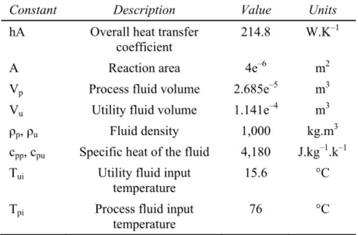
of process fluid and utility fluid respectively. All the values of the model parameters can be found in Zhang et al. (2015). The constants and physical data used in the pilot are given in Table 1.

Heat balance of the process fluid (J.s–1₎

(

)

(

)

p

p p ppdT p u p p pp pi p

ρ V c hA T T ρ F c T T

dt = − + −

Heat balance of the utility fluid (J.s–1₎

(

)

(

)

u

u u pudT u p u u pu ui u

ρ V c hA T T ρ F c T T

dt = − + −

Define the state vector as xT_{= [x}

1, x2]T = [Tp, Tu]T, the

control input T a

u = [ua1, ua2]T = [Fp, Fu]T, the output vector

of measurable variables yT_{= [y}

1, y2] = [Tp, Tu]T, then above

two the equations can be rewritten in the following state-space form:

(

)

(

)

(

)

(

)

a1 1 pi 1 2 1 p a 2 2 ci 2 1 2 u u x T x a x x V u x T x b x x V ⎧ = − + − ⎪⎪ ⎨ ⎪ ₌ ₋ ₊ ₋ ⎪⎩ (11) where 1 1 2 2 p pp p u pu u hA hA a , b , y x , y x . ρ c V ρ c V = = = =

Table 1 Physical data used in the pilot

Constant Description Value Units

hA Overall heat transfer

coefficient 214.8 W.K

–1

A Reaction area 4e–6 _m2

Vp Process fluid volume 2.685e–5 m3

Vu Utility fluid volume 1.141e–4 m3

ρp, ρu Fluid density 1,000 kg.m3

cpp, cpu Specific heat of the fluid 4,180 J.kg–1.k–1

Tui Utility fluid input

temperature

15.6 °C Tpi Process fluid input

temperature 76 °C

5.1.2 Actuator description and Fault scenario

In this work, we need actuators to control flowrate of both process fluid and utility fluid. Pneumatic control valve is employed to act as actuator in this system. The main function of this pneumatic valve is to regulate the flow rate in a pipe line. By application of Bernoulli’s continuous flow law of incompressible fluids, we have:

v P

F C f (X) sg Δ =

where F is flow rate (m3_s–1_{), ΔP is the fluid pressure drop}

across the valve (Pa), sg is specific gravity of fluid and equals 1 for pure water(kgm–3_{), X is the valve opening or}

valve ‘lift’ (X = 1 for max flow), Cv is valve coefficient

(m3_s–1_{) which is given by manufacturer, f(X) is flow}

characteristic which is defined as the relationship between valve capacity and fluid travel through the valve. There are three flow characteristics to choose from: linear valve control; quick opening valve control; equal percentage valve control. For linear valve, f(X) = X, the valve opening is related to stem displacement. In Bartyś et al. (2006) and Roy et al. (1998), a pneumatic control valve has a dynamic model of the type:

2

c a d X₂ dX

p A m μ kX

dt dt

(11)

where Aa is the diaphragm area on which the pneumatic

pressure acts, pc is the pneumatic pressure, m is the mass of

the control valve stem, μ is the friction of the valve stem, k is the spring compliance, and X is the stem displacement or percentage opening of the valve.

Totally, there are 19 kinds of faults that may occur as shown in Bartyś et al. (2006); the causes of each fault are given in Manninen (2012).

Four kinds of fault influencing dynamics of the valve are considered in this paper:

1 fault f1: valve clogging, it occurs when the servomotor stem is blocked by an external event of a mechanical nature. It results in limitation of the piston movement in both direction, and therefore the flow cannot drop below a certain value.

2 fault f2: change of pressure drop across valve, results in P P .′

Δ + Δ

3 fault f3: bellow-seal leakage due to leak, resulting in pcAa + P changed; valve internal leakage is a common

malfunction with industrial control valves. The causes of such leakage are numerous, including damaged plug or seat, insufficient seat load or reduced spring rate. 4 fault f4: control valve diaphragm perforation due to

pinhole cracks in the periphery, resulting in k changed. According to Bartyś et al. (2006), for most parts, single actuator faults are observed in industrial practice whilst multiple faults rarely occur. This characteristic is suited to the situation considered by the scheme proposed in this paper.

5.1.3 Actuator subsystem modelling

Define subscript 1 to denote the actuator of process fluid, then parameters X1, pc1, ΔP1, k1, μ1, F1 represent the opening

percentage of the valve, the pneumatic pressure, and the fluid pressure drop across the valve, the spring compliance process fluid, the friction of the valve stem and flowrate of the process fluid. And denote subscript 2 for the utility fluid, then one gets parameters X2, pc2, ΔP2, k2, μ2, F2 which

represent the same physical meaning for actuator of utility fluid. Since the control valves utilised in this work are linear, then

( )

1 1

( )

2 2

f X =X , f X =X .

In order to evaluate the proposed strategy, the dynamic model should have the form given by (2), so the vector state xa, input u, and output ua are defined as:

[

]

1 2 T a a1 a2 a3 a4 1 dX 2 dX x x x x x X X , dt dt ⎡ ⎤ = _{= ⎢} _⎥ ⎣ ⎦

[

] [

]

T 1 2 c1 c2 u = u u = p p ,

[

]

1 2 T a 1 2 v P 1 v P 2 u F F C X C X , sg sg ⎡ Δ Δ ⎤ = _{= ⎢} _⎥ ⎣ ⎦

[

]

1 2 1 2 3 4 v P v P C c c c c C 0 C 0 . sg sg ⎡ Δ Δ ⎤ = _{= ⎢} ⎥ ⎣ ⎦

The actuator subsystem is then described by four states, two inputs and two outputs, as:

a 1 1 a a a 2 2 a a 0 1 0 0 A 0 m k μ ₀ ₀ 0 0 m m x x u 0 0 0 1 A 0 m k μ 0 0 ₀ ₀ m m u Cx ⎧ ⎡ ⎤ ⎡ ⎤ ⎪ ⎢ ⎥ ⎢ ⎥ ⎪ ⎢₋ ₋ ⎥ ⎢ ⎥ ⎪ ₌⎢ ⎥ ₊⎢ ⎥ ⎪ _⎢ _⎥ _⎢ _⎥ ⎨ _⎢ _⎥ _⎢ _⎥ ⎪ _⎢ _⎥ _⎢ _⎥ ⎪ _⎢ − − _⎥ _⎢ _⎥ ⎣ ⎦ ⎣ ⎦ ⎪ ⎪ ₌ ⎩ (12)

As above description shown, actuator fault may be caused by parameters μ, k, u, Δp, then there are eight related parameters in two actuators: k1, μ1, k2, μ2, pc1, pc2, ΔP1, ΔP2.

The process of RCA is to identify abnormal variations of these eight parameters.

For the sake of RCA purpose, we should rewrite the above dynamic model into fault model as format (3). Therefore, we extend the state, input and output vector as follows:

[

]

T a a1 a2 a3 a4 a5 a6 1 2 1 2 1 2 v 1 v 2 x x x x x x x dX dX P P X X C X C X dt dt sg sg = ⎡ Δ Δ ⎤ = ⎢ ⎥ ⎣ ⎦

[

]

[

]

T 1 2 3 4 5 6 7 8 T 1 1 2 2 c1 c2 1 2 V v v v v v v v v k μ k μ p p P P = = Δ Δ

[

] [

]

T a a1 a2 1 2 a5 a6 1 2 v 1 v 2 u u u F F x x P P C X C X sg sg = = = ⎡ Δ Δ ⎤ = ⎢ ⎥ ⎣ ⎦

[

]

C= 0 0 0 0 1 1

Then, the actuator subsystem is with six states, eight unknown inputs and two outputs. These two outputs are unmeasured which need to be constructed by the global measured outputs. The augmented actuator subsystem is:

( )

8

( )

a a a ai a i i a a x f x g x v u Cx ⎧ = + ⎪ ⎨ ⎪ = ⎩

∑

₍₁₃₎

From (13), there are two outputs. According to Remark 2, in order to guarantee invertibility of (13), there should be two inputs maximum. However, more than two parameters are in (13), therefore, we can only recognise two possible parameters faults simultaneously.

5.2 Invertibility checking and input reconstruction The foundation of the proposed scheme is based on invertibility of an interconnected system. Thus, invertibility

(12)

of individual subsystem is necessary, that means invertibility of both process and actuator subsystem in this work respectively. Besides, the key difficulty and technical challenge is to reconstruct output of actuator system from output of the interconnected system.

5.2.1 Invertibility checking:

To check if the process subsystem, modelled by (11), is invertible, we have to check whether the output differential rank is equal to the number of the inputs. There are two inputs in this work: flowrate of process fluid Fp and flowrate

of utility fluid Fu which are denoted by ua1, ua2 in (11)

respectively. To compute the output differential rank, we first need to derive an explicit expression for the input in terms of the output y by computing the derivatives of y. When it comes to (11), two outputs are temperature of process fluid Tp and utility fluid Tu, which are denoted by

y1, y2 in (11), respectively. As above mentioned, there are

two inputs in this work, the computed output differential rank is equal to the total number of inputs, then the process subsystem is invertible. The same steps could easily be obtained in actuator subsystem. Therefore, the global series system is invertible.

5.2.2 Input reconstruction

Thanks to the invertibility of the process subsystem, we can reconstruct the inputs as a function of the output and its derivatives. From the above equation, an expression for the two inputs can be derived as ua =[ua1 u ] :a2

(

)

(

)

p a1 1 2 1 pi 1 u a2 1 2 1 ci 2 V u y ay ay T y V u y by by T y = − + − = − + −

5.3 Detection observer and RCA observer design 5.3.1 Detection observer design

There are two actuators, then a bank of two detection observers are generated with the form given by (6).

( )

(

)

ai a ai a ai a ai ai ai ˆ ˆ ˆ ˆ x f x g x u K u u 1 i 2 ˆ u Cx ⎧ = + − − ⎪ ≤ ≤ ⎨ = ⎪⎩ (14)

Objective of detection observer is to recognise existence of actuator fault. Therefore, we suppose that all the conditions in the observer are in their nominal values, then if faults occur, ua reconstructed from measured Tp, Tu may be

different from ˆua estimated by observers. After that,

detection residuals rule (7) is employed to produce detection residual r [r= 1 r ].2 Though checking r1, faults in actuator

of process fluid can be detected, and similar method can form r2 for achieving fault detection in actuator of utility

fluid.

5.3.2 RCA observer design

As mentioned before, faults influence μ, k, ΔP, Pc related to

four possible faults resources f1, f2, f3, and f4. Now, let us construct two banks of four observers as (8) for recognising those four possible faults in each control valve.

( )

(

)

(

)

( )

l i i i i i i i j i j j j a a a a l a a i i a a a l i T j j j a i a a i a j j a a 1 j 2,1 i 4 ˆ ˆ ˆ ˆ ˆ ˆ x f x g x θ g x v H u u ˆ ˆ ˆ v 2γ u u Pg x ˆ ˆ u Cx ≠ ≤ ≤ ≤ ≤ ⎧ ₌ ₊ ₊ ₊ ₋ ⎪ ⎪ ⎨ = − ⎪ ⎪ ₌ ⎩

∑

(15) where j_i a

ˆx is the estimated state vector, j i

ˆv is the estimation of root causes and j_i

a

ˆu is the estimated output. The above RCA observers aim at generating two banks of four residuals for those above mentioned fault causes. One bank of residuals are s11, s12, s13, s14, aimed at identifying fault

causes f1, f2, f3, and f4 in actuator of process fluid, the other bank are s21, s22, s23, s24, aimed at identifying fault

causes f1, f2, f3, and f4 in actuator of utility fluid respectively. These residuals are constructed under rules (10), if any of these residuals breaches its threshold, the fault is caused by the corresponding fault causes.

5.4 Simulation results

The simulation results validate the proposed strategy. We first give the operating conditions of the simulation. The input of the inlet flow rate of the utility fluid Fu is

4.22e–5_m3_s–1_{, and inlet flow rate of the process fluid F} p is

4.17e–6_m3_s–1_{. Initial condition for observers supposed to be}

0. Parameters in actuator subsystem are: m = 2 kg, Aa = 0.029 m2, μ = 1,500 Nsm–1 and k = 6,089 Nm–1, Pc for

utility fluid is 1 MPa, 1.2 MPa for process fluid, pressure drop ΔP in utility fluid is 0.6 MPa and 60 kPa in process fluid.

As above mentioned, for most part in practical situation, single fault is observed while multiple faults rarely occur on each actuator. So we consider each actuator is subject to only one fault, then, two faults may occur simultaneously in the actuator subsystem. Two cases are considered to illustrate: noise free and noise corrupted.

5.4.1 Noise free case, fault f3 exists in actuator of process fluid and fault f4 exists in actuator of utility fluid

In this part, two faults are considered. For actuator of process fluid, fault f3 is supposed to occur at 80 s due to unexpected pressure drop across the valve, and for actuator of utility fluid, fault f4 is supposed to occur at 60 s. We supposed that an expected 50 kPa pressure drop adds to the nominal pressure drop across the valve at time 80 s. While because of erosion, the gland packing of the valve may loosen, which leads to stem vibration, a failure value of

(13)

1,000 nm–1_{is added to the spring compliance k. Simulation}

results are listed in Figure 3 to Figure 6.

Figure 3 Reconstructed input F , F from output Tu p p, Tu in

case (a) 0 20 40 60 80 100 0 2 4 6 x 10 -6 Time [s] F low ra te [ m3 /s ]

reconstructed Fp via system inversion

0 20 40 60 80 100 2 4 6 x 10 -5 Time [s] F lo w ra te [ m 3/s ]

reconstructed Fu via system inversion

Figure 4 Detection residual in case (a)

0 20 40 60 80 100 0 5 10 x 10 -7 Time [s]

detection residual r1 for process fluid

0 20 40 60 80 100 0 5 10x 10 -5 Time [s]

detection residual r2 for utility fluid

From Figure 3, after a short transient time, reconstructed inputs ua1=F , up a2 =Fu give an accurate estimation value

to the real inputs ua1 = Fp, ua2 = Fu. At 80 s, the

reconstructed Fp unexpectedly increases, and finally it

stabilises at a new level. This increase implies fault occurs and no further variations illustrate no additional fault occurs. The similar result is obtained in the reconstructed

u

F of utility fluid. The simulation curve indicates that the input reconstruction proposed in this paper is proper for recovering unknown inputs.

As shown in Figure 4, at 80 s and 60 s, the detection residuals (r1, r2) break through their thresholds, respectively.

It implies that at time 80 s, a fault occurs at actuator of process fluid, it takes 0.1 s to detect the fault. While for actuator of utility fluid, at time 60 s, the detection residual r2

no longer remains zero which indicates a fault occurs, fault detection time is 0.2 s.

Figure 5 Residuals for identifying fault cause in process fluid in case (a) 0 20 40 60 80 100 0 1 2 3x 10 -6 Time [s]

RCA residual s11 for process fluid

0 20 40 60 80 100 0 1 2 3x 10 -6 Time [s]

Then, we recognise that, for each actuator, one fault exists. The main contribution of this paper is that we can not only detect and locate the fault, but also can analyse its root cause. Next, we focus on identifying the causes of these two faults.

Figure 5 aims at recognising root cause of the fault at actuator of process fluid. RCA residuals s11, s12, s13, s14 are

designed to recognise four possible candidates: f1, f2, f3, and f4. Detection residual r1 has already implied fault

occurred at 80 s. It is obviously in Figure 5 that, only s13

breaks through and remains above the threshold, which means that fault in actuator of process fluid is caused by fault f3. Isolation time is 0.5 s which is ideal.

(14)

Figure 6 Residuals for identifying fault cause in utility fluid in case (a) 0 20 40 60 80 100 0 1 2 3x 10 -5 Time [s]

RCA residual s21 for utility fluid

0 20 40 60 80 100 0 1 2 3x 10 -5 Time [s]

In Figure 6, RCA residuals s21, s22, s23, s24 are designed to

recognise fault f1, f2, f3, and f4 in actuator of utility fluid. Detection residual r2 in Figure 4 has already implied fault

occurred at 60 s. It is obviously in Figure 6 that only s24

breaches the threshold and never comes back, which means that fault in actuator of utility fluid is caused by fault f4. In this case, isolation time is about 0.2 s. The differences in isolation time is due to magnitude of fault and the effect it has impacted the system.

5.4.2 Noise corrupted case, fault f2 exists in actuator of process fluid and fault f3 exists in actuator of utility fluid

To illustrate the robustness of the proposed scheme, external disturbance or measurement noise is considered in this case. Suppose the output measurement y is corrupted by a coloured noise. The coloured noise is generated with a

second order AR filter excited by a Gaussian white noise with zero mean and unitary variance. The standard deviation of the coloured noise is about 3.5.

Figure 7 Reconstructed input F , F from output Tu p p, Tu in

case (b) 0 20 40 60 80 100 -2 0 2 4 6x 10 -6 Time [s] Flo w ra te [ m3 /s ]

reconstructed Fp via system inversion

0 20 40 60 80 100 0 2 4 6 8x 10 -5 Time [s] Fl ow ra te [ m 3/ s]

reconstructed Fu via system inversion

Figure 8 Detection residual in case (b)

0 20 40 60 80 100 0 2 4 6 x 10 -7 Time [s]

detection residual r1 for process fluid

0 20 40 60 80 100 -1 0 1 2 x 10 -5 Time [s]

detection residual r2 for utility fluid

The same situation as case (a), one fault is considered on each actuator separately. For actuator of process fluid, fault f2 is supposed to be leakage, and reasons that can lead to the leakage are: valve tightness, leaky bushing, and terminals. Fault f3 is supposed in actuator of utility fluid, fault f3 is caused by valve clogging, and it is a commonly encountered fault. If not properly repaired, this kind of fault may cause severe impacts on system performance. Simulation results are demonstrated in Figure 7 to Figure 10.

It can be seen from Figure 7 that although noise exists, the developed input reconstruction techniques can provide reconstructed inputs with a good accuracy. At actuator of process fluid, sudden decrease occurs at 60 s which indicates occurrence of a fault, and it takes 4 s to steady at

(15)

new value. For actuator of utility fluid, the reconstructed value increases from 40 s, and is stable after about 3 s. A fault is detected due to the unexpected increase.

Figure 9 Residuals for identifying fault cause in process fluid in case (a) 0 20 40 60 80 100 0 0.5 1 1.5 2x 10 -6 Time [s]

0 20 40 60 80 100 0 0.5 1 1.5 2x 10 -6 Time [s]

As illustrated in Figure 8, detection residual r1 indicates a

fault in actuator of process fluid at 60 s, it takes 1.2 s to determine the occurrence of the fault. Detection residual r2

refers to a fault in actuator of utility fluid at time 40 s, and it takes 1.5 s to detect it. We can shorten the detection time and detect smaller fault by employing larger gain for the detection observers or adopt a smaller threshold. However, larger gain or larger threshold may fail to detect the fault correctly, since observer with larger gain is too sensitive to noise and smaller threshold may lead to be undistinguished from noise. Therefore a trade between detectability and sensitivity should be made in order to detect the fault correctly. In summary, a small magnitude fault may not be detected within the existence of the noise. Again, after detection of the faults, we have to identify their root causes.

Figure 10 Residuals for identifying fault cause in utility fluid in case (b) 0 20 40 60 80 100 0 1 2 x 10 -5 Time [s]

0 20 40 60 80 100 0 1 2 x 10 -5 Time [s]

We can see from Figure 9 that only RCA residual s12 breaks

through its threshold and remains beyond it, the other three RCA residuals are below their thresholds, then, the fault resource f2 of actuator of process fluid is identified. In case of RCA residuals for actuator of utility fluid in Figure 10, only s23 is beyond its threshold which verifies the

occurrence of fault cause f3.

From the above simulation results, we can see that the proposed strategy is able to detect and locate a fault correctly, and RCA for each detected fault is achieved with a good accuracy. Encouraging simulation results are obtained thanks to the robustness of the proposed scheme.

6 Conclusions

The main contribution of this paper lies on the integration of both system level and component level-based FDI approaches to facilitate FDI and RCA of subcomponents actuators. A left invertible interconnected nonlinear system

(16)

structure is developed which guarantees that faults occurring in actuator subsystem will affect the measured output of the global system uniquely and distinguishably. The new system structure, together with the fault diagnosis algorithm, is the first to emphasise the importance of RCA of field devices fault, as well as the influences of local internal dynamics on the global dynamics. Since local measurement is assumed inaccessible and estimated from global output, it is more realistic due to remote distance or physical availability considerations for an industrial application. Therefore, this approach not only completes the theory but is also of great importance to narrow the gap between industry and academia. Simulated results are included to demonstrate the applicability and robustness of the proposed method and encouraging results are obtained.

For future work, one interesting research direction is to develop an input estimator which avoids using computation of successive derivatives of outputs to estimate the inputs of the process subsystem. It is because successive derivatives are considered unrealistic in practical applications since measurements suffer noise and disturbances. Another consideration is to approach the problem of parameter observability and diagnosability at local subsystem from the view point of global output, and to investigate a strategy of multi parameters identification.

Acknowledgements

The present work is supported by National Natural Science Foundation of China No. 61540067 and Guizhou Big Data Collaborative Research Innovation Center, No. Qian jiao He Xie Tong Chuang Xin Zi 2014 (02).

References

Bartyś, M., Patton, R., Syfert, M., de las Heras, S. and Quevedo, J. (2006) ‘Introduction to the DAMADICS actuator FDI benchmark study’, Control Engineering Practice, Vol. 14, No. 6, pp.577–596.

Benaïssa, W., Gabas, N., Cabassud, M., Carson, D., Elgue, S. and Demissy, M. (2008) ‘Evaluation of an intensified continuous heat-exchanger reactor for inherently safer characteristics’,

Journal of Loss Prevention in the Process Industries, Vol. 21,

No. 5, pp.528–536.

Blesa, J., Rotondo, D., Puig, V. and Nejjari, F. (2014) ‘FDI and FTC of wind turbines using the interval observer approach and virtual actuators/sensors’, Control Engineering Practice, Vol. 24, No. 1, pp.138–155.

Chen, W., Chen, W., Saif, M. and Saif, M. (2005) ‘An actuator fault isolation strategy for linear and nonlinear systems’,

2005 American Control Conference, Portland, USA,

pp.3321–3326.

Ding, H. and Zhao, J. (2014) ‘Characteristic analysis of valve-pump parallel connection in a variable frequency hydraulic system’, International Journal of Modelling,

Identification and Control, Vol. 21, No. 3, pp.223–236.

Edelmayer, A., Bokor, J., Szigzabo, Z. and Seti, F. (2004) ‘Input reconstruction by means of system inversion: a geometric approach to fault detection and isolation in nonlinear systems’, International Journal of Applied Mathematics and

Computer Science, Vol. 14, No. 2, pp.189–199.

Edwards, C., Alwi, H. and Tan, C.P. (2012) ‘Sliding mode methods for fault detection and fault tolerant control with application to aerospace systems’, International Journal of

Applied Mathematics and Computer Science, Vol. 22, No. 1,

pp.109–124.

Farza, M., Saad, M.M., Liu, F. and Targui, B. (2007) ‘Generalised observers for a class of non-linear systems’, International

Journal of Modelling, Identification and Control, Vol. 53,

No. 2, pp.24–32.

Fragkoulis, D., Roux, G. and Dahhou, B. (2011) ‘Detection, isolation and identification of multiple actuator and sensor faults in nonlinear dynamic systems: application to a waste water treatment process’, Applied Mathematical Modelling, Vol. 35, No. 1, pp.522–543.

Isidori, A. (1995) Nonlinear Control Systems, 3rd ed., Springer, Berlin.

Li, Z. and Dahhou, B. (2006) ‘Parameter intervals used for fault isolation in non-linear dynamic systems’, International

Journal of Modelling, Identification and Control, Vol. 1,

No. 3, pp.215–229.

Li, Z. and Dahhou, B. (2008) ‘A new fault isolation and identification method for nonlinear dynamic systems: application to a fermentation process’, Applied Mathematical

Modelling, Vol. 32, No. 12, pp.2806–2830.

Maksimov, V. and Pandolfi, L. (2001) ‘Dynamical reconstruction of unknown inputs in nonlinear differential equations’,

Applied Mathematics Letters, Vol. 14, No. 6, pp.725–730.

Manaa, I., Barhoumi, N. and M’Sahli, F. (2015) ‘Unknown inputs observers design for a class of nonlinear switched systems’,

International Journal of Modelling, Identification and

Control, Vol. 23, No. 1, pp.45–54.

Manninen, T. (2012) Fault Simulator and Detection for a Process

Control Valve, PhD thesis, Aalto University.

Martínez-Guerra, R., Mata-Machuca, J.L. and Rincón-Pasaye, J.J. (2013) ‘Fault diagnosis viewed as a left invertibility problem’, ISA Transactions, Vol. 52, No.5, pp.652–661. McGhee, J., Henderson, I.A. and Baird, A. (1997) ‘Neural

networks applied for the identification and fault diagnosis of process valves and actuators’, Measurement, Vol. 20, No. 4, pp.267–275.

Methnani, S. (2013) ‘Actuator and sensor fault detection, isolation and identification in nonlinear dynamical systems, with an application to a waste water treatment plant’, Journal of

Computer Engineering and Informatics, Vol. 1, No. 4,

pp.112–125.

Nagy-Kiss, A.M. and Schutz, G. (2013) ‘Estimation and diagnosis using multi-models with application to a wastewater treatment plant’, Journal of Process Control, Vol. 23, No. 10, pp.1528–1544.

Persis, C.D. and Isidori, A. (2001) ‘A geometric approach to nonlinear fault detection and isolation’, IEEE Transactions on

Automatic Control, Vol. 46, No. 6, pp.1–22.

Pinheiro, V. and Araújo, R.E. (2013) ‘Evaluation of applicability of system inversion to fault detection and isolation on switched power converters’, Conference on Control and