CFD/CSD grid interfacing of three-dimensional surfaces by inverse isoparametric maping

(1)

CFD/CSD Grid Interfacing of Three-Dimensional Surfaces

by Inverse Isoparametric Mapping

by

Pong Kwong Lee

B.S., Aeronautical and Astronautical Engineering (1999) B.S., Computer Science (1999)

University of Illinois at Urbana-Champaign

Submitted to the Department of Aeronautics and Astronautics in partial fulfillment of the requirements for the degree of

MASTER OF SCIENCE

at the

MASSACHUSETTS INSTITUTE OF TECHNOLOGY

June 2001

@

Author

Department of Aeronautics and Astronautics May 25, 2001

Certified by

Cars E. S. Cesnik Assistant Professor of Aeronautics and Astronautics Thesis Supervisor

Accepted by

MASSACHUSETTS INSTITUTE OF TECHNOLOGY

SEP

11 2001

Wallace E. Vander Velde Professor of Aeronautics and Astronautics Chair, Committee on Graduate Students

(2)

(3)

CFD/CSD Grid Interfacing of Three-Dimensional Surfaces by Inverse

Isoparametric Mapping

by

Pong Kwong Lee

Submitted to the Department of Aeronautics and Astronautics on May 25, 2001, in partial fulfillment of the

requirements for the degree of Master of Science

Abstract

To effectively transfer data between Computational Fluid Dynamics (CFD) and Computa-tional Structural Dynamics (CSD) grids in the field of ComputaComputa-tional Aeroelasticity requires an effective method that must provide a smooth interfacing between the two grids and han-dles a variety of variables and functional forms. A finite-element approach using the Inverse Isoparametric Mapping (IM) method was found to provide an excellent alternative to han-dle such grid interfacing for three-dimensional (3D) surfaces, such as wings and fuselages. The IIM method is a one-to-one mapping that utilizes the same shape functions to inter-polate both the geometric and field quantities (i.e. displacements, rotations, or loads).

The interpolation of displacements and loads using the IIM method is developed using both 3- and 6-node triangles, which provide a linear and quadratic interpolation, respec-tively. The IIM method was found to provide a suitable interfacing solution to the problem with both types of triangular elements. The 6-node triangle provides a smoother displace-ment interpolation than the 3-node triangle, while the 3-node triangle provides a better interpolation of loads. To account for the curvatures of different geometries in 3D surfaces, a method based on the rotations with quaternions is used to provide proper element trans-formations and sets up a local coordinate axis system on each triangular elements to allow local interpolation of the data within that element.

The study of accuracy and effectiveness of the IIM method is conducted here with some simple analytical test cases and three aeroelastic representative test cases: AGARD 445 wing, the lower wing of a generic hypersonic vehicle, and the fusalage of a generic hypersonic vehicle. For all test cases, the IIM method was found to provide an excellent interfacing of data comparable to global methods such as the Multiquadric-Biharmonic (MQ) and the Thin-Plate Spline (TPS) methods. The IIM method tends to provide a consistent interpolation of data throughout the entire grid, whereas the MQ and TPS methods tend to lose smoothness and accuracy near the edges and boundaries of the grid. The IIM method is found to be a promising method for most aeroelastic applications. As a local interpolation scheme, the IIM method is shown to be both simple to implement and robust in interpolating 3D surfaces with curvatures.

Thesis Supervisor: Carlos E. S. Cesnik

(4)

(5)

Acknowledgments

I would like to express my appreciation and gratitude to my advisor, Professor Carlos Cesnik, for introducing this research topic to me and providing me with the guidance, advice, and support throughout the project. I must say that he is solely responsible for introducing me to the exciting field of computational aeroelasticity, which I overlooked in my undergraduate years. Special thanks to Professor John Dugundji of TELAC who provided me with some valuable insights in this field throughout the course of my project.

Many thanks to David Kenwright and Bob Haimes of FDRL, who spent much of their valuable time helping me with CFD test cases. It would have been impossible for me to complete many of my complex application test cases without their help throughout the year. I have to mention that I learned a great deal about Computational Fluid Dynamics

while working with them.

I am grateful to Debashis Sahoo of TELAC, who provided me with timely help in running test cases using NASTRAN. Not only did he provide me with valuable inputs running the finite element analyses, his willingness in allowing me to use his computer and resources help me through most of the critical stages of the project.

I must also thank Dennis Burianek of TELAC. Dennis provided me with the guidance and support in using the computers and numerous software packages in TELAC. He also introduced me to the use of LATEX and provided me with the guidance and advice on using this powerful tool with which this thesis is written.

I would like to thank Seth Kessler who also provided me with valuable technical advices during some critical stages of my project.

I must thank my parents and my younger sister for providing me with the support and encouragement to attend MIT in Cambridge, MA for my graduate education. They helped me a great deal in making my transition from my undergraduate school in Champaign, IL to Massaschusetts.

Lastly, special thanks to the Department of Aeronautics and Astronautics at MIT for providing me with a fellowship which funded the first half of my project and Professor Nancy Leveson of SERL for providing me with the funding to work on her software projects during the second half, while I still managed to have time for this.

(6)

(7)

List of Figures

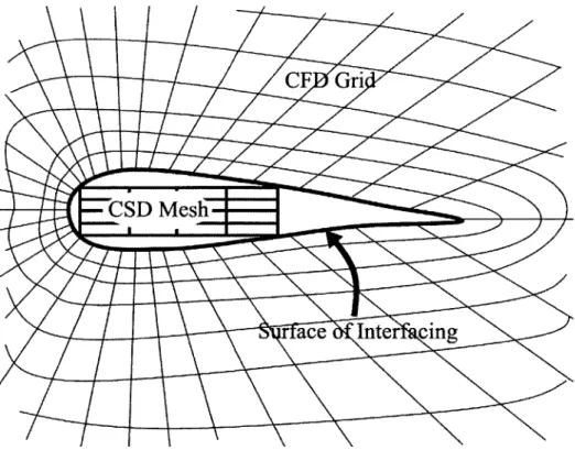
1-1 The surface of interfacing between a CFD grid and a CSD mesh of an airfoil 24

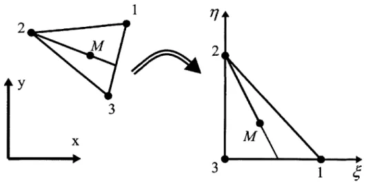
2-1 The mapping from a global to a natural coordinate system using the Inverse

Isoparametric Mapping (IIM) . . . . 32

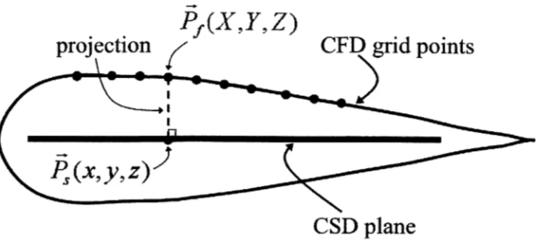
2-2 Rigid body rotation between a CFD point and a CSD element . . . . 34

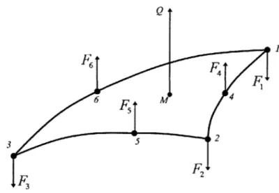
2-3 The interpolation of loads using IIM with a 3-node triangle . . . . 37

2-4 The interpolation of loads using IIM with a 6-node triangle . . . . 38

2-5 A 3-node triangle defined in the natural coordinate system with out-of-plane displacem ents . . . . 39

2-6 A 3-node triangle defined in the natural coordinate system with out-of-plane displacements and rotations about both axes . . . . 42

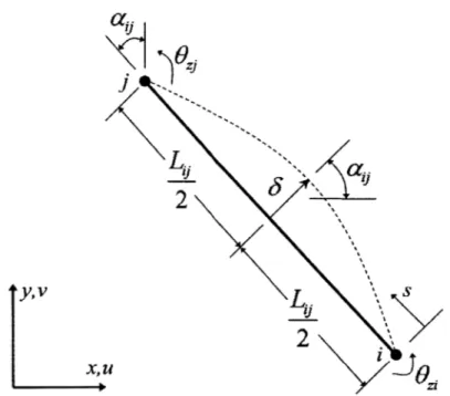
2-7 Displacement at a side of a 3-node triangle produced by the drilling degrees of freedom given at two nodes . . . . 43

2-8 A 6-node triangle defined in the natural coordinate system with out-of-plane displacem ents . . . . 45

2-9 Rotations with quaternions applied to a point using a unit vector and a rotation angle . . . . 46

3-1 The shortest distance between a given CFD point and a CSD element . . . 53

3-2 Information for determining whether a given CFD point lies inside a 3-node triangle . . . . 55

3-3 Method for determining whether a given CFD point lies inside a 6-node triangle 56 3-4 Definition of an iterating line for a 6-node triangle . . . . 61

(12)

3-6 The overlapping regions between the interpolation and extrapolation of

dis-placem ents . . . . 67

3-7 A CFD point without an associated CSD element . . . . 68

4-1 Test 1 - Interpolation of Axisymmetric Displacements on a 3D Surface . . . 80

4-2 Test 2 - Displacement Interpolation on a Deflected 3D Surface . . . . 81

4-3 Test 3 - Interpolation of a Constant Load Distribution on a Flat Surface . . 82

4-4 Test 4 - Interpolation of an Axisymmetric Load Distribution on a Flat 2D Surface . . . . 83

4-5 Test 5 - Interpolation of an Axisymmetric Load Distribution on a 3D Surface 84 4-6 Test 6 - Displacement Extrapolation on a Deflected 3D Surface . . . . 85

4-7 Test 7 - Extrapolation of a Constant Load Distribution on a Flat Surface . 86 4-8 Test 8 - Interpolation of Rotations . . . . 87

4-9 Test 8 - Rotations about the x-axis . . . . 88

4-10 Test 8 - Rotations about the y-axis . . . . 89

4-11 Test 8 - Rotations about the z-axis . . . . 90

4-12 Test 9 - Displacement Interpolation on a 3D Surface with a Sharp Curvature 91 4-13 Test 10 - Displacement Interpolation on a 3D Surface - Internal Anomalous P oints . . . . 92

4-14 Test 11 - Large Displacement Interpolation on a 3D Surface . . . . 93

4-15 Test 12 - Interpolation of a One-Cycle Sinusoidal Displacement on a 2D Surface 94 4-16 Test 13 - Interpolation of a Three-Cycle Sinusoidal Displacement on a 2D Surface . . . . 95

4-17 Test 14 - Interpolation of a Three-Cycle Sinusoidal Displacement on a 3D Surface . . . . 96

4-18 Test 15 - Interpolation of Displacements on a 2D Surface . . . . 97

4-19 Test 15 - Interpolation of Rotations on a 2D Surface . . . . 98

4-20 AGARD 445 wing . . . . 99

4-21 AGARD 445 wing CSD mesh mode shape 1 . . . . 100

4-22 AGARD 445 wing CSD mesh mode shape 2 . . . . 101

4-23 AGARD 445 wing CSD mesh mode shape 3 . . . . 102

(13)

4-25 4-26 4-27 4-28 4-29 4-30 4-31 4-32 4-33 4-34 4-35 4-36 4-37 4-38 4-39 4-40 4-41 4-42

AGARD 445 wing CSD mesh mode shape 5 ... Hypersonic lower wing ...

Hypersonic lower wing CSD mesh mode shape 1 Hypersonic lower wing CSD mesh mode shape 2 Hypersonic lower wing CSD mesh mode shape 3 Hypersonic lower wing CSD mesh mode shape 4 Hypersonic lower wing CSD mesh mode shape 5 Hypersonic lower wing CSD mesh mode shape 6 Hypersonic lower wing CSD mesh mode shape 7 Hypersonic fuselage . . . . Hypersonic fuselage CSD mesh mode shape 1 Hypersonic fuselage CSD mesh mode shape 2 Hypersonic fuselage CSD mesh mode shape 3 Hypersonic fuselage CSD mesh mode shape 4 Hypersonic fuselage CSD mesh mode shape 5 Hypersonic fuselage CSD mesh mode shape 6 Hypersonic fuselage CSD mesh mode shape 7 Hypersonic fuselage CSD mesh mode shape 8

. . . . 104 . . . . 10 5 . . . . 10 6 . . . . 10 6 . . . . 10 7 . . . . 10 7 . . . . 10 8 . . . . 10 8 . . . . 10 9 . . . . 110 . . . .111 . . . .111 . . . . 112 . . . . 112 . . . . 113 . . . . 113 . . . . 114 . . . . 114

5-1 Inverse Isoparametric Mapping (3-node triangle) results for Test 1 . . . . . 141 5-2 Inverse Isoparametric Mapping (6-node triangle) results for Test 1 . . . . . 5-3 Absolute errors between IIM interpolated and theoretical displacements for

Test 1 ... ... ... ...

5-4 Multiquadric Biharmonic results for Test 1 . . . . 5-5 Thin-Plate Spline results for Test 1 . . . . 5-6 Absolute errors between MQ/TPS interpolated and theoretical displacements

for T est 1 . . . . 5-7 Inverse Isoparametric Mapping (3-node triangle) results for Test 2 . . . . . 5-8 Inverse Isoparametric Mapping (6-node triangle) results for Test 2 . . . . . 5-9 Absolute errors between IIM interpolated and theoretical displacements for

Test 2 ... .. ...

5-10 Multiquadric Biharmonic results for Test 2 . . . . 142 143 144 145 146 147 148 149 150

(14)

5-11 Thin-Plate Spline results for Test 2 . . . . 151

5-12 Absolute errors between MQ/TPS interpolated and theoretical displacements for Test 2 . . . . 152

5-13 IIM/TPS (6-node triangle with 30% patches) results for Test 6 . . . . 153

5-14 IIM/TPS (6-node triangle with 50% patches) results for Test 6 . . . . 154

5-15 IIM/TPS (6-node triangle without patches) results for Test 6 . . . . 155

5-16 Absolute errors between IIM/TPS (with patches) interpolated/extrapolated and theoretical displacements for Test 6 . . . . 156

5-17 Absolute errors between IIM/TPS (without patches) interpolated/extrapolated and theoretical displacements for Test 6 . . . . 157

5-18 Multiquadric Biharmonic results for Test 6 . . . . 158

5-19 Thin-Plate Spline results for Test 6 . . . . 159

5-20 Absolute errors between MQ/TPS interpolated/extrapolated and theoretical displacements for Test 6 . . . . 160

5-21 IIM (3-node 9 d.o.f. triangle) interpolated displacement results for Test 8 . 161 5-22 IIM (3-node 9 d.o.f. triangle) interpolated rotation about the x-axis results for Test 8 . . . . 162

5-23 IIM (3-node 9 d.o.f. triangle) interpolated rotation about the y-axis results for Test 8 . . . . 163

5-24 IIM (3-node 9 d.o.f. triangle) interpolated rotation about the z-axis results for Test 8 . . . . 164

5-25 Absolute error between IIM (3-node 9 d.o.f. triangle) interpolated and theo-retical displacements and rotations for Test 8 . . . . 165

5-26 Absolute error between IIM (3-node 9 d.o.f. triangle) interpolated and theo-retical rotations for Test 8 . . . . 166

5-27 IIM (3-node 3 d.o.f. triangle) interpolated displacement results for Test 8 167 5-28 IIM (6-node 6 d.o.f. triangle) interpolated displacement results for Test 8 168 5-29 Absolute error between IIM interpolated and theoretical displacements for Test 8 .... ... ... .. ... ... ... 169

5-30 IIM (6-node 6 d.o.f. triangle) interpolated rotation about the x-axis results for Test 8 . . . . 170

(15)

5-33 Absolute error between IIM (6-node 6 d.o.f. triangle) interpolated and theo-retical rotations for Test 8 . . . . 173 5-34 Absolute error between IIM (6-node 6 d.o.f. triangle) interpolated and

theo-retical rotations about the z axis for Test 8 . . . . 174 5-35 Inverse Isoparametric Mapping (3-node triangle) results for Test 9 . . . . . 175 5-36 Inverse Isoparametric Mapping (6-node triangle) results for Test 9 . . . . . 176 5-37 Absolute errors between IIM interpolated and theoretical displacements for

Test 9 ... .. ... 177 5-38 Thin-Plate Spline results for Test 9 . . . . 178 5-39 Absolute errors between TPS interpolated and theoretical displacements for

Test 9 ... .. ... 179 5-40 Inverse Isoparametric Mapping (3-node triangle) results for Test 10 . . . . . 180 5-41 Inverse Isoparametric Mapping (3-node triangle) results with internal

extrap-olation for Test 10 . . . . 181 5-42 Inverse Isoparametric Mapping (6-node triangle) results for Test 10 . . . . . 182 5-43 Absolute errors between IIM (3-node triangle) interpolated and theoretical

displacements for Test 10 . . . . 183 5-44 Absolute errors between IIM (6-node triangle) interpolated and theoretical

displacements for Test 10 . . . . 184 5-45 Thin-Plate Spline results for Test 10 . . . . 185 5-46 Absolute errors between TPS interpolated and theoretical displacements for

Test 10 ... .... ... 186

5-47 Inverse Isoparametric Mapping (3-node triangle) results for Test 11 . . . . . 187 5-48 Inverse Isoparametric Mapping (6-node triangle) results for Test 11 . . . . . 188 5-49 Absolute errors between IIM interpolated and theoretical displacements for

Test 11 ... ... 189 5-50 Multiquadric Biharmonic results for Test 11 . . . . 190 5-51 Thin-Plate Spline results for Test 11 . . . . 191

(16)

5-52 Absolute errors between MQ/TPS interpolated and theoretical displacements for Test 11 . . . . 192 5-53 Inverse Isoparametric Mapping (3-node triangle) results for Test 12 . . . . . 193 5-54 Inverse Isoparametric Mapping (6-node triangle) results for Test 12 . . . . . 194 5-55 Absolute errors between IIM interpolated and theoretical displacements for

Test 12 ... .... ... 195

5-56 Inverse Isoparametric Mapping (3-node triangle) results for Test 13 . . . . . 196 5-57 Inverse Isoparametric Mapping (6-node triangle) results for Test 13 . . . . . 197 5-58 Absolute errors between IIM interpolated and theoretical displacements for

Test 13 . . . . 198

5-59 Inverse Isoparametric Mapping (3-node triangle) results for Test 14 . . . . . 199 5-60 Inverse Isoparametric Mapping (6-node triangle) results for Test 14 . . . . . 200 5-61 Absolute errors between IIM interpolated and theoretical displacements for

Test 14 . . . . 201 5-62 IIM (9 d.o.f. 3-node triangle) interpolated displacement results for Test 15 . 202 5-63 IIM (9 d.o.f. 3-node triangle) interpolated tangent of the rotation about the

x-axis results for Test 15 . . . . 203 5-64 IIM (9 d.o.f. 3-node triangle) interpolated tangent of the rotation about the

y-axis results for Test 15 . . . . 204 5-65 IIM (6 d.o.f. 6-node triangle) interpolated displacement results for Test 15 . 205 5-66 Absolute error between IIM interpolated and theoretical displacements for

T est 15 . . . . 206 5-67 Absolute error between IIM (9 d.o.f. 3-node triangle) interpolated and

theo-retical tangent of the rotations for Test 15 . . . . 207 5-68 Inverse Isoparametric Mapping (3-node triangle) results for AGARD 445

wing, mode shape 1 . . . . 208 5-69 Inverse Isoparametric Mapping (3-node triangle) results for AGARD 445

wing, mode shape 2 . . . . 209 5-70 Inverse Isoparametric Mapping (3-node triangle) results for AGARD 445

wing, mode shape 3 . . . . 210 5-71 Inverse Isoparametric Mapping (3-node triangle) results for AGARD 445

(17)

5-72 Inverse Isoparametric Mapping wing, mode shape 5 . . . . 5-73 Inverse Isoparametric Mapping wing, mode shape 1 . . . . 5-74 Inverse Isoparametric Mapping wing, mode shape 2 . . . . 5-75 Inverse Isoparametric Mapping wing, mode shape 3 . . . . 5-76 Inverse Isoparametric Mapping wing, mode shape 4 . . . . 5-77 Inverse Isoparametric Mapping wing, mode shape 5 . . . .

(3-node triangle) results for AGARD 445

(6-node (6-node (6-node (6-node (6-node .t.r. . . .. . . . . . triangle) results for .t.r. . . .. . . . . . triangle) results for

triangle) results for

AGARD 445

AGARD 445 AGARD 445 . . . . 2 1 7 5-78 Thin-Plate Spline results fo

Thin-Plate Spline results fo Thin-Plate Spline results fo Thin-Plate Spline results fo Thin-Plate Spline results fo 5-83 IIM/TPS IIM/TPS IIM/TPS IIM/TPS IIM/TPS IIM/TPS IIM/TPS IIM/TPS IIM/TPS IIM/TPS IIM/TPS IIM/TPS IIM/TPS IIM/TPS (3-node triangle) (3-node triangle) (3-node triangle) (3-node triangle) (3-node triangle) (3-node triangle) (3-node triangle) (6-node triangle) (6-node triangle) (6-node triangle) (6-node triangle) (6-node triangle) (6-node triangle) (6-node triangle)

r AGARD 445 wing, mode shape r AGARD 445 wing, mode shape r AGARD 445 wing, mode shape r AGARD 445 wing, mode shape r AGARD 445 wing, mode shape results for hypersonic lower wing, results for hypersonic lower wing, results for hypersonic lower wing, results for hypersonic lower wing, results for hypersonic lower wing, results for hypersonic lower wing, results for hypersonic lower wing, results for hypersonic lower wing, results for hypersonic lower wing, results for hypersonic lower wing, results for hypersonic lower wing, results for hypersonic lower wing, results for hypersonic lower wing, results for hypersonic lower wing,

1 . . . . 218 2.. 3.. 4.. 5.. mode mode mode mode mode mode mode mode mode mode mode mode mode shape shape shape shape shape shape shape shape shape shape shape shape shape mode shape 5-97 Thin-Plate Spline results for hypersonic lower wing, mode shape 1

219 220 221 222 223 223 224 224 225 225 226 226 227 227 228 228 229 229 230 212 213 214 215 216 5-79 5-80 5-81 5-82 5-84 5-85 5-86 5-87 5-88 5-89 5-90 5-91 5-92 5-93 5-94 5-95 5-96

(18)

5-98 Thin-Plate Spline results for hypersonic lower wing, mode 5-99 Thin-Plate Spline results for hypersonic lower wing, mode 5-10OThin-Plate Spline results for hypersonic lower wing, mode 5-10IThin-Plate Spline results for hypersonic lower wing, mode 5-102Thin-Plate Spline results for hypersonic lower wing, mode 5-103Thin-Plate Spline results for hypersonic lower wing, mode 5-104IIM/TPS (3-node triangle) results for hypersonic fuselage, 5-105IIM/TPS (3-node triangle) results for hypersonic fuselage, 5-106IIM/TPS (3-node triangle) results for hypersonic

5-107IIM/TPS (3-node triangle) results for hypersonic 5-108IIM/TPS (3-node triangle) results for hypersonic 5-109IM/TPS (3-node triangle) results for hypersonic 5-110IM/TPS (3-node triangle) results for hypersonic 5-111IIM/TPS (3-node triangle) results for hypersonic 5-112Thin-Plate Spline results for hypersonic fuselage, 5-113Thin-Plate Spline results for hypersonic fuselage, 5-114Thin-Plate Spline results for hypersonic fuselage, 5-115Thin-Plate Spline results for hypersonic fuselage, 5-116Thin-Plate Spline results for hypersonic fuselage, 5-117Thin-Plate Spline results for hypersonic fuselage, 5-118Thin-Plate Spline results for hypersonic fuselage, 5-119Thin-Plate Spline results for hypersonic fuselage, 5-12OThe front views of the hypersonic fuselage . . . . 5-121IIM/TPS (6-node triangle) results for hypersonic 5-122IIM/TPS (6-node triangle) results for hypersonic 5-123CPU time requirements for the interpolation of a

fuselage, fuselage, fuselage, fuselage, fuselage, shape shape shape shape shape shape mode mode mode mode mode mode mode fuselage, mode mode mode mode mode mode mode mode mode 2 3 4 5 6 7 sh sh sh sh sh sh sh sh shape shape shape shape shape shape shape shape

fuselage, mode shE

. . .. ... 230 . . .. ... 231 . . . . . 231 . . . . . 232 232 . . .. ... 233 ape1. . 234 ape2. . 234 ape3. . 235 ape 4. . 235 ape 5. . 236 ape6. . 236 ape7. . 237 ape8. . 237 . . . . . 238 . . . . . 238 . . . . . 239 . . . . . 239 . . . . . 240 . . . . . 240 . . . . . 241 . . . . . 241 . . . . . 242 pe 8 . . 243 fuselage, mode shape 8 . . 2D surface of Test 1 using the IIM m ethod . . . . 5-124Memory requirements for the interpolation of a 2D surface of Test 1 using the IIM m ethod . . . . 5-125CPU time requirements for the interpolation of a 3D surface of Test 1 using

IIM , M Q , and TPS . . . . 244

245

246

(19)

5-126Memory requirements for the interpolation of a 3D surface of Test 1 using IIM , M Q, and TPS . . . . 248 5-127CPU time requirements for the extrapolation of a 3D surface of Test 6 using

IIM /TPS and TPS . . . . 249 5-128Memory requirements for the extrapolation of a 3D surface of Test 6 using

IIM/TPS and TPS . . . . 250

6-1 Point force distribution on the CFD grid points for Test 3 . . . . 260 6-2 Point force distribution on the CSD nodal points for Test 3 . . . . 261 6-3 Displacements from the FEA solution based on the CFD grid points with

their corresponding point forces for Test 3 . . . . 262 6-4 Displacements from the FEA solution based on the CSD nodal points with

their corresponding interpolated point forces using IIM with 3-node triangles for Test 3 . . . . 263

6-5 Displacements from the FEA solution based on the CSD nodal points with their corresponding interpolated point forces using IIM with 6-node triangles for Test 3 . . . . 264 6-6 Absolute error plot of the displacements for the two IIM implementations

comparing the FEA solution for the CFD grid and the CSD mesh for Test 3 265 6-7 Point force distribution on the CFD grid points for Test 4 . . . . 266 6-8 Point force distribution on the CSD nodal points for Test 4 . . . . 267 6-9 Displacements from the FEA solution based on the CFD grid points with

their corresponding interpolated point forces using IIM with 3-node triangles for T est 4 . . . . 269 6-11 Displacements from the FEA solution based on the CSD nodal points with

6-12 Absolute error plot of the displacements for the two IIM implementations comparing the FEA solution for the CFD grid and the CSD mesh for Test 4 271 6-13 Point force distribution on the CFD grid points for Test 5 . . . . 272

(20)

6-14 Point force distribution on the CSD nodal points for Test 5 . . . . 273 6-15 Displacements from the FEA solution based on the CFD grid points with

their corresponding point forces for Test 5 . . . . 274 6-16 Displacements from the FEA solution based on the CSD nodal points with

6-17 Displacements from the FEA solution based on the CSD nodal points with their corresponding interpolated point forces using IIM with 6-node triangles forTest5 . . . .. .. .... .. . . . .. . . . . 276

6-18 Absolute error plot of the displacements for the two IIM implementations comparing the FEA solution for the CFD grid and the CSD mesh for Test 5 277 6-19 Point force distribution on the CFD grid points for Test 7 . . . . 278 6-20 Point force distribution on the CSD nodal points for Test 7 . . . . 279 6-21 Displacements from the FEA solution based on the CFD grid points with

their corresponding interpolated point forces using IIM with 3-node triangles for Test 7 . . . . 281 6-23 Displacements from the FEA solution based on the CSD nodal points with

their corresponding interpolated point forces using IIM with 6-node triangles for Test 7 . . . . 282 6-24 Point force distribution on the CFD grid points for for hypersonic lower wing 283 6-25 Point force distribution on the CSD nodal points for hypersonic lower wing 284 6-26 Displacements from a FEA based on the loads on the CFD grid points for

the hypersonic lower wing . . . . 285 6-27 Displacements from a FEA based on the interpolated loads using JIM with

3-node triangles on the CSD nodal points for the hypersonic lower wing . . 286

6-28 Displacements from a FEA based on the interpolated loads using IIM with 6-node triangles on the CSD nodal points for the hypersonic lower wing . . 287

(21)

List of Tables

5.1 Statistical Summary of Test 6 for the interpolated regions . . . . 120

5.2 Statistical Summary of Test 6 for the overlapped regions . . . . 120

5.3 Statistical Summary of Test 6 for the extrapolated regions . . . . 121

5.4 Statistical Summary of Test 12 . . . . 126

5.5 Statistical Summary of Test 13 . . . . 127

5.6 Statistical Summary of Test 14 . . . . 128

5.7 Comparison of maximum deflections for the AGARD 445 wing mode shapes 131 5.8 Comparison of performance between IIM, MQ, and TPS for Test 1 . . . . . 136

5.9 Comparison of performance between IIM/MQ, IIM/TPS, MQ, and TPS for T est 6 . . . . 136

5.10 Comparison of performance between IIM, MQ, and TPS for AGARD 445 wing137 5.11 Comparison of performance between IIM/MQ, IIM/TPS, MQ, and TPS for hypersonic lower wing . . . . 137

5.12 Performance of IIM with 3-node and 6-node triangles on various grid sizes of Test 1 with a 2D surface . . . . 138

5.13 Performance of IIM, MQ, and TPS on various grid sizes of Test 1 with a 3D surface . . . . 139

5.14 Performance of IIM/TPS with 3-node and 6-node triangles on various grid sizes of Test 6 . . . . 140

6.1 Comparison of force, moment, and work for Test 3 . . . . 257

6.4 Comparison of force, moment, and work for Test 7 . . . . 259

(22)

(23)

Chapter 1 Introduction

1.1 Motivation

Historically, in the design and development process of an aircraft, the high-fidelity analyses of fluids and structures are usually performed relatively independent from one another. It is desired and, in most cases, necessary to accurately account for the interaction between fluids and structures when designing new generation aircraft. Due to the flexibility of the struc-tures of an aircraft in flight, the coupling between Computational Fluid Dynamics (CFD) and Computational Structural Dynamics (CSD) must be carefully considered in order to capture the complex interactions of unsteady aerodynamics and structural dynamics. There are three primary classes of analyses in the field of Computational Aeroelasticity (CAE)

[1]. In the fully coupled analysis, both the fluid and structural equations are combined into one, and the solutions are solved simultaneously. Any interactions between aerodynamics and structural dynamics are integrated into the governing equations. Due to the complexity in solving the equations, the fully coupled analysis is not widely available. In the loosely and closely coupled analyses, however, the fluid and structural solutions are solved quite independently. The interactions between CFD and CSD, which are limited to the passage of surface loads and surface deformation information, must be integrated through the in-terfacing of grid data during each iteration. Since it is very unlikely that all CSD nodes and CFD grid points will coincide with one another, interpolation and extrapolation are necessary to interface the data flow between the two grids in both the loosely and closely coupled analyses.

(24)

Figure 1-1: The surface of interfacing between a CFD grid and a CSD mesh of an airfoil

the fully coupled analysis, because they provide the freedom for analysts and engineers to perform the fluid and structural analyses independently from one another in the design and development process of an aircraft. The interactions at the fluid/structure boundary are performed through the use of interpolation and extrapolation methods that are independent from the choice of methods used in the fluid or structural analyses.

CFD and CSD grid interfacing is usually considered on the infinitely thin 3D surface where the CFD grid and the CSD mesh meet each other as shown in Figure 1-1. The main difficulty in transferring data between the CFD grid and the CSD mesh lies in the fact that the grids are different from one another. First, the CFD grid concerns only with the flow-field surrounding the structure, at and outside the surface of a body. On the other hand, the CSD mesh models the internal structure of a body, at and inside the surface [1]. The interaction between the two grids lies at the surface of a body where both grids are assumed to share a common surface. Second, the nature of the methodologies used in the CFD and CSD analyses are different, resulting in differences in the density and meshing between the two grids. The equations of structural analysis are usually formulated with

(25)

material (Lagrangian) coordinates, but the fluid equations use spatial (Eulerian) coordinates [2]. Third, the analysis between CFD and CSD interactions involves the transfer of surface deformations from a CSD mesh to CFD grid and the transfer of surface loads from a CFD grid to a CSD mesh [1]. Fourth, interpolations are performed at the local level to interface the CFD grid and the CSD mesh where they overlap, and extrapolations are performed at locations where the CFD grid extends beyond the borders of the CSD mesh. Therefore, in order to accurately capture the interactions between fluids and structures, both the interpolation and extrapolation methods must be robust and accurate to provide a conservative and consistent transfer of data from one grid to another and vice versa.

1.2 Previous Work

Numerous methods have been evaluated in search for efficient and accurate algorithms for coupling CFD and CSD grids at the interface. In particular, a comprehensive study was undertaken in mid-1990s to survey and compare potential CFD/CSD interfacing methods ([1], [5], [6], and [7]). Among some of the most robust methodologies developed for in-terfacing 3D surfaces are the Infinite-Plate Splines (IPS), the Finite-Plate Splines (FPS), the Multiquadric-Biharmonic (MQ), the Thin-Plate Splines (TPS), and the Nonuniform B-Splines (NUBS). This has been numerically collected in the code FASIT [8]. It was found that the MQ and TPS provide the best and most robust interfacing of CFD grids and CSD meshes for various types of test cases. Both the MQ and TPS have very similar methodol-ogy, with different interpolation basis. Since they are both global methods they are able to provide interpolation and extrapolation of displacements.

The Inverse Isoparametric Mapping (IIM) was also found to be a very promising method for interfacing, as concluded in Ref. [7]. However, its formulation and implementation were only developed and tested for 2D surfaces. Also, since its a local method, it can only provide interpolation of displacements and loads and not extrapolation. The IIM method was originally formulated for the purpose of finite element analysis. In a finite element analysis for solid mechanics, for example, the isoparametric mapping is used to map elements from a global coordinate system to a local coordinate system to allow easier calculations of geometric and field quantities using predefined shape functions. Both the 2D and 3D formulations and applications of IIM for the finite element analysis along with numerous

(26)

advanced improvements and modifications to the method are detailed in Ref. [11], [12], and [13]. A more in-depth formulation of its fundamental methodology and usage can be found in [14].

After the IIM method was shown to be a promising method by Ref. [7] in 1995, its potential along with its finite-element-based approach in interfacing CFD grids and CSD meshes has been explored for the interpolation and extrapolation of displacements and loads for both research and commercial purposes. A program called Matcher generates the data structures of finite elements needed for handling arbitrary CFD/CSD interfacing using parallel computation [2]. It provides a search method capable of matching fluid points with structural elements for interpolation using parallel algorithms. Farhat et. al. [15] provides the formulations for using the IIM method for the interpolation of displacements and loads for 3D surfaces by evaluating the normal vector of each element in the CSD surface, and the idea was applied to a transient aeroelastic test case to confirm it merits. However, to the best of this author's knowledge, that formulation has not been systematically evaluated in a similar approach as described in Ref. [7]. In particular, Ref. [15] does not capture the issue of interpolating anomalous points, which are fluid points that do not have an associated structural element counterpart when they fall at the boundary between two elements. Also, the issues concerning extrapolation of displacements and loads were not explored. Lastly, Ref. [16] provides a methodology that allows the IIM method to interpolate displacements when the fluid grid and the structural mesh do not share the same surface by incorporating rotations into the interpolation process.

In addition to the methods mentioned above, Ref. [3] developed an aeroelastic coupling procedure used to determine the static aeroelastic response of aircraft wings using any CFD and CSD codes with little software integration with the capability of interfacing CFD grids and CSD meshes. The problem was taken one step further by implementing a similar aeroe-lastic coupling procedure using parallel computation, which provided higher performance [4]. From a slightly different approach, the boundary element method, formulated as a solid mechanics problem with a minimum strain energy requirement, provides an alterna-tive for interfacing CFD and CSD grids. Ref. [9] and [10] show that it provides effecalterna-tive interpolation and extrapolation of both displacements and loads for 2D and 3D surfaces.

Other commercial programs also utilize some of the most promising algorithms men-tioned above for the interfacing of CFD grids and CSD meshes. A commerial program

(27)

called Mulidisciplinary Computing Environment (MDICE), which evolved from FASIT [8], uses the IPS and the TPS methods for the interpolation and extrapolation of both dis-placements and loads ([17], [18], and [19]). MDICE is claimed to be an effective program for CFD/CSD interfacing along with many other functionalities that can be used beyond aeroelastic applications. The Automated Structural Optimization System (ASTROS) [20] is a finite-element-based system that has the capability of interfacing loads for aeroelastic applications using the IPS method. Another software package that uses both IPS and TPS for interfacing is MSC/NASTRAN version 70.5 [21].

The above literature survey summarizes many of the previous work done in the field of CAE that have a direct relationship to the interfacing of CFD grids and CSD meshes. The methods mentioned above are some of the most promising and robust methods for aeroelastic applications.

1.3 Present Work

This thesis continues the work done on exploring the IIM method for the use as an in-terpolation method for CFD/CSD interfacing. Since a 3D surface generally exists when interfacing CSD meshes and CFD grids, the application of the IIM method is extended from 2D to 3D surfaces. Since curvatures at various degrees and shapes are expected on a 3D surface, the conventional IIM cannot be used unless proper modifications are made to its formulation and algorithm to accommodate the curvatures at the surfaces.

It was found that by applying simple transformation to each element in the CSD mesh and to each data point in the CFD grid was both an effective and efficient way in dealing with the curvature effects. This is identical to setting up a local coordinate system at each element to interpolate the CFD grid points. Each element in the CSD mesh must first be transformed such that it is parallel to a planar surface (e.g. zy-plane) where the IIM method can be applied correctly. However, to impose the restriction that the structural elements must be planar as well for the method to be applied accurately when interpolating displacements and loads, it is necessary for the CSD mesh to be discretized with triangular elements only. The three nodes at the corners of a triangular element provides a uniquely defined planar surface (i.e. a unique normal vector for the surface) for the interpolation of displacements and loads on that surface.

(28)

In addition to displacements, the interpolation and extrapolation of loads is also con-sidered. The primary concern is to satisfy the conservation of virtual work done by the original set of loads. The IIM method using a set of consistent shape functions at the local level is shown to accurately satisfy it. Various analytical and application test cases will be used to show its merits.

In addition to the extension of the IIM method from 2D surfaces to 3D surfaces, this thesis provides an analysis and solution to the methods used to couple the interpolation and extrapolation methods for the interfacing of CFD grids and CSD meshes. As mentioned before, interpolations are performed at the local level to interface the CFD grid and the CSD mesh where they overlap, while extrapolations are performed at locations where the CFD grid extends beyond the borders of the CSD mesh. Since the IIM method is a local method that can only provide a solution to interpolation, other methods must be considered for the extrapolation of the grids. Therefore, it is necessary to couple the IIM method with one of the well-know spline techniques and consider how the interpolated solution and the extrapolated solution of the grids could be seamlessly merged and integrated together. This thesis considers both the MQ and the TPS as methods used to performed the extrapolation of the grids and how the solution from the IIM interpolation can be integrated with the extrapolated solution to provide a complete interfacing of CFD and CSD grids. Virtual surfaces or "patches" that coincide with the original CSD mesh and extends to cover part or all of the CFD grid will be used to provide a new way of extrapolating the data. In addition to integrating IIM with MQ and TPS, IIM will be used to compare and contrast with these two methods for the interpolation of the grids. Some realistic aeroelastic applications will be used as test cases to confirm its merits.

1.4 Scope of Thesis

The following chapters of this thesis provide both the theoretical and numerical formulations of the IIM method. The MQ and TPS methods will be discussed as well as the methodologies and algorithms used to integrate them with the IIM method. Analytical examples and aeroelastic applications of the IIM method will be presented for both the interpolation of displacements and loads, and IIM/MQ and IIM/TPS for the extrapolation of displacements and loads.

(29)

Chapter 2 provides the mathematical formulations. The IIM method and its theoretical formulation used to interpolate displacements and loads are discussed in detail followed by the types of elements used to perform the interpolation. The method of rotations with quaternions is introduced next, along with its methodology and how it is integrated with the IIM method to interpolate in 3D surfaces. The IIM/MQ and IIM/TPS are presented as methods used for extrapolating displacements. Finally, the method used to extend the IIM method to extrapolate loads is presented.

Chapter 3 presents the approach used to computationally implement the method. The IIM method and its search procedure are described first. The implementation of the ro-tations with quaternions is discussed next. The extrapolation of displacements using the MQ and TPS are presented. The extension method that uses the IIM method to extrapo-late loads is detailed next. Lastly, the computational methods used to integrated the IIM solution with the MQ or TPS one is thoroughly described.

Chapter 4 provides a description of both analytical and application test cases for the interpolation and extrapolation of displacements and loads. The analytical test cases are used to show the accuracy and smoothness of the IIM method for interfacing as well as its performance. The application test cases are complex aeroelastic applications that include the AGARD 445 wing, a generic hypersonic lower wing, and a generic hypersonic fuselage. Chapter 5 provides the numerical results for the test cases that involve the interpolation and extrapolation of displacements and rotations. It first provides few simple results to demonstrate the potential of the IIM method as an interpolation method for displacements. Next, the validity and performance of the IIM method are tested through local interpolations of the AGARD 445 wing, a generic hypersonic lower wing, and a generic hypersonic fuselage. Extrapolation using the MQ and TPS is utilized as well. The final results evaluate both the smoothness and accuracy of the interpolated and extrapolated CFD grids as well as the performance of the method.

Chapter 6 provides the numerical results for the test cases that involve the interpolation and extrapolation of loads. It first provides few simple results to demonstrate the potentials of the IIM method as an interpolation method for loads. Next, the validity and performance of the IIM method are tested again through local interpolations of a generic hypersonic lower wing. Extrapolation of loads is presented as well. The final results evaluate both the conservative and consistent properties of the IIM method in interpolating and extrapolating

(30)

loads.

Chapter 7 concludes the thesis by summarizing the study, its importance and conclu-sions. It also provides recommendations for further work in this field.

(31)

Chapter 2 Mathematical Formulation

CFD and CSD grid interfacing relies on effective methods that involve the collaboration of numerous mathematical theories and engineering principles. This section provides the detailed descriptions of selected methods: the IM method and all supporting schemes for the realization of the interpolation and extrapolation of information between CFD grids and CSD meshes. First, how the IIM method, a finite-element-based interpolation method, can be utilized to interpolate displacements, rotations, and loads is described. The rotations with quaternions is used to support the JIM method for the interpolation of 3D surfaces. The MQ and TPS methods are used here to support extrapolation of generalized displacements. Finally, a method used to extend the IIM method to extrapolate loads is described.

2.1 Inverse Isoparametric Mapping Method

The mathematical concepts of the IM method are presented in detail here. The procedure used to interpolate the displacements, rotations, and loads is thoroughly described. The interpolations are performed using both 3-node and 6-node triangular elements.

2.1.1 The Interpolation Procedures

The finite-element-based Isoparametric Mapping is a one-to-one mapping in which isopara-metric elements utilize the same shape functions Ni to interpolate both the geoisopara-metric, i.e. coordinates (x, y, z), and field quantities, i.e. displacements (u, v, w), rotations (O, 6

y, O), forces (Fx, Fy, Fz), or moments (Mx, My, Mz). u, v, and w are the displacements in the x, y, and z directions, respectively. Ox, OY, and Oz are the rotations about the x, y, and z axes,

(32)

1 rq

2

2 Y

3 x

M

L

~3

1W P

Figure 2-1: The mapping from a global to a natural coordinate system using the Inverse

Isopara-metric Mapping (IIM)

respectively. Fx, Fy, and Fz are the forces in the x, y, and z directions, respectively. MX, My, and Mz are the moments about the x, y, and z, axes respectively. The interpolation involves mapping from a local

((,

g) frame to a global Cartesian (x, y, z) frame of reference,

X = Ni((, ) Xi (2.1)

where X is the vector of geometrical functions, and Xi are nodal values of geometric quan-tities, both in the global frame. Therefore, given the local or natural coordinates

((,

g) of a point M, Equation 2.1 can be used directly to obtain its interpolated geometric quantities in the global Cartesian system (x, y, z).

On the other hand, if what is known is the global (x, y, z) of point M, an inverse mapping is needed to transform from the global (x, y, z) to the local

((,

g) coordinate system, as shown in Figure 2-1. This is termed IIM and results generally in a system of nonlinear equations that must be solved for linear or higher-order strain elements. Hence, given the location of a point M in the global Cartesian system (x, y, z), Equation 2.1 is applied to find the natural coordinates

((,

j) of this point. In two dimensions, Equation 2.1 is a set of nonlinear equations that can be solved numerically using iterative schemes of order 0(n 2).

Fortunately, it was shown by Murti et al. [12] that the iterations can be reduced to order

0(n) by systematically bisecting along a predefined line. Another method that requires only 0(1) computation to solve these nonlinear equations is to solve for the natural coordinates

(33)

((,

r) exactly by solving a system of two linear equations with no iterations. However, this method works only for lower order linear elements. For higher order elements, the number of operations involved in computing for roots of the nonlinear equations was found not to be effective when compare to a direct numerical bisection. The algorithms of these methods are discussed in detail in Chapter 3.

Interpolating Displacements and Rotations

As previously mentioned, the same shape functions Ni used to interpolate the geometric quantities can as well be used to interpolate the field quantities. The procedure used to find the natural coordinate ( , 77) of any point M that needs to be interpolated is the same as described above for interpolating geometric quantities. However, the shape functions are slightly different depending on whether displacements (u, v, w) or rotations (0r, Y, 0,) are to be interpolated. When interpolating displacements only, Equation 2.2 is used with the exact same shape functions used to interpolate the geometric quantities.

U = Ni(,r,) Uj (2.2)

where U is the vector of displacement field functions, and Ui are nodal values of displace-ment quantities. However, when interpolating both the displacedisplace-ments and rotations, the shape functions Ni are different from those defined for the interpolation of geometry and displacements quantities. Equation 2.2 would still be used to interpolate the displacements but with a new set of shape functions. To interpolate the rotations, Equation 2.3 is used instead with the derivatives of these shape functions Ni.

ON =

_ox

_z

_xxi0, =yi

_i~=

_ay~~

Oz =NOzi _Oz

_Ozi

(2.3)

where Ox, 0,, and Oz are the rotation field functions, and O6i, Oi, and Ozi are nodal values of rotation quantities about the x, y, and z axes, respectively. Shape functions are not only different depending on whether displacements only or both displacements and rotations are interpolated. They are different as well depending on the type of elements used to perform the interpolation. For various reasons that will be discussed in sections 2.1.2 and 2.1.3, where 3-node and 6-node triangular elements are selected to perform the interpolation.

(34)

Pf (X,Y,

Z)

projection I

CFD grid points

CSD plane

Figure 2-2: Rigid body rotation between a CFD point and a CSD element

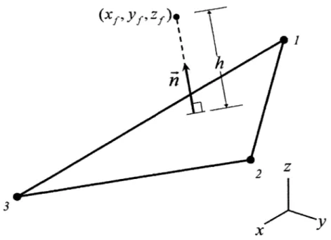
One fundamental assumption when the IIM method is used for interpolating displace-ments and/or rotations is that the CFD data points are all assumed to lie on the planar surface of the CSD elements. Of course, the CFD points are not assumed to coincide in any way with the CSD nodes, but to use the 2D formulation of IIM, these CFD points must be assumed to lie on the elements. However, in most aeroelastic applications, the CFD points rarely lie on the planar surface of the CSD elements mainly because the CFD grids are much finer than the CSD meshes. To account for this problem, a method suggested by Brown [16] based on the dynamics of rigid body rotation is used when interpolating displacements and rotations using the IIM method. The method assumes rigid body rotation between the CFD point Pf(X, Y, Z) and an "anchor point" P,(x, y, z) on the CSD element plane. This anchor point is chosen on the CSD element such that it is the closest point from the CFD point to the CSD element. In other words, P, is the orthogonal projection of Pf on the CSD element plane as shown in Figure 2-2. The equations of displacements and rotations at Pf using this method, assuming that the points P1 and P, are connected by a rigid bar,

can be written as,

U(Pf) = u(AS) - (IY - PS) x uO(AS)

U0(Pf) = uO(PS) (2.4)

where U(Pf) and Uo(Pf) are the displacements and rotations of the CFD point, respectively, and u(P8 ) and uo(Ps) are the associated displacements and rotations of the anchor point

(35)

on the CSD element. But the displacements and rotations at any point in a finite element can be written as function of the nodal displacements (ui, vi, wi) and shape functions Ni. Therefore, using similar notations as in Equation 2.2 and Equation 2.3, Equation 2.4 can be rewritten as U(P

{

UO(Pf)={

U V w (Z (y Ox OY

Oz

- wi 0 (z-Z) (Y-y) Z) 0 (X-X) -Y) (X - X) 0

Q~ OX1

II

oyx %Ni

J

where (X, Y, Z) are the coordinates of Pf and (X, Y, Z) are the coordinates of P. In order to find the partial derivatives of Ni

(

, r7) with respect to the global coordinate system x, y, and z, a 2D Jacobian matrix is needed, which is discussed in Appendix A.

If the rotations in the CSD mesh are not given, the above method can still be used correct for the point to be interpolated not lying in the CSD plane. The rotations can approximated by the derivatives of the displacement field. Therefore, Equation 2.5 can written as

U(Pf)

U] V w -Pf 0 (Z-z (y- Y = ZNi(y, ) (z - Z) (Y -0 (x-(X - X) 0 0 0 0 0

zz

zi

1w

y)

X)

ax 0J to be be

I

ui Vi Wi

I

(2.6)

Oxi

Oyi Ozi

I

(2.5) =L

(36)

Once again, to obtain N, and '9Ni from ' and %9N, the Jacobian transformation matrix must be applied, which is discussed in Appendix A.

Interpolating Loads

Although the same shape functions are used to interpolate loads, this interpolation has a slightly different procedure than that used for displacements or rotations. Transforming concentrated loads from a CFD grid to a CSD mesh can be based on the criteriom of conservation of virtual work done by a set of applied loads [1]. Let Ff represent a column matrix of given concentrated loads at a set of points Pf on the CFD grid, the virtual work done by this set of loads is given by

6W

= Ff T6uf (2.7)

where 6uf is a compatible virtual discretized displacement field corresponding to the set of points Pf.

It is possible to define an equivalent set of concentrated loads on a set of points P, on the structural mesh such that the virtual work is the same. This condition will satisfy the conservation of total force and moment about any point on the system. Let F, represent the set of concentrated loads on the set of CSD nodes P that is equivalent to Ff, then

F[

oUs=Fruf

F (2.8)

where 6u, is a compatible virtual discretized displacement field corresponding to the set of points P.

Assume that the displacement field is known to be interpolated between these two sets of points using

us = T uf (2.9)

where T is the transformation matrix relating the two displacement sets. Virtual displace-ment fields must also follow the same transformation to satisfy compatibility, such that

CFD/CSD grid interfacing of three-dimensional surfaces by inverse isoparametric maping

CFD/CSD Grid Interfacing of Three-Dimensional Surfaces

by Inverse Isoparametric Mapping

Pong Kwong Lee

MASTER OF SCIENCE

MASSACHUSETTS INSTITUTE OF TECHNOLOGY

@

SEP

11 2001

CFD/CSD Grid Interfacing of Three-Dimensional Surfaces by Inverse

Isoparametric Mapping

Abstract

Acknowledgments

Contents

List of Figures

AGARD 445

AGARD 445

List of Tables

Chapter 1

Introduction

1.1

Motivation

1.2

Previous Work

1.3

Present Work

1.4

Scope of Thesis

Chapter 2

Mathematical Formulation

2.1

Inverse Isoparametric Mapping Method

1

rq

2

2

Y

3

x

M

L

~3

1W P

((,

((,

((,

((,

((,

ox

z

i~=

ay~~

Ozi

Pf (X,Y,

Z)

projection I

CFD grid points

CSD plane

{

UO(Pf)={

Oz

Q~ OX1

II

J

(

U(Pf)

zz

1w

X)

I

I

I

Oxi

I

6W

F[

oUs=Fruf

_ox

_z

_i~=

_ay~~

_Ozi