HAL Id: hal-01872023
https://hal.archives-ouvertes.fr/hal-01872023
Submitted on 11 Sep 2018HAL is a multi-disciplinary open access archive for the deposit and dissemination of sci-entific research documents, whether they are pub-lished or not. The documents may come from teaching and research institutions in France or abroad, or from public or private research centers.
L’archive ouverte pluridisciplinaire HAL, est destinée au dépôt et à la diffusion de documents scientifiques de niveau recherche, publiés ou non, émanant des établissements d’enseignement et de recherche français ou étrangers, des laboratoires publics ou privés.
The Physical Layer of Low Power Wide Area Networks:
Strategies, Information Theory’s Limit and Existing
Solutions
Yoann Roth, Jean-Baptiste Doré, Laurent Ros, Vincent Berg
To cite this version:
Yoann Roth, Jean-Baptiste Doré, Laurent Ros, Vincent Berg. The Physical Layer of Low Power Wide Area Networks: Strategies, Information Theory’s Limit and Existing Solutions. Advances in Signal Processing: Reviews, Vol. 1, Book Series, 2018. �hal-01872023�
Chapter 7
The Physical Layer of Low Power Wide Area
Networks: Strategies, Information Theory’s
Limit and Existing Solutions
Yoann Roth, Jean-Baptiste Doré, Laurent Ros and Vincent Berg
17.1. Introduction
The Internet-of-Things (IoT) is a trending topic and the focus of many current research works [1]. The general definition of IoT was first suggested by the International Telecommunication Union (ITU) in 2012 [2]. It is defined as a global infrastructure based on existing and evolving communication technologies and interconnecting things. “Things” refer to many possible entities such as sensors or actuators as well as more complex systems such as vehicles or buildings. The existing communication technologies mentioned in the definition refer to legacy networks (Long Term Evolution, WiFi, Bluetooth, etc.), which are still expected to be used for the IoT. Evolving communication technologies correspond to new networks that must be designed and deployed. Low Power Wide Area Networks (LPWAN) are part of these networks [3, 4], and 10 % of the overall IoT connections are expected to be done through them [5]. LPWAN aims to offer a technical solution for applications that require a long range of communication and a low consumption at the “thing” level, i.e. the device.
LPWAN differs from legacy cellular networks by both the requirements and the possible applications. These networks are commonly characterized by some key features [6]:
• Long range communication; • Low throughput communication; • Low cost devices;
• Long battery life for the devices (up to 10 years).
Yoann Roth
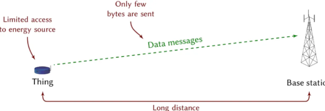
To illustrate the various requirements for the physical layer of LPWAN, a simple schematic of the exchange of messages between the “thing” and the base station is depicted in Fig. 7.1. The long range is featured by a long distance between the “thing” and the base station, which collects the signal and transmits it further in the IoT network. This means that the physical layer must be designed in such a way that even highly attenuated signals can be decoded at the base station. In a later section, we will see how achieving long range is related to the notion of sensitivity, and define this concept. Usually, a low throughput is considered for LPWAN applications, i.e. only a few bytes are transmitted by the device. However, we will see that this requirement can also be interpreted as a consequence of the necessity for a long range. Devices are expected to be low cost with the capability to offer only few applications (unlike a smartphone, offering hundreds of possible applications). Complexity of the operation realized by the devices must be either efficiently done or reduced to a minimum. Low cost operating units could thus be considered. This problematic is closely related to the low power constraint, as low computational capacity may lead to a lower energy consumption. The device must be energy efficient, since it is assumed to have no access to an energy source. A long battery life is thus required and energy must be saved in any possible way. In the transmission chain, the most consuming element is the Power Amplifier (PA) [7]. This component is in charge of amplifying the signal to be transmitted through the air. For LPWAN, the modulation should therefore be chosen to minimize the consumption of the PA, as this would dramatically reduce the consumption of the device and save battery life.
Fig. 7.1. Illustration of the exchange of messages in the context of LPWAN.
This chapter is dedicated to the study of the physical layer of LPWANs. It is divided into three sections, each one addressing a different problematic. The first one concerns the analysis of the constraints imposed on the physical layer of LPWAN due to its various features. The second section is dedicated to the identification of the strategies that allow for long range transmission. Several techniques are reviewed and compared to the information theory’s limit of the channel capacity, which gives insight into achievable gains. Finally, the last section is a review of the existing LPWAN solutions, including a detailed description of the principle of each technology and a comparison of the techniques.
7.2. Constraints of the Physical Layer
The various features of LPWAN imposes some constraints on the physical layer. In this section, we will see how these constraints are related to two concepts, namely constant envelope modulations and the sensitivity.
7.2.1. Power Amplifier and Constant Envelope Modulations
The PA is one of the last elements of the transmission chain. It converts the low-level signal to a high-power signal to be transmitted through the transmitter antenna [8]. This critical component turns out to be a high energy consumer, and selecting an efficient PA is a major concern when designing a Radio Frequency (RF) system [7]. When considering LPWAN, the PA needs to be highly energy efficient and low cost, thus ensuring a longer battery life for the device and reducing its cost. The efficiency of a PA is closely related to the variations of the envelope of the amplified signal. In Fig. 7.2, the typical output power of a PA is depicted versus its input power. The ideal amplifier (in dashed) performs linear amplification. However, in common amplifiers (plain curve, in red), the output power is limited to the saturation level denoted 𝑃𝑃sat, and the amplification stops being linear from a certain input power value. Non-linearities introduced by the amplification induce distorsions of the output signal, such as apparition of out-of-band harmonics. In order to avoid these effects, the input power is regulated and kept outside of the non-linear region of the amplifier. The 1 dB compression point corresponds to the value of input power for which the output power is reduced of 1 dB compared to the ideal amplifier response. This value is often chosen as the maximum acceptable input power, i.e. as the beginning of the non-linear region of the amplifier.
Fig. 7.2. Output power versus input power for a typical power amplifier.
The envelope of the signal to be amplified often experiences variations. These variations are commonly characterized by the Peak-to-Average Power Ratio, defined as
PAPR(𝐵𝐵𝒍𝒍) =
max𝑘𝑘 �|𝑥𝑥(𝑘𝑘)|2�
𝐸𝐸[|𝐱𝐱|2] ,
where 𝐵𝐵𝑙𝑙 is the block index corresponding to the time interval, 𝐱𝐱 is the signal to be amplified and 𝑥𝑥(𝑘𝑘) its elements with 𝑘𝑘 ∈ {0, … , 𝑁𝑁block− 1} where 𝑁𝑁block is the size of the considered block 𝐵𝐵𝑙𝑙. The PAPR is a statistical measure, and it is often the Complementary Cumulative Distribution Function (CCDF) of the PAPR which is evaluated. It describes how the values of the PAPR are distributed.
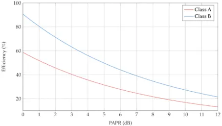
Since the PAPR describes the variation of the envelope, it also indicates how to drive the input of the PA. In order to avoid the non-linear region, a back-off from the compression point is considered for the input power 𝑃𝑃in, as represented in Fig. 7.2. This back-off is selected depending on the distribution of the PAPR. Selecting a specific back-off will ensure the PA to reach the non-linear region for only a given probability, which is usually chosen as a low value. The consequence of selecting a large back-off (or equally, that high values for the PAPR are more likely), is that the average level of output power is lowered. The efficiency of the PA can be shown to be dependent on the level of output power [9]. For class A and B amplifiers, the theoretical efficiency versus the level of PAPR is depicted in Fig. 7.3. Dealing with a signal that exhibits a high PAPR will then result in a poor efficiency for the PA, and consequently a high consumption. On the opposite, dealing with a signal that exhibits no variation will allow the PA to be driven directly at the compression point, thus ensuring the maximum possible efficiency. These signals are called constant envelope signals and have a PAPR equal to 0 dB.
Fig. 7.3. Theoretical efficiency of class A and class B amplifiers versus the PAPR.
A constant envelope modulation is a modulation which generates a constant envelope signal. For LPWAN, these types of modulation are of prime importance as they allow to increase the efficiency of the PA and to reduce the energy consumption. Used at the device level, they ensure a longer battery life. We will see that most of the existing solutions employ constant envelope modulations.
7.2.2. Achieving Long Range
As mentioned previously, one of the requirements for the physical layer of LPWAN is to be able to communicate at long range. The range of the communication can be defined as the distance 𝑑𝑑 for which the Quality of Service (QoS) is reached. This Qos is often expressed in terms of Bit Error Rate (BER) or Packet Error Rate (PER). In order to express this distance with the other parameters of the system, we consider Line-of-Sight (LOS) and free path loss for the transmission. This simplified model will allow us to clearly identify the strategies employed by LPWAN solutions. Using the Friis equation [10], the square of the distance 𝑑𝑑 is expressed
𝒅𝒅𝟐𝟐=𝑷𝑷𝒕𝒕𝑮𝑮𝒕𝒕𝑮𝑮𝒓𝒓 𝑷𝑷𝒓𝒓 � 𝛌𝛌 𝟒𝟒𝝅𝝅� 𝟐𝟐 , (7.1)
where 𝑃𝑃𝑡𝑡 (resp. 𝑃𝑃𝑟𝑟) is the power at the transmitter side (resp. the receiver side), 𝐺𝐺𝑡𝑡 (resp. 𝐺𝐺𝑟𝑟) is the antenna gain of the transmitter (resp. the receiver), and λ is the wavelength of
the transmitted signal. In this equation, several of the quantities could vary for the distance to increase. However, most of the quantities are subject to regulations, either for economical or sanitary reasons. Namely the transmitted power 𝑃𝑃𝑡𝑡, the antenna gains or the wavelength λ (inversely proportional to the carrier frequency) are regulated, for example by the Federal Communications Commission (FCC) for the United States of America [11]10/16/2017 9:02:00 PM. All these quantities can be considered as constants. The square of the distance becomes proportional to the inverse of the received power 𝑃𝑃𝑟𝑟. As the range was defined for a given QoS, the value 𝑃𝑃𝑟𝑟 is the level of received power required to obtain that QoS. That quantity is often referred to as the sensitivity of the receiver, and represents the only available degree of freedom to reach long range. By reducing the sensivity level, long range can be achieved.
7.2.3. Sensitivity of the Receiver
The sensitivity of the receiver was introduced previously as the level of received power required to obtain the specific QoS. This quantity is a power and can be expressed with
𝑃𝑃𝑟𝑟 = 𝐸𝐸𝑏𝑏,𝑟𝑟𝑟𝑟𝑟𝑟𝑅𝑅, (7.2)
where 𝐸𝐸𝑏𝑏,𝑟𝑟𝑟𝑟𝑟𝑟 is the average energy of one bit required for the QoS, expressed in Watt.s, and 𝑅𝑅 is the binary rate, expressed in bit/s. The value 𝐸𝐸𝑏𝑏,𝑟𝑟𝑟𝑟𝑟𝑟 is intrinsic to the technology selected. This genuinely simple equation gives the principle behind most of the technologies for LPWAN, which is to reduce the data rate 𝑅𝑅. Indeed, reducing the data rate reduces the sensitivity, and thus increases the range of the communication.
In order to illustrate this effect, we propose a comparison of the performance, under Additive White Gaussian Noise (AWGN), of a same technique, the Binary Phase Shift Keying (BPSK), with various rates. Rates from 100 bps to 10 kbps are selected. The PER for a packet of size 128 bytes is computed for various values of received power, expressed in dBm. The result is depicted in Fig. 7.4. The sensitivity of each technique is evaluated
by selecting a specific QoS and its associated received power. For example, if we choose a QoS corresponding to a PER of 10−2, the sensitivities of the rates 100 bps, 1 kbps and 10 kbps are equal to -144.5 dBm, -134.5 dBm and -124.5 dBm, respectively. Using (7.1) with all parameters constant except the distance and the receiver’s power (i.e. the sensitivity), the gain in distance between two techniques can be expressed with
𝑑𝑑1
𝑑𝑑2= �
𝑃𝑃𝑟𝑟𝑟𝑟𝑟𝑟,2
𝑃𝑃𝑟𝑟𝑟𝑟𝑟𝑟,1, (7.3)
where 𝑑𝑑1 (resp. 𝑑𝑑2) is the distance between the transmitter and the receiver of the first (resp. the second) technique, and 𝑃𝑃𝑟𝑟𝑟𝑟𝑟𝑟,1 (resp. 𝑃𝑃𝑟𝑟𝑟𝑟𝑟𝑟,2) the sensitivity of the first (resp. the second) technique, expressed in linear. The gain of 10 dB in sensitivity achieved by considering a data rate of 100 bps instead of a data rate of 1 kbps can thus be interpreted as a gain equal to 3.2 in the range of the transmission (for a constant transmit power). Simply by reducing the data rate, a gain in range was achieved.
Fig. 7.4. PER performance under AWGN of BPSK with various data rates, versus
the received power.
The reduction of the data rate can be done through several strategies. Before presenting these strategies, another expression of the sensitivity is formulated.
The receiver, as any electronic device, is subject to thermal noise. This electronic noise is due to the thermal agitation of the electrons, and is proportional to the ambient temperature. The noise power can be expressed
𝑃𝑃𝑛𝑛= 𝑁𝑁0𝐵𝐵,
where
𝑁𝑁0= 𝑘𝑘𝐵𝐵𝑇𝑇,
with 𝑘𝑘𝐵𝐵 the Boltzmann’s constant (equal to 1.3806 ⋅ 10−23 Joules/K) and 𝑇𝑇 the temperature, in Kelvins. 𝐵𝐵 is the bandwidth of the signal, in Hertz. 𝑃𝑃𝑛𝑛 is expressed in
Watts, or Joules/s. The quantity 𝑁𝑁0 is commonly referred to as the noise power spectral density. In order to characterize the noise versus the signal power, we define the Signal-to-Noise Ratio (SNR) as
SNR =𝑃𝑃𝑃𝑃
𝑛𝑛=
𝑃𝑃
𝑁𝑁0𝐵𝐵. (7.4)
Typical receivers also present some imperfections that affect the SNR. In order to characterize the loss compared to an ideal receiver, the noise factor 𝐹𝐹 is introduced, with 𝐹𝐹 ≥ 1 [12]. When the receiver is considered ideal, the noise factor is taken to equal 1. A new expression of the sensitivity, including the noise factor of the receiver and expressed in W, can be derived as
𝑃𝑃req= SNRreq⋅ 𝑁𝑁0⋅ 𝐵𝐵 ⋅ 𝐹𝐹,
where SNRreq is the ratio between the sensitivity as defined in Eq. (7.2) and the noise power. As we usually deal with small values for 𝑃𝑃req, it is common to express the power in dBm, using the conversion
�𝑃𝑃req� dBm = 10log10�10𝑃𝑃req−3�,
where the division by 10−3 stands for the fact that we consider the ratio of the power (in Watt) over 1 mW. More generally, we choose to represent any ratio in dB, or 10 times the base 10 logarithm of the power ratio. The sensitivity in dBm is thus given by
�𝑃𝑃req� dBm= SNR dBreq+ 10log10(𝐵𝐵) + 10log10(𝑁𝑁0⋅ 103) + 10log10(𝐹𝐹).
The quantity 10log10(𝑁𝑁0⋅ 103) is often taken equal to −174 dBm, which is its value for 𝑇𝑇 ≃ 288 K (≃ 15 °C). The noise factor expressed in dB is called the noise figure 𝑁𝑁𝐹𝐹.
Unless stated otherwise, we consider that the front end of the receiver does not add any additional noise, and thus has a noise figure 𝑁𝑁𝐹𝐹 = 0 dB. Typical noise figures can range from 1 to 15 dB when not considering deep space applications [12]. With these simplifications, the expression of the sensitivity becomes
�𝑃𝑃req� dBm = SNRreq dB + 10log10(𝐵𝐵) − 174. (7.5)
7.3. Strategies
When simply expressing the sensitivity from the expression of the signal power, it appeared that the most obvious solution to increase the range of the communication is to reduce the data rate. In the new expression of the sensitivity, given in Eq. (7.5), the same solution appears implicitly. What appears clearly is the two main possible strategies to reduce the sensitivity: reducing the value of 𝐵𝐵, the bandwidth, and reducing the value of
SNR dBreq, the required SNR for the QoS. This second strategy can allow a reduction of the
level of sensitivity while maintaining a constant data rate. In this section, we will review the different strategies and their implications. Performance of examples of technique following the presented strategies will also be presented.
7.3.1. Reduce the Bandwidth
The first strategy to reduce the sensitivity is to reduce the bandwidth of the signal. In the example of Fig. 7.4, this was that strategy that was considered. For a given technique, reducing the bandwidth implies a reduction of the data rate, and consequently a reduction of the level of sensitivity. Following this strategy implies to deal with narrow band signals. While the term “narrow” is somehow relative (e.g. 10 kHz is narrow compared to 10 MHz), it is common for LPWAN to consider Ultra Narrow Band (UNB) signals, for which the bandwidth is less than 1 kHz [13]. By considering such small bandwidths, very low levels of sensitivity can be obtained. The use of UNB signals allows for very simple transceiver to be used and lowers the cost of the device. However, due to their small bandwidth, UNB signals are very sensitive to frequency drifts (for example a Doppler shift due to mobility or a carrier frequency offset due to a low-quality oscillator). They impact negatively both the detection and the demodulation of the UNB signal. In the case of multi-user transmission, frequency drifts also lead to a larger number of collisions [13]. While UNB signaling is a clearly identified strategy for LPWAN, this technique alone does not offer flexibility in the design of the physical layer. Any technique can be selected and associated to a UNB signal. For the following sections, we focus on the second strategy, which offers more flexibility regarding the physical layer’s design.
7.3.2. Reduce the Required Signal-to-Noise Ratio
The second strategy is to reduce the SNR. The expression presented previously can be modified to explicitly show different ways to reduce the SNR. Associating Eq. (7.2) with Eq. (7.4), the SNR is expressed
SNR𝑟𝑟𝑟𝑟𝑟𝑟=𝑃𝑃𝑁𝑁𝑟𝑟𝑟𝑟𝑟𝑟0𝐵𝐵 = 𝐸𝐸𝑏𝑏,𝑟𝑟𝑟𝑟𝑟𝑟𝑁𝑁0𝐵𝐵𝑅𝑅= �𝑁𝑁𝐸𝐸𝑏𝑏0�
𝑟𝑟𝑟𝑟𝑟𝑟× 𝜂𝜂. (7.6)
where
𝜂𝜂 =𝑅𝑅𝐵𝐵,
is the spectral efficiency, expressed in bits/s/Hz. This expression explicits the three main methods used to reduce the level of SNR, which may or may not lead to a reduction of the data rate.
7.3.2.1. Reduce the Spectral Efficiency
The first method is to reduce the spectral efficiency η only. This is commonly realized through the use of a repetition factor, sometimes referred to as Spreading Factor (SF). This trivial technique repeats the information a total of λ times at the transmitter side. The receiver is able to recombine (using Maximal-Ratio Combining) the repetitions and to achieve a processing gain in SNR. This gain, expressed in dB, is equal to 10log10(λ). However, the technique does not allow for a gain in 𝐸𝐸𝑏𝑏/𝑁𝑁0. If we consider a primary technique with a given required SNR noted 𝑆𝑆𝑁𝑁𝑅𝑅1, the gain in SNR achieved when repeating by a factor λ can be expressed
𝑆𝑆𝑁𝑁𝑅𝑅λ=𝑆𝑆𝑁𝑁𝑅𝑅λ1.
Using (7.6), the expression becomes �𝐸𝐸𝑏𝑏 𝑁𝑁0�λ𝜂𝜂λ= 1 λ� 𝐸𝐸𝑏𝑏 𝑁𝑁0�1𝜂𝜂1,
and since the use of the repetition divided the spectral efficiency by the factor λ, we have 𝜂𝜂λ=𝜂𝜂λ1, and thus �𝐸𝐸𝑏𝑏 𝑁𝑁0�λ= � 𝐸𝐸𝑏𝑏 𝑁𝑁0�1,
which demonstrates that the level of 𝐸𝐸𝑏𝑏/𝑁𝑁0 remains unmodified by the application of the repetition factor.
When considering a fixed bandwidth B, the level of sensitivity (in dB) is reduced by the same factor 10log10 (λ) and the data rate is reduced by a factor λ. It is thus possible to reach very low levels of sensitivity using the repetition factor, at the expense of a reduced spectral efficiency. This simple technique is widely used, for example in the Direct Sequence Spread Spectrum (DSSS), which is employed in the Coded Division Multiple Access (CDMA) technique [14].
7.3.2.2. Reduce the Spectral Efficiency Along with the Required 𝑬𝑬𝒃𝒃/𝑵𝑵𝟎𝟎
The other method to reduce the level of SNR is to reduce the level of required 𝐸𝐸𝑏𝑏/𝑁𝑁0 along with a reduction of the spectral efficiency. The most common way to reduce both 𝐸𝐸𝑏𝑏/𝑁𝑁0 and the spectral efficiency is to use Forward Error Correction (FEC), also called
channel coding [15]. Principle of FEC is to add redundancy at the transmitter (thus reducing the spectral efficiency), and to use an efficient receiver that will require a smaller level of 𝐸𝐸𝑏𝑏/𝑁𝑁0 to reach the same QoS. Various families of FEC codes exist, and each family offers various ranges of spectral efficiency and required 𝐸𝐸𝑏𝑏/𝑁𝑁0. A powerful FEC
solution is the Turbo Code (TC) [16], which combines the use of two Convolutional Codes (CC) with an iterative receiver. This family allows for high gains in 𝐸𝐸𝑏𝑏/𝑁𝑁0 at the expense of a reasonable reduction of the spectral efficiency. The TC have been extensively studied in the literature and are used in the current generation of cellular networks, the 4G [17]. Another interesting technique which reduces both the spectral efficiency and the level of required 𝐸𝐸𝑏𝑏/𝑁𝑁0 is the use of M-ary orthogonal modulations [18]. When using orthogonal modulation, an alphabet composed of M symbols (or codewords) is considered. Groups of log2𝑀𝑀 bits are then associated to one of the symbols from the alphabet. The alphabet is said to be orthogonal as pairs of distinct symbols have an inner product equal to zero. If we consider orthogonality with complex (versus real) inner product, a symbol is composed of M chips (or samples) where the chip rate is equal to 1/𝑇𝑇𝑐𝑐, with 𝑇𝑇𝑐𝑐 the chip time. The (minimum) bandwidth of the signal is thus equal to 𝐵𝐵 = 1/𝑇𝑇𝑐𝑐 (after frequency carrier translation). The symbol time 𝑇𝑇𝑠𝑠 can be obtained with 𝑇𝑇𝑠𝑠 = 𝑀𝑀𝑇𝑇𝑐𝑐, and the symbol rate is equal to 1/𝑇𝑇𝑠𝑠. The binary rate is given by 𝑅𝑅 = 𝐵𝐵log2( 𝑀𝑀)/𝑀𝑀 for complex inner product (and would be twice this value for real inner product).
Examples of orthogonal modulation include Pulse Position Modulation (PPM) or Frequency Shift Keying (FSK) modulation. In Fig. 7.5, the binary words association, sampled time symbols (each composed of 4 chips), baseband waveforms and shaped spectrums of the elements of the 4-FSK modulation alphabet are depicted. This modulation is said to be localized in frequency as each symbol is localized around a specific frequency. The minimum subcarrier spacing is 1/Ts (resp. 1/2Ts) for an orthogonality with complex inner product (resp. real inner product). Orthogonal modulations are said to be energy efficient as the level of required 𝐸𝐸𝑏𝑏/𝑁𝑁0 for a specific QoS is reduced when the size of the alphabet M increases. However, the spectral efficiency is also reduced with the size of M. It is expressed (and would be twice if orthogonality was ensured only for real inner product instead of complex one):
𝜂𝜂 = log2𝑀𝑀
𝑀𝑀 .
Fig. 7.5. Binary words association, sampled time symbols, baseband waveform and shaped
Since these modulations are spectrally inefficient, they are not often considered for high rate applications. Instead, linear modulations (such as Phase Shift Keying (PSK) or Quadrature Amplitude Modulation (QAM)) are used, as they offer an increased spectral efficiency with an increasing size of alphabet M. One of the drawbacks of linear modulations is that the required level of 𝐸𝐸𝑏𝑏/𝑁𝑁0 increases as well with the size of alphabet, making these modulations inefficient regarding the energy. For LPWAN, orthogonal modulations are preferred as they allow to reach for low levels of sensitivity through the reduction of both the spectral efficiency and the level of required 𝐸𝐸𝑏𝑏/𝑁𝑁0.
7.3.2.3. Reduce the Level of Required 𝑬𝑬𝒃𝒃/𝑵𝑵𝟎𝟎
Eq. (7.6) indicates that it is possible to reduce the SNR by reducing the level of 𝐸𝐸𝑏𝑏/𝑁𝑁0 only, i.e. with a constant data rate or spectral efficiency. This can be done by selecting a different modulation technique (while maintaining the spectral efficiency constant) or by choosing a different FEC. For example, using a rate 1/3 TC instead of a rate 1/3 CC may lead (depending on the information block size selected) to a reduction of the required 𝐸𝐸𝑏𝑏/𝑁𝑁0 for a given data rate. More generally, it is possible to reduce the level of required
𝐸𝐸𝑏𝑏/𝑁𝑁0 simply by optimizing the receiver.
In order to express more clearly the impact of the level of required 𝐸𝐸𝑏𝑏/𝑁𝑁0 on the level of sensitivity, (7.5) is expressed using (7.6) and the definition of the spectral efficiency. It gives
�𝑃𝑃req� dBm = �𝐸𝐸𝑁𝑁𝑏𝑏0� req dB
+ 10log10(𝑅𝑅) − 174. (7.7)
This new expression of the sensitivity distinguishes differently the techniques: those that reduce the data rate R only (for example, UNB signalling or repetition), those that reduce the level of 𝐸𝐸𝑏𝑏/𝑁𝑁0 only (for example, the use of a more efficient FEC), and those that reduce both, such as orthogonal modulation. Overall, all these techniques lead to a reduction of the sensitivity, but they may do it in a more or less efficient way.
7.3.3. Comparison to the Information Theory’s Limit
In order to assess the efficiency of the different techniques, their performance (in both spectral efficiency and level of 𝐸𝐸𝑏𝑏/𝑁𝑁0) is compared with the information theory’s limit of the transmission medium. This limit was defined by Claude Shannon in 1948 [19] and it commonly referred to as the channel capacity. The capacity corresponds to the maximum achievable data rate under AWGN for an arbitrarily small level of error. It is expressed in bits/s and denoted C, with
𝐶𝐶 = 𝐵𝐵log2(1 + SNR).
By dividing the capacity by the bandwidth B, we obtain the maximum achievable spectral efficiency 𝜂𝜂max expressed by
𝜂𝜂max = log2(1 + SNR).
With the definition of the SNR given in Eq. (7.6), the maximum achievable spectral efficiency can be expressed with
𝜂𝜂max= log2�1 +𝑁𝑁𝐸𝐸𝑏𝑏0⋅ 𝜂𝜂max�,
or alternatively, the limit can be expressed as the minimum achievable level of 𝐸𝐸𝑏𝑏/𝑁𝑁0. This value corresponds somehow to the maximum achievable energy efficiency of the system for a given spectral efficiency and an arbitrarily small level of error. This quantity is expressed
�𝐸𝐸𝑏𝑏
𝑁𝑁0�min=
2𝜂𝜂−1
𝜂𝜂 . (7.8)
(𝐸𝐸𝑏𝑏/𝑁𝑁0)min is thus an increasing function of the spectral efficiency. This means that it is
possible to increase the spectral efficiency as wanted at the expense of an increased level of 𝐸𝐸𝑏𝑏/𝑁𝑁0, i.e. a reduction of the energy efficiency. However, the value (𝐸𝐸𝑏𝑏/𝑁𝑁0)min is bounded when 𝜂𝜂 → 0, with the limit being equal to
�𝐸𝐸𝑏𝑏
𝑁𝑁0�lim= ln 2 ≈ −1.59 dB,
While the (𝐸𝐸𝑏𝑏/𝑁𝑁0)min is the minimum achievable level of 𝐸𝐸𝑏𝑏/𝑁𝑁0 for a given spectral efficiency, (𝐸𝐸𝑏𝑏/𝑁𝑁0)lim is the absolute minimum achievable level of 𝐸𝐸𝑏𝑏/𝑁𝑁0.
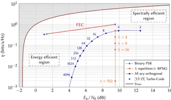
In Fig. 7.6, the maximum achievable spectral efficiency is depicted versus the level of 𝐸𝐸𝑏𝑏/𝑁𝑁0. The operating zone of any reliable communication system must be in the area
under the curve, which is generally divided into two main regions. The first region is the spectrally efficient region. In this area, spectral efficiency is high (> 1) while the 𝐸𝐸𝑏𝑏/𝑁𝑁0 is high as well. This region concerns techniques designed for very high data rates without considering the energy efficiency as a major constraint. The second region, which is the region of interest for LPWAN, is the energy efficient region. For this region, the level of 𝐸𝐸𝑏𝑏/𝑁𝑁0 is low (inducing a high energy efficiency) but so is the spectral efficiency. This
area concerns techniques for which the energy efficiency constraint is very high, while a lower data rate is required, or more bandwidth usage is accepted. From the information theory, the conclusion is that a trade-off between the spectral efficiency and the energy efficiency must always be made.
The figure also depicts the performance of several techniques following the previously presented strategies. For each point, simulations were run to find the level of 𝐸𝐸𝑏𝑏/𝑁𝑁0 required to obtained a QoS equivalent to a BER equal to 10−5. For the repetition factor solution, the BPSK is considered as primary technique. As mentioned previously, the use of a repetition reduces the spectral efficiency but not the level of required 𝐸𝐸𝑏𝑏/𝑁𝑁0. This appears clearly on the figure. A consequence is that the technique cannot approach the channel limit, there will always be a gap in 𝐸𝐸𝑏𝑏/𝑁𝑁0. This means that the channel resource is not used in the most efficient way.
On the other hand, the use of orthogonal modulations allows to reduce both the spectral efficiency and the level of required 𝐸𝐸𝑏𝑏/𝑁𝑁0 by increasing the size of alphabet. The orthogonal modulation gets closer to the channel capacity as the size of alphabet increases, eventually reaching the capacity for an infinite size of alphabet [18]. Unfortunately, this implies a spectral efficiency tending towards 0, which is not conceivable for practical solutions.
Fig. 7.6. The maximum achievable spectral efficiency along with performance of various
techniques following the strategies presented
In the figure, the performance of the rate-1/3 [13 15] TC for a block size of 1000 bits and 10 decoding iterations is depicted. Associated with BPSK modulation, the scheme requires a level of 𝐸𝐸𝑏𝑏/𝑁𝑁0 of 1 dB to reach a BER of 10−5. Compared to the uncoded modulation, this represents a gain of 8.6 dB, which is considerable. Using this FEC, the gap to the minimum achievable spectral efficiency is only equal to 2 dB.
In the representation, we considered a normalization by the bandwidth. UNB signaling is achieved by considering very small bandwidths. As a consequence, narrow band solutions will appear very far from the capacity, even though it can be used to achieve low levels of sensitivity. One could for example imagine a solution using the BPSK modulation associated with UNB signaling. A simple physical layer is used, with performance approximately 9 dB from the capacity. Nonetheless, the choice of UNB signaling will lead to very low levels of sensitivity.
7.4. Existing Solutions
In the previous section, both the constraints on the physical layer and the strategies to achieve long range transmission were presented. In this section, we present five different solutions which rely on the various possible strategies: two proprietary solutions, two standards, and an academic solution.
7.4.1. Proprietary Solutions
Both proprietary solutions presented here are industrial solutions. Only few technical details are available and most of the documentation comes from marketing information. The European Telecommunications Standards Institute (ETSI) nonetheless set-up an Industry Specification Group within TG28 for low throughput networks [20], and some backward engineering of the LoRa physical layer has been performed [21].
7.4.1.1. Sigfox
Sigfox is a French company, created in 2010 and dedicated to LPWAN [22]. The company widely advertised that its technology relies on narrow band signaling. As presented previously, reducing the data rate 𝑅𝑅 = 𝜂𝜂𝐵𝐵 lowers the sensitivity level, and this can be done by reducing either the spectral efficiency of the technique or the bandwidth. Narrow band signaling follows this second approach. A modulation with a relatively high spectral efficiency is used (without any channel coding), functioning at a high 𝐸𝐸𝑏𝑏/𝑁𝑁0, but the bandwidth 𝐵𝐵 is low enough to ensure a satisfying sensitivity level.
Documentation suggests a bandwidth of 100 Hz and DBPSK modulation. This modulation is a memory modulation and the information is in the phase shifts. While using probabilistic decoding, the 𝐸𝐸𝑏𝑏/𝑁𝑁0 required to reach a BER of 10−5 is equal to 9.9 dB. The spectral efficiency is equal to 1 bits/s/Hz. According to Eq. (7.5), with a bandwidth of 100 Hz, the sensitivity is equal to 𝑃𝑃req= −143.7 dBm (without considering the noise
factor of the receiver). 7.4.1.2. LoRa
The LoRa Alliance [23] is an association of companies that collaborate to offer a LWPAN connectivity solution. The physical layer is based on a technology patented by the former company Cycleo and acquired by Semtech since. The original patent [24] describes a technology based on the emission of orthogonal sequences, chosen as chirps, hence the denomination Chirp Spread Spectrum (CSS). The use of chirp signals for communication has been explored before [25], and can be considered as an orthogonal modulation depending of the choice of the chirp sequence. The Zadoff-Chu sequences [26] are orthogonal as the circular autocorrelation of the sequence is zero for all nonzero delays. With a sequence of size 𝑀𝑀, a total of 𝑀𝑀 delayed (or circularly shifted) sequences can be constructed, giving an alphabet of size 𝑀𝑀 where each sequence is orthogonal to another thanks to the autocorrelation property. Alternatively, the process of chirp modulation can
be seen as a form of FSK modulation (i.e. an alphabet of pure frequencies), and then multiplying the complex symbols by the base chirp. Spectrally, this spreads the power over all the carriers instead of exciting only one frequency. The Zadoff-Chu sequence is a Constant Amplitude Zero Auto-Correlation (CAZAC) sequence, and has interesting properties such as constant envelope.
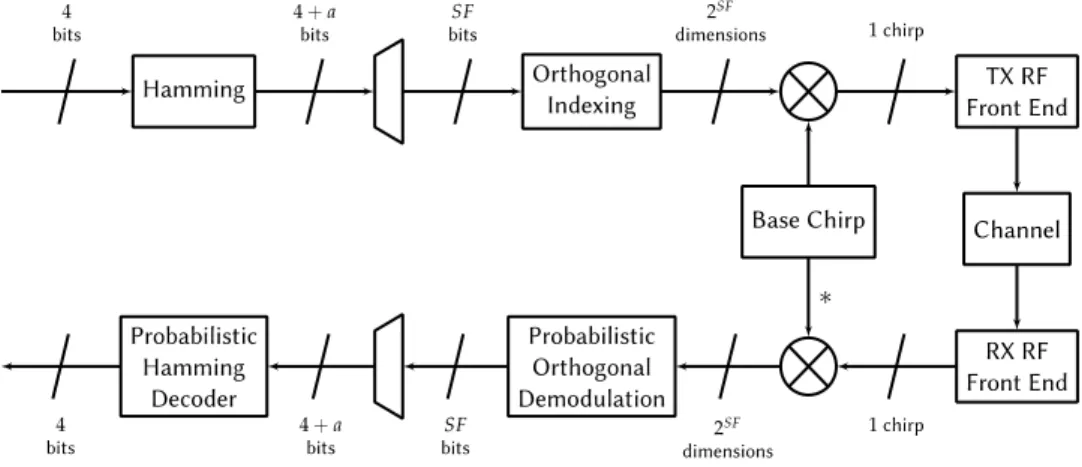
The transmitter and receiver sides of the LoRa modulation are given in Fig. 7.7. While the transmitter is described in the patent [24], we chose the RX side that performs the dual operations of the TX, with ML detection and decoding, as suggested by their technical document [27]. The FEC used is the Hamming code where 𝑎𝑎 parity bits are computed, with 𝑎𝑎 ∈ {1, 2, 3, 4}. The case 𝑎𝑎 = 3 corresponds to the regular Hamming code, while 𝑎𝑎 = 4 is the extended version. The parity bits can also be punctured, i.e.not sent, giving lower values for 𝑎𝑎. After encoding, bits are grouped into words of size 𝑆𝑆𝐹𝐹 (which stands for Spreading Factor (SF), even if it does not match the usual definition of the SF principle. With our notations, SF is equivalent to log2𝑀𝑀 , with M the size of the orthogonal modulation). Each group of bits is associated to one of the 2𝑆𝑆𝐹𝐹 orthogonal dimensions, and the result is multiplied by the base chirps in order to spread the signal on all frequencies.
Fig. 7.7. The LoRa CSSS transmitter and receiver.
At the receiver side, the signal is despreaded by multiplying it with the conjugate of the base chirp. After this step, a classic orthogonal demodulation can be performed, in a coherent or non-coherent way. Each codewords of length 4 + 𝑎𝑎 is then decoded, and the information bits are retrieved. The global spectral efficiency of the scheme is given by
𝜂𝜂 =4+𝑎𝑎4 2𝑆𝑆𝐹𝐹𝑆𝑆𝑆𝑆,
which is coherent with the use of an orthogonal modulation and the rate of the scheme. The LoRa specifications indicate values of 𝑆𝑆𝐹𝐹 from 6 to 12, and a signal bandwidth 𝐵𝐵 = 125 kHz, 250 kHz or 500 kHz.
7.4.2. Standardized Technologies
In telecommunications, standards are defined in order to allow for various systems and operators to coexist. Without some level of standardization, communication between devices would be impossible. The proprietary solutions respect the regulations concerning bandwidth and duty cycles, but need to transmit in the unlicensed frequency bands. These bands are used by numerous applications, thus interference with other users may be high. One of the benefits of using standardized solutions is the possible use of licensed bands, where interference level is contained.
While the technology used by proprietary solutions is kept secret to ensure the monopoly of the inventor company for this very technology, standards are open access and simply define rules to follow for the design of the communication system. Anybody can then create its own system, compliant with the standard, but using their own algorithms for signal detection, demodulation and decoding. In this section, the definition of the rules for the physical layer of two standards are reviewed.
7.4.2.1. 802.15.4k
The 802.15.4k is a standard for local and metropolitan area networks, and is part of the Low-Rate Wireless Personal Area Networks (LR-WPAN) [28]. It aims at low energy critical infrastructure monitoring networks. This standard supports three physical layer modes: Direct Sequence Spread Spectrum (DSSS) with DBPSK or Offset-QPSK, or FSK. DSSS with DBPSK modulation is adapted to more constrained situations, and will be presented here. Standard specifications allow the use of a value 𝑆𝑆𝐹𝐹 from 16 to 32768. Block diagrams for transmitter and receiver are given in Fig. 7.8. The transmitter is composed of a FEC block, defined to be the convolutional code of rate 1/2, with generator polynomials [171 133] and constraint length 𝐾𝐾 = 7. After encoding, interleaving is done to ensure diversity at the reception side. The data is modulated using DBPSK and is “repeated” by the use of a binary direct sequence of size 𝑆𝑆𝐹𝐹. The spectral efficiency of the physical layer is
𝜂𝜂 =2𝑆𝑆𝐹𝐹1 .
The receiver executes the reverse operations of the transmitter side. After dispreading the signal (executing the mean weighted by the elements of the binary direct sequence), we use a soft DBPSK decoder. Given how data was interleaved at the transmitter side, the deinterleaving operation is applied before the Soft Viterbi decoder, designed to retrieve the information bits.
While the standard has been considered as a LPWA solution [29], the Random Phase Multiple Access (RPMA) technique, developed by the US company Ingenu [30], is allegedly based on the 802.15.4k standard, i.e. its physical layer is compliant with the standard. It uses the DSSS technique, and their specific access technique is described by the patent [31]. Regarding the physical layer, we will consider the exact same elements as the 802.15.4k standard, except the possible values for the SF, ranging from 64 to 8192. 7.4.2.2. Narrow-Band IoT
The 3GPP consortium recently issued a standard for the NB-IoT [32]. This standard is actually a new release of the LTE standard [33], and includes three modes for IoT applications. Since it is an evolution of the LTE, it includes other elements of this standard, such as its channel coding procedure [17]. Some industrial group research teams also unveiled more about the NB-IoT standard, such as Nokia [34] and Ericsson [35]. They have two main modes: the uplink (UL) and downlink (DL) modes.
For the UL mode, the modulation can be chosen between BPSK and QPSK, and the FEC used is the [13 15] TC from the LTE standard [17]. The parity bits of the TC can be punctured, giving two possible rates for the channel code: 1/3 and 1/2 (when punctured). The message can be repeated up to 128 times, giving a processing gain at the receiver side.
For the DL mode, i.e. the connection from the base-station to the device, data is modulated using QPSK. The channel code used is a Tail Biting Convolutional Code (TBCC), with generator polynomials [133 171 165], giving a rate 1/3. The use of TBCC allows the receiver (the device) to use a low complexity Soft Viterbi decoder, and the tail biting property avoids the needs to send extra bits to close the trellis. A repetition up to 512 can also be applied.
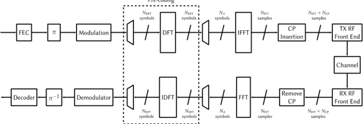
As part of the LTE standard, the data must be modulated using Orthogonal Frequency Division Multiplexing (OFDM) signaling. For the DL, classic OFDM is assumed, while for the UL, both Single Carrier Frequency Division Multiple Access (SC-FDMA) and single tone transmission are considered. Compared to OFDM, both SC-FDMA and single tone offer a lower PAPR [36], which is interesting at the device level as it lowers the energy consumption of the PA.
The architecture of an OFDM/SC-FDMA transceiver is given in Fig. 7.9. Modulated symbols are grouped into blocks of size 𝑁𝑁DFT, and a Discrete Fourier Transform (DFT) of the same size is applied on each group. The symbols are then mapped to 𝑁𝑁𝐴𝐴 carriers, and an Inverse Fast Fourier Transform (IFFT) of size 𝑁𝑁FFT is applied. The mapping of
the symbols is done in the frequency domain and the IFFT generates a signal in the time domain. After this step, a Cyclic Prefix (CP) is inserted, i.e. the last 𝑁𝑁CP samples of a time symbol (which contains 𝑁𝑁FFT samples) are added at the beginning of the symbol, giving a symbol of size 𝑁𝑁FFT+ 𝑁𝑁CP. At the receiving side, after removing the CP, a Fast Fourier Transform (FFT) is applied to recover the mapped symbols from the transmitter. The Inverse Discrete Fourier Transform (IDFT) is then applied to the blocks sent in the first place, in order to recover the modulated symbols. SC-FDMA is a multiplexing technique, as several symbols are transmitted at different frequencies during the same time symbol. The DFT step can be seen as a type of pre-coding, and is omitted when OFDM signaling is considered.
Fig. 7.9. The OFDM/SC-FDMA transmitter and receiver.
The value of 𝑁𝑁𝐴𝐴 is usually equal to 𝑁𝑁DFT, equal to 12, 6 or 3. With the carrier spacing in being 15 kHz, the bandwidth of 12 carriers is equal to 180 kHz. When only a single tone is used, the bandwidth can be chosen equal to 15 kHz or 3.75 kHz. The spectral efficiency of the scheme is given by
𝜂𝜂 = 𝑅𝑅𝑐𝑐⋅𝜂𝜂mod𝑆𝑆𝐹𝐹 ,
where 𝑆𝑆𝐹𝐹 is the repetition factor, 𝑅𝑅𝑐𝑐 the coding rate and 𝜂𝜂mod the spectral efficiency of the modulation used.
7.4.3. Turbo-FSK
The Turbo-FSK is a low spectral efficiency scheme dedicated to LPWAN that we proposed in [37], [38]. It is the result of an academic work, which was inspired from a binary FEC, the Turbo Hadamard [39]. The Turbo FSK scheme is based on the combination of orthogonal waveforms with a low complexity convolutional code associated with an iterative receiver. Turbo-FSK can achieve very low levels of 𝐸𝐸𝑏𝑏/𝑁𝑁0 while ensuring a low complexity transmitter and a constant envelope modulation.
7.4.3.1. Transmitter
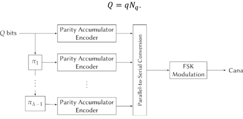
The Turbo-FSK transmitter architecture is depicted in Fig. 7.10. The structure is composed of λ stages, each one encoding an interleaved version of the input bits, with Q the number of input bits. For each stage, the Q bits are segmented into 𝑁𝑁𝑟𝑟 words of q bits, with
𝑄𝑄 = 𝑞𝑞𝑁𝑁𝑟𝑟.
Fig. 7.10. Transmitter of the Turbo-FSK.
The Parity-Accumulator encoder is then applied, as depicted in Fig. 7.11. The parity of each word is computed and accumulated in the memory. The q + 1 bits are then associated one of the codewords from the FSK alphabet. The size of the alphabet is given by 𝑀𝑀 = 2𝑟𝑟+1. The use of the accumulator links every consecutive symbol to the previous
one. The output of each encoder is a set of 𝑁𝑁𝑟𝑟+ 1 FSK codewords (an extra symbol is required to set back the accumulator’s memory to the zero state). A Parallel-to-Serial Conversion is finally realized to send the FSK codewords through the channel. The spectral efficiency of the system is given by
𝜂𝜂 =𝜆𝜆(𝑁𝑁𝑄𝑄
𝑟𝑟+1)𝑀𝑀≈
log2𝑀𝑀−1
𝜆𝜆𝑀𝑀 ,
where the approximation is valid for large sizes of Q. The scheme has three main parameters: the size of alphabet M, the number of stages λ and the block size Q.
7.4.3.2. Receiver
The receiver of the Turbo-FSK system is depicted in Fig. 7.12. The observation of each stage is retrieved by performing a Serial-to-Parallel conversion. Then, for each of the 𝑁𝑁𝑟𝑟+1 codewords, the detector computes the likelihood of the codeword. This can be
performed using the Fast Fourier Transform (FFT) algorithm, and allows the receiver to have an OFDM-like front end. The result of the FFT is a vector of size M, which is the number of possible codewords. The output of the detector is thus a matrix of size (𝑁𝑁𝑟𝑟+ 1) × 𝑀𝑀. This matrix is fed to the decoder, which uses both the observation from
the channel and an a priori information from the other decoder to compute the log-APP of the bits, expressed with
𝐿𝐿(𝑏𝑏|𝒓𝒓) = logPr �Pr �𝑏𝑏 = +1𝑏𝑏 = −1��𝒓𝒓𝒓𝒓��,
where 𝒓𝒓 is the observation. Details about the computation of the log-APP and about how the a priori information is used can be found in [38]. The process is based on the Bahl, Cocke, Jelinek and Rajiv (BCJR) algorithm [40], which is also considered for decoding TCs [41]. The information computed is then passed to the next decoder, and the whole process is repeated for several iterations.
Fig. 7.12. Receiver of the Turbo-FSK.
The Turbo-FSK has been the topic of multiple studies. In [42], the optimization of the scheme was considered, using the well-known EXIT-chart tool [43] for iterative processes. In [44], the implementation of the scheme on off-the-shelf components was studied, and comparison with state of the art techniques was studied in [45]. An extension of the scheme, the Coplanar Turbo-FSK is under investigation [46]. This patented technology improves the flexibility in terms of spectral efficiency of the original Turbo-FSK scheme, thanks to the use of a hybrid alphabet, which holds properties of both linear and orthogonal modulations.
7.4.4. Performance
A total of five different techniques have been presented. To each technique correspond a various number of possible configurations which will lead to different values of spectral efficiencies and required 𝐸𝐸𝑏𝑏/𝑁𝑁0 for a QoS equivalent to a BER of 10−5. Packet sizes of 1000 bits and AWGN are considered. In order to compare the performance of the various schemes, we consider the maximum achievable spectral efficiency as expressed by (7.8). The comparison is depicted in Fig. 7.13. This plot can be divided into three groups, each containing several techniques.
Fig. 7.13. Comparison of the spectral efficiency and required 𝑬𝑬𝒃𝒃/𝑵𝑵𝟎𝟎 (for a BER of 𝟏𝟏𝟎𝟎−𝟓𝟓) of all the configurations and all the scheme, compared to the maximum achievable spectral efficiency
and under AWGN.
The first group contains only the Sigfox technique. Due to its use of UNB signaling, the technology uses a simple physical layer which gives performance rather far from capacity. If the technology can reach low levels of sensitivity, this demonstrates that it does not use the energy resource in the most efficient way.
The second group contains the techniques LoRa, 802.15.4k and RPMA. All these techniques allow for low levels of spectral efficiency. They follow the second strategy, which is to reduce the level of SNR. The solutions related to the 802.15.4k standard only rely on the use of a SF and a convolutional code. The different configurations correspond to different values for the SF, hence the vertical representation of the performance. For LoRa, the use of the orthogonal modulation allows for the level of required 𝐸𝐸𝑏𝑏/𝑁𝑁0 to be reduced with an increasing size of alphabet. However, due to their choice of association of FEC and modulation, the required level of 𝐸𝐸𝑏𝑏/𝑁𝑁0 for the technique remains more than
5 dB from the capacity. By considering the use of a different FEC, the gap to capacity could be reduced.
The third group contains technologies using FEC with iterative receivers. These FEC typically reach lower levels of required 𝐸𝐸𝑏𝑏/𝑁𝑁0. Compared to the second group, a significative gain in 𝐸𝐸𝑏𝑏/𝑁𝑁0 is achieved. The NB-IoT uses the TC [13 15] associated with BPSK, and reaches levels of required 𝐸𝐸𝑏𝑏/𝑁𝑁0 close to 1 dB. However, the value of the block size (1000 bits) reduces the efficiency of the code. The scheme offers a large flexibility in spectral efficiency. When considering low spectral efficiencies, the gap to capacity remains larger than 2.5 dB, but this gap is reduced to 1.5 dB for high spectral efficiencies. The Turbo-FSK relies on the combination of an orthogonal alphabet with a convolutional code, associated with an iterative receiver. In the figure, various combinations of size of alphabet M and number of stages λ were considered. This unconventional association allows for very low levels of required 𝐸𝐸𝑏𝑏/𝑁𝑁0 while achieving low spectral efficiencies. The best combination has been demonstrated to be 𝑀𝑀 = 512 and 𝜆𝜆 = 3 [42] and has a required 𝐸𝐸𝑏𝑏/𝑁𝑁0 only 1.6 dB from the capacity for the considered QoS. Combining this low required 𝐸𝐸𝑏𝑏/𝑁𝑁0 and a low spectral efficiency, the scheme can reach very low levels of sensitivity. However, it should be noted that the scheme is restricted to low spectral efficiencies, lower than 6.25 × 10−2 bits/s/Hz. It is therefore much less flexible than the NB-IoT solution, which can offer spectral efficiencies up to 1 bit/s/Hz.
As mentioned previously, this representation of the performance disregards the value of the bandwidth. It is however possible to compare the range of different techniques by selecting a specific spectral efficiency, and find the technique’s configuration that gives this spectral efficiency. The performance of the 802.15.4k standard, the LoRa technique, the NB-IoT and the Turbo-FSK for a spectral efficiency close to 5.16 × 10−3 bits/s/Hz is depicted in the Fig. 7.14. With these configurations, the 802.15.4k exhibits the poorest performance with a required 𝐸𝐸𝑏𝑏/𝑁𝑁0 equal to 5.7 dB. The LoRa solution performs better with an improvement of the required level of 𝐸𝐸𝑏𝑏/𝑁𝑁0 of 0.9 dB. Here again, iterative solutions perform much better with levels of required 𝐸𝐸𝑏𝑏/𝑁𝑁0 equal to 1 dB and 0 dB for the NB-IoT and the Turbo-FSK, respectively. With these parameters, the Turbo-FSK technique performs 4.6 dB better than the LoRa technique.
Fig. 7.14. Comparison of 4 techniques for a given spectral efficiency, equal to
5.16 × 10−3 bits/s/Hz.
Since the spectral efficiency is set to a constant, the difference in required 𝐸𝐸𝑏𝑏/𝑁𝑁0 of the different techniques compared is similar to the difference in required SNR. We now consider a fixed data rate 𝑅𝑅 = 1.22 kbps for all techniques. This specific data rate corresponds to a bandwidth 𝐵𝐵 = 250 kHz for the LoRa technique, which is an existing configuration according to their specifications. Due to small differences in spectral efficiency between the configurations of the techniques, the bandwidths for the other techniques are slightly different from 250 kHz. In Fig. 7.15, the PER performance under AWGN versus the received power in dBm is depicted for five techniques: the four previous techniques, and the simple BPSK modulation to which was applied a repetition factor of λ = 205. This last technique corresponds to the strategy which consists in reducing the spectral efficiency of a primary technique (in this case, BPSK with a spectral efficiency of 1 bits/s/Hz and a bandwidth of 250 kHz) in order to reduce the data rate (see Section 7.3.2.1 and Fig. 7.6). By selecting a QoS corresponding to a PER of 10−2, the sensitivity for the LoRa technique and the Turbo-FSK are equal to −138.5 dBm and −143.4 dBm, respectively. This 4.9 dB difference in sensitivity can be interpreted in different ways. Using (7.3), the gain in sensitivity of the Turbo-FSK versus the LoRa technique can be interpreted as a gain equal to 1.76 in the range of the transmission (for a constant transmit power). Alternatively, for a constant distance between the transmitter and the receiver, the transmit power in case of Turbo-FSK can be reduced by a factor 3.1.
Fig. 7.15. PER performance under AWGN versus the received power, for the 4 existing
solutions. The data rate is set to 𝑅𝑅 = 1.22 kbps, leading to bandwidths around 250 kHz.
These results demonstrate the capacity of the Turbo-FSK to outperform other systems as well as the potential of turbo coded systems for LPWAN. Additionally, Turbo-FSK employs a constant envelope, which reduces the constraints on the PA (see Section 7.2.1). By considering spectral efficiency practically similar, we ensured a fair comparison of the technique. The difference in sensitivity are observed for a constant data rate and bandwidths of the same order of magnitude.
7.5. Conclusion
This chapter was dedicated to a general presentation of LPWAN. This new type of network is part of the IoT and currently in the process of expansion. The requirements of this network and their implications on the physical layer were presented. The Power Amplifier (PA) is the most consuming element of the transmission chain. However, an adequate choice of modulation can allow for a reduction of the consumption of the PA, along with reduced costs. More specifically, constant envelope modulations are a preferred choice, as they allow the PA to be used up to its compression point. The long-range requirement of LPWAN can be achieved by ensuring a low sensitivity level at the receiver, which is obtained by ensuring a low data rate for the communication. There are several possible strategies to reduce the data rate. For example, Ultra Narrow Band (UNB) signaling or the use of a Spreading Factor can be considered, or potentially a more complex technique such as Forward Error Correction. In order to approach the theoretical limit of the channel while achieving long range, the LPWAN solution should minimize its level of required 𝐸𝐸𝑏𝑏/𝑁𝑁0 for the given QoS. After analyzing these considerations, 5 existing solutions were presented: the Sigfox solution, the LoRa technology, the IEEE 802.15.4k standard, the 3GPP NB-IoT standard and an academic solution, the Turbo-FSK. By comparing the achievable spectral efficiencies and required 𝐸𝐸𝑏𝑏/𝑁𝑁0 for each technique
with various possible configuration, it is clear that turbo coded systems offer a considerably more efficient solution regarding the theoretical bound. Additionally, the flexibility of the NB-IoT solution makes it attractive since a combination of strategies can be considered. For example, selecting the configuration that gives the highest spectral efficiency and a UNB signaling could lead to extremely low levels of sensitivity, with both a constant envelope and a low complexity transmitter. The Turbo-FSK is limited in terms of spectral efficiency but it is a promising academic solution, which additionally employs a constant envelope modulation. An extension, the Coplanar Turbo-FSK, has also been patented and improves the spectral efficiency flexibility of the scheme with the use of a hybrid linear and orthogonal alphabet.
The problematics of LPWAN are not limited to the physical layer. Indeed, for this type of network, a single base station is expected to handle hundreds of devices, leading to problematics for the access procedure. This topic was not explored in this chapter, but is also an important field of research for LPWAN.
References
[1]. M. R. Palattella, et al., Internet of Things in the 5G era: Enablers, architecture, and business models, IEEE J. Sel. Areas Commun., Vol. 34, Issue 3, 2016, pp. 510-527.
[2]. Overview of the Internet-of-Things, International Telecommunication Union (ITU-T), 2012. [3]. U. Raza, P. Kulkarni, M. Sooriyabandara, Low power wide area networks: An overview,
IEEE Commun. Surv. Tutor., Vol. 19, Issue 2, 2017, pp. 855-873.
[4]. Low Power Wide Area (LPWA) Networks Play an Important Role in Connecting a Range of Devices, Bus. White Pap., Hewlett Packard Enterprise, 2016.
[5]. T. Rebbeck, M. Mackenzie, N. Afonso, Low-Powered Wireless Solutions Have the Potential to Increase the M2M Market by over 3 Billion Connections, Report, Analysis Mason Limited,
2014.
https://iotbusinessnews.com/download/white-papers/ANALYSIS-MASON-LPWA-to-increase-M2M-market.pdf
[6]. Unlock New IoT Market Potential, Machina Research, A White Paper prepared for the LoRa. Alliance, LPWA Technologies, 2015.
[7]. S. Cui, A. J. Goldsmith, A. Bahai, Energy-constrained modulation optimization, IEEE Trans.
Wirel. Commun., Vol. 4, Issue 5, September 2005, pp. 2349-2360.
[8]. F. H. Raab, et al., Power amplifiers and transmitters for RF and microwave, IEEE Trans.
Microw. Theory Tech., Vol. 50, Issue 3, March 2002, pp. 814-826.
[9]. S. L. Miller, R. J. O’Dea, Peak power and bandwidth efficient linear modulation, IEEE Trans.
Commun., Vol. 46, Issue 12, December 1998, pp. 1639-1648.
[10]. H. T. Friis, A Note on a Simple Transmission Formula, Proceedings of IRE, Vol. 34, Issue 5, May 1946, pp. 254-256.
[11]. Federal Communications Commission (FCC), Rules & Regulations for Title 47, 2017, https://www.fcc.gov/general/rules-regulations-title-47
[12]. M. Loy, Understanding and Enhancing Sensitivity in Receivers for Wireless Applications, Technical Brief SWRA030, Texas Instruments, 1999.
[13]. M. Anteur, V. Deslandes, N. Thomas, A.-L. Beylot, Ultra narrow band technique for low power wide area communications, in Proceedings of the IEEE Global Communications
[14]. L. Ros, G. Jourdain, M. Arndt, Interpretations and performances of linear reception in downlink TD-CDMA and multi-sensor extension, Ann. Télécommunications, Vol. 56, Issue 5, May 2001, pp. 275-290.
[15]. D. J. Costello, G. D. Forney, Channel coding: The road to channel capacity, Proceedings of
IEEE, Vol. 95, Issue 6, Jun. 2007, pp. 1150-1177.
[16]. C. Berrou, A. Glavieux, P. Thitimajshima, Near Shannon limit error-correcting coding and decoding: Turbo-codes, in Proceedings of the IEEE International Conference on
Communications (ICC’93), Vol. 2, Geneva, 1993, pp. 1064-1070.
[17]. LTE Evolved Universal Terrestrial Radio Access (E-UTRA): Multiplexing and Channel Coding, 3GPP TS 36.212, V12.6.0, Release 12, ETSI, 2015.
[18]. J. G. Proakis, Digital Communications, 3rd Ed., McGraw-Hill, 1995.
[19]. C. E. Shannon, A mathematical theory of communication, Bell Syst. Tech. J., Vol. 27, Issue 3, July 1948, pp. 379-423.
[20]. Low Throughput Networks (LTN): Protocol and Interfaces, Specification GS LTN 003, V 1.1.1, ETSI, 2014.
[21]. A. Augustin, J. Yi, T. Clausen, W. M. Townsley, A study of LoRa: Long range & low power networks for the Internet of Things, Sensors, Vol. 16, 2016, Issue 9, 1466.
[22]. SigFox Website, http://www.sigfox.com/ [23]. LoRa Alliance, https://www.lora-alliance.org/
[24]. O. B. A. Seller, N. Sornin, Low Power Long Range Transmitter, US Patent 20140219329 A1,
USA, August 2014.
[25]. A. Springer, W. Gugler, M. Huemer, L. Reindl, C. C. W. Ruppel, R. Weigel, Spread spectrum communications using chirp signals, in Proceedings of IEEE/AFCEA EUROCOMM 2000.
Information Systems for Enhanced Public Safety and Security, 2000, pp. 166-170.
[26]. D. Chu, Polyphase codes with good periodic correlation properties, IEEE Trans. Inf. Theory, Vol. 18, Issue 4, July 1972, pp. 531-532.
[27]. LoRa from Semtech, http://www.semtech.com/wireless-rf/lora.html
[28]. Low-Rate Wireless Personal Area Networks (LR-WPANs) Amendment 5: Physical Layer Specifications for Low Energy, Critical Infrastructure Monitoring Networks, 802.15.4k-2013 – IEEE Standard for Local and Metropolitan Area Networks – Part 15.4, IEEE, 2013. [29]. X. Xiong, K. Zheng, R. Xu, W. Xiang, P. Chatzimisios, Low power wide area
machine-to-machine networks: Key techniques and prototype, IEEE Commun. Mag., Vol. 53, Issue 9, September 2015, pp. 64-71.
[30]. Ingenu Website, http://www.ingenu.com/
[31]. T. J. Myers, Random Phase Multiple Access System with Meshing, US Patent 7,773,664 B2,
USA, August 2010.
[32]. LTE Evolved Universal Terrestrial Radio Access (E-UTRA): Physical Channels and Modulation, 3GPP TS 36.211, V13.2.0, Release 13, ETSI, 2016.
[33]. Narrowband Internet of Things Whitepaper, Rohde & Schwarz GmbH & Co., 2016.
[34]. R. Ratasuk, B. Vejlgaard, N. Mangalvedhe, A. Ghosh, NB-IoT System for M2M communication, in Proceedings of the IEEE Wireless Communications and Networking
Conference (WCNC’16), 2016, pp. 1-5.
[35]. Y. P. E. Wang, et al., A primer on 3GPP narrowband Internet of Things, IEEE Commun.
Mag., Vol. 55, Issue 3, March 2017, pp. 117-123.
[36]. H. G. Myung, J. Lim, D. J. Goodman, Single carrier FDMA for uplink wireless transmission,
IEEE Veh. Technol. Mag., Vol. 1, Issue 3, September 2006, pp. 30-38.
[37]. Y. Roth, J.-B. Doré, L. Ros, V. Berg, Turbo-FSK, A physical layer for low-power wide-area networks: Analysis and optimization, Elsevier Comptes Rendus Phys., Vol. 18, Issue 2, 2017, pp. 178-188.
[38]. Y. Roth, J.-B. Doré, L. Ros, V. Berg, Turbo-FSK: A new uplink scheme for low power wide area networks, in Proceedings of the IEEE 16th International Workshop on Signal Processing
Advances in Wireless Communications (SPAWC’15), Stockholm, Sweden, 2015, pp. 81-85.
[39]. L. Ping, W. K. Leung, K. Y. Wu, Low-rate turbo-Hadamard codes, IEEE Trans. Inf. Theory, Vol. 49, Issue 12, December 2003, pp. 3213-3224.
[40]. L. Bahl, J. Cocke, F. Jelinek, J. Raviv, Optimal decoding of linear codes for minimizing symbol error rate, IEEE Trans. Inf. Theory, Vol. 20, Issue 2, March 1974, pp. 284-287. [41]. C. Berrou, A. Glavieux, Near optimum error correcting coding and decoding: turbo-codes,
IEEE Trans. Commun., Vol. 44, Issue 10, October 1996, pp. 1261-1271.
[42]. Y. Roth, J.-B. Doré, L. Ros, V. Berg, EXIT chart optimization of Turbo-FSK: Application to low power wide area networks, in Proceedings of the 9th International Symposium on Turbo
Codes & Iterative Information Processing (ISTC’16), Brest, France, 2016, pp. 46-50.
[43]. S. Brink, Convergence behavior of iteratively decoded parallel concatenated codes, IEEE
Trans. Commun., Vol. 49, Issue 10, October 2001, pp. 1727-1737.
[44]. R. Estavoyer, J.-B. Doré, V. Berg, Implementation and analysis of a Turbo-FSK transceiver for a new low power wide area physical layer, in Proceedings of the International Symposium
on Wireless Communication Systems (ISWCS’16), Special sessions, Poznan, Poland, 2016,
pp. 576-580.
[45]. Y. Roth, J.-B. Doré, L. Ros, V. Berg, A comparison of physical layers for low power wide area networks, in Proceedings of the 11th EAI International Conference on Cognitive Radio
Oriented Wireless Networks (CrownCom’16), Grenoble, France, 2016, pp 261-272.
[46]. Y. Roth, The physical layer for low power wide area networks: A study of combined modulation and coding associated with an iterative receiver, PhD Thesis, Université Grenoble
Alpes, 2017.
INDEX
3GPP, 19, 27, 28
Additive White Gaussian Noise see AWGN, 6
AWGN, 6, 7, 12, 23, 25, 26 BER, 5, 14, 15, 22, 23 Binary Phase Shift Keying
see BPSK, 6 Bit Error Rate
see BER, 5
BPSK, 6, 7, 14, 15, 19, 24, 25 channel capacity, 3, 12, 14, 28 constant envelope, 3, 4, 5, 16, 20, 26 DFT, 19, 20
Discrete Fourier Transform see DFT, 19
Fast Fourier Transform
see FFT, 19, 21
FEC, 10, 12, 14, 16, 18, 19, 20, 23, 24 FFT, 19, 22
Forward Error Correction see FEC, 10, 26 Frequency Shift Keying
see FSK, 11 FSK, 11, 16, 18, 20, 21, 22, 24, 25, 26, 27, 29 information theory, 3, 12, 13 Internet-of-Things see IoT, 1, 27 IoT, 1, 2, 19, 24, 26, 27, 28 linear modulations, 12 long range, 1, 2, 3, 5, 6, 15, 27 LoRa, 15, 16, 17, 23, 24, 25, 27, 28
Low Power Wide Area Networks see LPWAN, 1 LPWAN, 1, 2, 3, 5, 6, 9, 12, 13, 15, 20, 26, 27 LTE, 19, 28 NB-IoT, 19, 24, 27 OFDM, 19, 20, 22
Orthogonal Frequency Division Multiplexing
see OFDM, 19
orthogonal modulation, 11, 12, 14, 16, 17, 23
PA, 2, 3, 4, 5, 19, 26 Packet Error Rate
see PER, 5 PAPR, 4, 5, 19
Peak-to-Average Power Ratio see PAPR, 4 PER, 5, 6, 7, 25, 26 Power Amplifier see PA, 2, 3, 26 QoS, 5, 6, 8, 10, 11, 14, 22, 24, 25, 27 Quality of Service see QoS, 5 Radio Frequency see RF, 3 RF, 3, 27 SC-FDMA, 19, 20 sensitivity, 2, 3, 6, 7, 8, 10, 12, 15, 23, 24, 25, 26 SF, 9, 16, 18, 23 Sigfox, 15, 23, 27 spectral efficiency, 9, 10, 11, 12, 13, 14, 15, 17, 18, 20, 21, 22, 23, 24, 25, 26, 27 Spreading Factor see SF, 9, 16, 26 TC, 10, 12, 14, 19, 24 Turbo Code see TC, 10 Ultra Narrow Band
see UNB, 9, 26 UNB, 9, 12, 15, 23, 26 Zadoff-Chu, 16