Quantum Physics of Light and Matter pdf - Web Education

Abstract: We consider scattering in quantum gravity and derive long-range classical and quantum contributions to the scattering of light-like bosons and fermions (spin-0, spin- 1 2

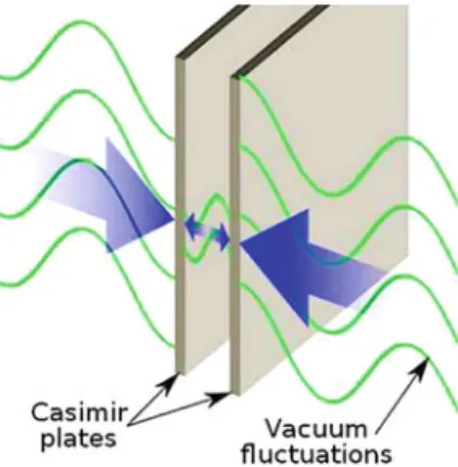
We discussed quantum tunnelling in Chapter 2, where we saw that wave- particle duality means that particles such as electrons can penetrate a potential barrier where this would

5 Variational Perturbation Theory 464 5.1 Variational Approach to Effective Classical Partition

Quantum physics or quantum mechanics * is the name given to the part of modern physics dealing with light and things that are very small—molecules, single atoms, subatomic

More generally, on the basis of this and other experiments, we must conclude that Maxwell’s equations are correct and that the speed of electromagnetic radiation is the same in

To summarize: In practice, by quantum field theory in curved space we will mean (1) propagating free quantum fields in a fixed background, or if we go one step further (2)

One can purely mathematical derive irreducible representations of a sym- metry group and label the energy levels with a quantum number this way.. This way one can also label

The topics covered include electrons, phonons, and their interactions, density functional theory, superconductivity, transport theory, mesoscopic physics, the Kondo effect and