Reconstruction of the 12‐lead ECG using a novel MR‐compatible ECG sensor network

HAL Id: hal-03211460

https://hal.univ-lorraine.fr/hal-03211460

Submitted on 29 Apr 2021

HAL is a multi-disciplinary open access

archive for the deposit and dissemination of

sci-entific research documents, whether they are

pub-lished or not. The documents may come from

teaching and research institutions in France or

abroad, or from public or private research centers.

L’archive ouverte pluridisciplinaire HAL, est

destinée au dépôt et à la diffusion de documents

scientifiques de niveau recherche, publiés ou non,

émanant des établissements d’enseignement et de

recherche français ou étrangers, des laboratoires

publics ou privés.

MR-compatible ECG sensor network

Jesús dos Reis, Paul Soullié, Julien Oster, Ernesto Palmero Soler, Gregory

Petitmangin, Jacques Felblinger, Freddy Odille

To cite this version:

Jesús dos Reis, Paul Soullié, Julien Oster, Ernesto Palmero Soler, Gregory Petitmangin, et al..

Recon-struction of the 12-lead ECG using a novel MR-compatible ECG sensor network. Magnetic Resonance

in Medicine, Wiley, 2019, 82 (5), pp.1929-1945. �10.1002/mrm.27854�. �hal-03211460�

Reconstruction of the 12-lead ECG using a novel

MR-compatible ECG sensor network

Jesús E. Dos Reis,

_{Paul Soullié,}

_{Julien Oster,}

_{Ernesto Palmero Soler,}

_Gregory

Petitmangin,

Jacques Felblinger,

and Freddy Odille

INTRODUCTION

Electrocardiography (ECG) devices in the MR scan room are required for monitoring specific patient populations (e.g. pediatric or unstable patients) and when the MR examination is performed under anesthesia (1). Furthermore it is the reference standard device for real-time synchronization of imaging sequences to the heart rate. Nevertheless ECG devices used in MRI differ from conventional ones used in general cardiology, such as diagnostic 12-lead ECG devices. This is due to the physical and technical constraints imposed by the MR electromagnetic fields. The use of radio-frequency (RF) fields implies potential hazards with long conducting cables (relative to the RF wavelength) placed close to the RF emission coil, as the local heating can result in patient burns (2). Most commercially available MR-compatible ECG systems use short cables from the electrodes to an ECG box, placed on the patient, where the signal is amplified, digitized and transferred safely, i.e. by optical or wireless transmission (1,3,4). Only a reduced number of electrodes is used (2 to 4), resulting in non-conventional leads. Furthermore, when the patient is placed inside the MR magnet, the ECG is distorted due to the magnetohydrodynamic (MHD) effect (5) (mainly during systolic ejection). Finally, when MR sequences are played, magnetic field gradient switching can cause artifacts on the ECG. To minimize the latter effect, the ECG is acquired with a narrow bandwidth (typically between 0.5Hz and 20-60 Hz). However this does not eliminate all gradient-induced artifacts which are in the range of 0 to 15 kHz. Real-time signal processing methods have been proposed to minimize both gradient-induced (6–13) and MHD-induced (11,14) artifacts. Radiofrequency shielding of the sensor box and low-pass filtering are also used to eliminate RF-induced ECG artifacts.

Conventional 12-lead ECG devices use a standardized electrode placement (10 electrodes). This standardized placement is especially useful for interpreting/localizing the origin of arrhythmias for diagnosis or treatment purpose, e.g. during catheter ablation procedures. When the acquisition bandwidth is 0.05 to 150 Hz, the ECG quality is of diagnostic quality. When it is lower, as in current MR-compatible devices (0.5 to 20-60 Hz), it is considered of monitoring quality. Monitoring quality allows heart rate analysis, but only diagnostic quality allows accurate measurement of certain features such as ST segment elevation during a stress test (15). Applying these definitions to MR-ECG is however not straightforward, as residual artifacts from gradient-induced and MHD-gradient-induced voltages often result in marked changes of the ECG morphology, even at the monitoring bandwidth. Therefore it may be more convenient to define ECG signal quality in MRI using objective similarity metrics (the correlation coefficient is used in this study) in comparison to a gold standard ECG acquired outside MRI (either at diagnostic or monitoring bandwidth).

Advanced cardiac MRI applications may benefit from a standard 12-lead ECG acquisition simultaneous to the imaging. Catheter interventions performed under MRI guidance have been shown feasible for arrhythmia ablation (16,17). Such procedures would definitely benefit from having a safe 12-lead ECG with diagnostic or near-diagnostic quality. An MR-conditional system has been proposed for use with 1.5 T interventional scanners (11). This ___________________________________________________

1_{IADI, INSERM and Université de Lorraine, Nancy, France;}

2_{Schiller Medical SAS, Wissembourg, France;}

3_{CIC-IT 1433, INSERM, Université de Lorraine and CHRU Nancy,}

Nancy, France;

This study was funded by the French "Investments for the Future" program under grant number ANR-15-RHU-0004, and by the European Commission through the Eurostars programme, grant number 9799 (ALVALE project: Anatomical Localization of the origin of Ventricular Arrhythmias from the 12-Lead ECG). The authors also thank INSERM, CPER 2007-2013, Région Lorraine and FEDER.

*Correspondence to: Freddy Odille, IADI, Inserm U947 CIC-IT 1433, Bâtiment Recherche, CHRU de Nancy Brabois, Rue du Morvan, 54511, Vandoeuvre-lès-Nancy, France. E-mail: freddy.odille@inserm.fr.

Purpose: Current electrocardiography (ECG) devices in MRI use non-conventional electrode placement, have a narrow bandwidth and suffer from signal distortions including magnetohydrodynamic (MHD) effects and gradient-induced artifacts. In this work a system is proposed to obtain a high quality 12-lead ECG.

Methods: A network of N electrically independent MR-compatible ECG sensors was developed (N=4 in this study). Each sensor uses a safe technology - short cables, pre-amplification/digitization close to the patient and optical transmission - and provides 3 bipolar voltage leads. A matrix combination is applied to reconstruct a 12-lead ECG from the raw network signals. A subject-specific calibration is performed to identify the matrix coefficients, maximizing the similarity with a true 12-lead ECG, acquired with a conventional 12-lead device outside the scan room. The sensor network was subjected to radiofrequency heating phantom tests at 3T. It was then tested in 4 subjects, both at 1.5T and 3T.

Results: Radiofrequency heating at 3T was within the MR-compatibility standards. The reconstructed 12-lead ECG showed minimal MHD artifacts and its morphology compared well with that of the true 12-lead ECG, as measured by correlation coefficients above 93% (respectively 84%) for the QRS complex shape during SSFP imaging at 1.5T (respectively 3T).

Conclusion: High quality 12-lead ECG can be reconstructed by the proposed sensor network at 1.5T and 3T with reduced MHD artifacts compared to previous systems. The system might help improve patient monitoring and triggering, and might also be of interest for interventional MRI and advanced cardiac MR applications.

Keywords: Electrocardiography (ECG), Electromagnetic Compatibility, Optical Sensor.

technology uses long coaxial cables (several meters) from the electrode clips to the exit of the scan room’s Faraday cage. In order to minimize induced RF in the cables, the coaxial cable shield was connected to DC-blocking capacitors and grounded to the scan room’s penetration panel, and ferrite chokes were mounted at specific points of the cables (beyond the 5-Gauss line). However this technology does not eliminate all risks of heating. Furthermore the long cable distance from the electrode to the amplification module results in a signal-to-noise ratio penalty and increased RF- and gradient-induced artifacts on the ECG signal, compared to conventional MR-compatible ECG devices. This system did include real-time signal processing methods for gradient artifact and MHD reduction, and was demonstrated to provide clinically useful signals for interventional MR applications. However the large distances between electrodes in a 12-lead setup result in high MHD voltages which cannot be completely suppressed, even with state-of-the-art modelling and signal processing (11,14).

In this work a network of ECG devices is proposed, comprised of several electrically independent sensors using a conventional MR-compatible technology (i.e. short cables, digitization close to the patient and optical transmission). The objective of the study is to show the feasibility of reconstructing a high-quality 12-lead ECG, using a linear combination of the sensor network’s raw signals. A calibration procedure is described to best fit the true 12-lead ECG, on a subject-specific basis, while minimize MHD artifacts. The proposed setup is shown to be particularly efficient in terms of MHD voltage reduction, due to the use of short distances between electrodes and due to a smart combination of the raw signals. The sensor network is tested in subjects in both 1.5T and 3T scanners. Validation is achieved by comparing the MRI 12-lead ECG to a conventional 12-12-lead ECG (acquired outside the scan room prior to MR scanning). The preservation of the morphology of the main ECG waves (P, Q, R, S, T) is analyzed.

METHODS

ECG Sensor Network

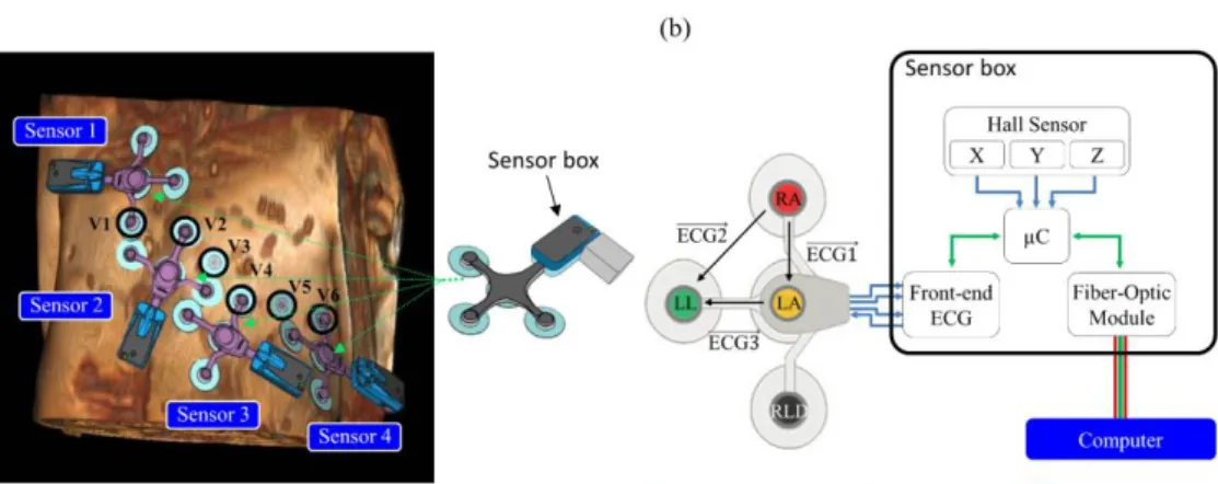
The ECG sensor network was comprised of N (N = 4 in this study) independent devices compatible with MRI (ECG sensor prototype based on the technology of the Maglife system, Schiller Medical, Wissembourg, France). The electronic design architecture of the device is shown in Fig. 1. Each device consisted of a flexible patch with three short branches protected against defibrillator shocks, allowing four electrode supports (one common lead reference electrode + three measurement electrodes) to be connected to the sensor box. The sensor provided three independent bipolar ECG leads with a bandwidth of 0.04 - 150 Hz and a raw resolution of 3.27 µV/LSB at 19 bits (the recalculated resolution is 1 µV/LSB at 16 bits, usable input dynamic ± 500 mV). The analog signals were first pre-amplified and digitized in an ECG front-end

module with 2 kHz sampling frequency, resampled at 1 KHz (ADAS1000BCPZ, Analog Devices Inc, Norwood, USA). Note the ECG front-end module used oversampling; details regarding the anti-aliasing filtering/undersampling stages are given in the Supporting Information document. The sensor box also integrated three Hall effect probes with a usable resolution of 659 uV/LSB at 12 bits, and a usable input dynamic of ± 1.35 V (CYSJ362A, ChenYang Technologies, Finsing, Germany) to measure the local magnetic field change in X, Y, Z (during switching of MR gradients) with a sampling frequency of 1 kHz and a microcontroller allowing real-time processing (gradient artifact denoising and QRS detection). Note that for this study, real-time gradient artifact denoising was disabled (offline correction was applied instead) in order to record the raw data and quantify ECG signal with/without artifact reduction. The signals were finally modulated and transferred by optical fiber from the sensor box to a computer (RS232 serial communication protocol from the microcontroller to the optical emission module at 460800 Baud).

RF Heating Experiments in Phantoms

The risk of overheating wires is a key topic in MR safety. The temperature increase in lead wires does not only depend on the type of material but also on the length and position within the RF emission coil, which can result in an antenna effect (23.4 cm at 1.5 T, i.e. for f = 64 MHz; 11.7 cm at 3 T, i.e. for f =128 MHz).

RF heating of the sensor network was investigated with an ASTM phantom following the CEI 60601-2-33 standard, on a Discovery MR750 3T scanner (General Electric, Milwaukee, USA). Temperatures were measured with ReFlex optical probes (Neoptix Inc, Quebec, Canada). This device has a precision of ± 0.8°C. To mimic the thermal and electrical properties of human skin, a semi-rigid conductive gel was made. The recipe for this gel was as described in ASTM F 2182A, i.e. 98.9% deionized water, 0.13% NaCl and 0.99% polyacrylic gel (commonly called PAA).

Two spatial configurations of the sensors were tested as shown in Supporting Information Figure S1a and Supporting Information Figure S1b. In order to maximize the antenna effect, electrodes were shared between the individual sensors (unlike in the subject experiments where each sensor was independent). The sensors were placed in a way to maximize the tangential electric field, based on simulated electric field maps, computed from a model of birdcage RF emission coil with an electromagnetic simulation software (CST, Darmstadt, Germany). The temperature probes were placed under the transparent conducting gel of the electrode (see Supporting Information Figure S2c). Temperatures were recorded for 3 min without any sequence in order to have a stable baseline, then for 15 min with an RF-intensive sequence (maximal transmit gain was set), and then again for 5 min without the sequence. Due to the limited number of temperature probes (N = 4), the measurement cycle 3min / 15min / 5min was applied 4 times for each configuration (see Fig. S2a and S2b).

Figure 1. (a) Positioning of the MR-compatible ECG sensor network on

the volunteer (the

conventional precordial

electrodes V1 to V6 are highlighted) and schema

of an ECG sensor

including the optical fiber transmission module (light gray). (b) Electronics design of the proposed ECG device and measured ECG leads.

Volunteer Experiments

ECG acquisitions were obtained on four healthy volunteers (3 males and 1 female, age range 29-56 years old, weight range 58-95 kg). Each subject underwent our experimental protocol on both a 1.5T AvantoFit scanner and a 3T Prisma scanner (Siemens, Erlangen, Germany). This study was approved by an ethics committee and all subjects gave informed written consent (ClinicalTrials.gov identifier: NCT02887053). A total of 22 MRI-compatible electrodes were placed on the subject (10 electrodes for calibration with the 12-lead standard ECG + 12 extra electrodes for the ECG sensor network).

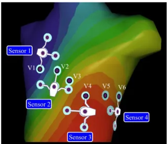
The experimental configuration was as follows. The subject first lay on the MR examination table, in the MRI preparation room (i.e. outside the scan room). Ten MR-compatible electrodes were placed on the chest and limbs of the subject (LA, RA, LL, RL, V1 to V6). A conventional 12-lead ECG device (Physiogard Touch 7, Schiller Medical, Wissembourg, France) was connected to these 10 electrodes and a reference 12-lead recording was acquired. Then the 12-lead device was disconnected and the N=4 MR-compatible ECG sensors were placed. Each sensor was placed in a way to reuse one of the precordial electrodes already in place (sensor 1: V1; sensor 2: V2; sensor 3: V4: sensor 4: V6), as shown in Fig. 1. Therefore 12 additional electrodes needed to be placed (3 extra electrodes per sensor). This setup has several advantages: it ensures multiple electrical projections are acquired, rotating around the heart; it makes use of the conventionally used electrode placement by reusing some of the precordial leads, while leaving some flexibility for the placement of other electrodes to adjust to the patient morphology; this setup is feasible with women, avoiding electrodes on the breasts (one of the volunteers was a female). Note that the setup does not have to be reproducible from one subject to another since a subject-specific calibration is performed hereafter. A recording was done with the sensor network in the preparation room. Then the examination table was entered into the scan room. Another recording was done with the sensor network, with the subject’s chest placed at the isocenter of the scanner, as for conventional cardiac examinations, before any sequence was played.

Additionally, in one of the subjects, a 12-lead ECG was acquired with the subject placed inside the MR scanner (both at 1.5 T and 3 T), using the conventional 12-lead device. The device monitor was kept outside of the 40 mT line (i.e. at the end of the examination table) to avoid attraction by the magnet and dysfunctioning, and no MR sequence was played in this setup for safety reason. This allowed a direct comparison of the MHD voltages with a conventional 12-lead system and with the proposed system.

The MRI acquisition protocol included sequences to test the robustness of the reconstructed 12-lead ECG during MRI scanning: first a typical sequence used in cardiac imaging, i.e. a cine balanced steady-state free precession (SSFP) sequence (TRUFI, acquisition matrix 224x208, slice thickness = 10 mm, flip angle = 40°, TE/TR=1.3/3.1 ms) and then a sequence providing worst-case gradient switching artifacts, i.e. a diffusion-weighted echo planar imaging sequence (DW-EPI, acquisition matrix 192x156, slice thickness = 5 mm, EPI echo train length = 59, 6 diffusion directions, B-value = 1000). These DW-EPI settings provided a combination of fast gradient switching (EPI train) and strong diffusion gradient pulses (approximately 20 ms plateaus) applied in all three spatial directions, including combinations of them (i.e. oblique gradient directions). Furthermore a T1 weighted sequence

(axial Dixon VIBE, FOV 410x410x350 mm3_{, 1.2x1.2x4 mm}3₎

covering the whole torso was included in order to have a geometrical model of the subject’s torso.

Raw ECG data from the 12-lead device were exported to a USB memory stick. Raw data from the sensor network, including ECG and Hall effect probes (X,Y,Z), were saved to hard disk on the acquisition computer. All signal processing tasks described hereafter, for 12-lead reconstruction, ECG denoising and

quantitative analysis, were performed offline using MATLAB (Mathworks, Natick, USA).

Twelve-lead ECG Reconstruction Minimizing MHD Effects

The 12-lead ECG reconstruction method used a method similar to that described in Refs. (18,19). It is based on the assumption that the conventional 12-lead ECG 𝑉12𝐿𝑒𝑎𝑑(𝑡) can be estimated by a

linear transformation of the signals from the sensor network 𝑉𝑁𝑒𝑡𝑤𝑜𝑟𝑘(𝑡), as described by a matrix M in the equation below :

𝑉12𝐿𝑒𝑎𝑑(𝑡) = 𝑀 × 𝑉𝑁𝑒𝑡𝑤𝑜𝑟𝑘(𝑡) (1)

Here 𝑉12𝐿𝑒𝑎𝑑(𝑡) is a vector of 12 elements representing one time

sample. 𝑉𝑁𝑒𝑡𝑤𝑜𝑟𝑘(𝑡) is a vector of 3N elements (N sensors, each

providing 3 bipolar leads, 3N=12 in this study). The M matrix is therefore of size 12x12 and is determined on a subject-specific basis, in a calibration step described hereafter.

The calibration step used one 12-lead recording and one sensor network recording, which did not need to be acquired simultaneously. The processing consisted of the following steps: (i) QRS peak detection on 𝑉12𝐿𝑒𝑎𝑑 and on 𝑉𝑁𝑒𝑡𝑤𝑜𝑟𝑘 (QRS detection

library of the PB1000 ECG device, Schiller Medical, Wissembourg, France) ; (ii) slicing of 𝑉12𝐿𝑒𝑎𝑑 and 𝑉𝑁𝑒𝑡𝑤𝑜𝑟𝑘 signals

into a number N1 and N2 of cardiac cycles respectively ; (iii) robust

averaging of all cardiac cycles, using the median over the N1

(respectively N2) cardiac cycles, providing < 𝑉12𝐿𝑒𝑎𝑑> and <

𝑉𝑁𝑒𝑡𝑤𝑜𝑟𝑘> templates ; (iv) regularized inversion of system (1),

rewritten in the form 𝐴𝑀 = 𝑏 (with A and b constructed from the template signals, see detailed description in Appendix A), i.e. 𝑀 = (𝐴𝑇_{𝐴 + 𝜆𝐼)}−1_𝐴𝑇_{𝑏 (Tikhonov regularization, with 𝐼 the identity}

matrix). The regularization parameter 𝜆 was set to 10−2 for the whole study. This was to prevent overly noisy leads in 𝑉𝑁𝑒𝑡𝑤𝑜𝑟𝑘 to be given a large weight in the reconstruction. Since the QRS peak detection was performed on different lead systems, the < 𝑉12𝐿𝑒𝑎𝑑> and < 𝑉𝑁𝑒𝑡𝑤𝑜𝑟𝑘> templates may be slightly

misaligned. Therefore the reconstruction was performed after a variable time shift (from -40 ms to + 40 ms with steps of 1 ms). The time shift providing the most accurate reconstruction was kept, defined as the one providing the best correlation coefficient on the QRS complex (i.e. a 120 ms window centered at the QRS peak).

Two calibration strategies were tested: (Cout) calibration using

the 𝑉𝑁𝑒𝑡𝑤𝑜𝑟𝑘 signals recorded outside the scan room (in the

preparation room) and (Cin) calibration using the 𝑉𝑁𝑒𝑡𝑤𝑜𝑟𝑘 signals recorded inside the scanner, i.e. when the subject was placed at the isocenter of the magnet (with no sequence played). The difference between the two strategies is that in Cin, the 𝑉𝑁𝑒𝑡𝑤𝑜𝑟𝑘 signals are corrupted by MHD artifacts. As a consequence, the M matrix provides a linear combination of 𝑉𝑁𝑒𝑡𝑤𝑜𝑟𝑘 signals that intrinsically

minimizes MHD artifacts, to best fit < 𝑉12𝐿𝑒𝑎𝑑>. By contrast,

calibration Cout provides an M matrix that is blind to the

propagation of MHD artifacts, therefore the reconstruction is likely to amplify MHD effects when the subject is subsequently placed in the MRI bore.

Gradient-induced Artifact Reduction

We aimed to check that the proposed 12-lead reconstruction method can be combined with existing methods for gradient artifact reduction. To this end a previously published correction method was applied to the raw signals (before combination into the 12-lead reconstruction). In particular we meant to check how the residual artifacts propagated into the reconstruction. Gradient-induced artifacts on the ECG during the SSFP sequences were reduced by simple band-pass filtering with cut-off frequencies of 0.5-30 Hz (zero-phase digital butterworth 4th _{order filter, i.e.}

forward-backward filtering). For the DW-EPI sequences, the band-pass filtering was not sufficient. Therefore gradient-induced artifacts were reduced using a previously described adaptive filtering technique (7,13). Details of the method are given in the Supporting Information document.

Quantitative ECG Morphology Analysis

The fidelity of the reconstructed ECG morphology was quantified using correlation coefficient metrics. ECG waves were assumed to be highly reproducible over the duration of the exam in our healthy subject population. The template 12-lead ECG < 𝑉12𝐿𝑒𝑎𝑑>, constructed during the calibration procedure, was used

as a reference for comparison. Each heart beat of the reconstructed 12-lead ECG was then compared to the reference with Pearson’s correlation coefficient, calculated for each of the 12 leads. Statistics of these correlation coefficients were computed over the duration of the following recordings: (i) in the preparation room; (ii) inside the MR bore; (iii) during the cine SSFP sequence; (iv) during the DW-EPI sequence. Correlation coefficients were computed on the whole PQRST wave (window duration set to 80% of the median cardiac cycle, starting 200 ms before the detected QRS peaks) and on the QRS complex (window duration set to 120 ms, centered at the QRS peaks). A manual correction of the QRS peak detection was done when necessary before computing all the statistics. For SSFP and DW-EPI recordings, only heart beats during actual gradient pulsing were analyzed.

Monte-Carlo Simulation of Pathological ECG Changes and MHD changes

The experiments in healthy volunteers did not include significant changes in the ECG morphology during the course of the acquisition. They also did not include significant changes in the MHD morphology, which can happen if the cardiac output flow pattern changes, as in the case of a stress test. Furthermore the robustness to electrode placement was not investigated thoroughly in the subjects. Indeed with the proposed placement there are a number of degrees of freedom for connecting each sensor to the four chosen precordial electrodes (V1, V2, V4, V6). Therefore changes in both ECG morphology and MHD morphology were assessed by a Monte-Carlo simulation, designed to test random variations of electrode placement.

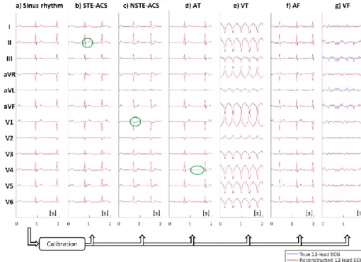
In order to test the robustness of the 12-lead reconstruction method to sudden changes in ECG morphology, a numerical simulation was performed. The simulation consisted of a 3D torso model providing body surface potential maps (BSPM) of different ECG morphologies (see Fig. 2). The BSPM were generated by spline interpolation of the unipolar voltages from synthetic 12-lead ECG signals, which were generated by an ECG simulator device (MS 410, MedTec & Science GmbH, Ottobrunn, Germany). In this 3D numerical model, electrodes from the 12-lead ECG and from the proposed sensor network (N=4 sensors) were placed in a way to mimic the configuration used in the volunteer experiments. The Monte-Carlo scheme consisted of repeating the experiments with random variations of the electrode placements, under the constraint that one measurement electrode of each sensor was placed on V1, V2, V4 and V6 (for sensor 1, 2, 3, 4 respectively). This means that, for each sensor (3 measurement electrodes): the electrode connected to the precordial lead was randomly drawn; a rotation by a random angle about the torso surface normal vector was applied. Bipolar voltages from the proposed sensors were then synthetized by difference of the BSPM values at the corresponding electrode positions. The following ECG morphologies were synthetized: normal sinus rhythm (SR), ST-elevated acute coronary syndrome (STE-ACS), non-ST-elevated acute coronary syndrome (NSTE-ACS), atrial tachycardia (AT), ventricular tachycardia (VT), atrial fibrillation (AF) and ventricular fibrillation (VF). SR signals were used for calibration, and the resulting 𝑀 matrix was subsequently applied to reconstruct 12-lead signals during STE-ACS, NSTE-ACS, AT, VT, AF and VF, thus simulating a wide range of morphological changes occurring after the calibration step. The quality of the reconstruction was assessed by computing correlation coefficients between the true and reconstructed 12-lead ECG signals for each morphology. The number of Monte-Carlo

experiments was set to 𝑁𝑒𝑥𝑝= 50 in order to have a wide range of

electrode placement variations.

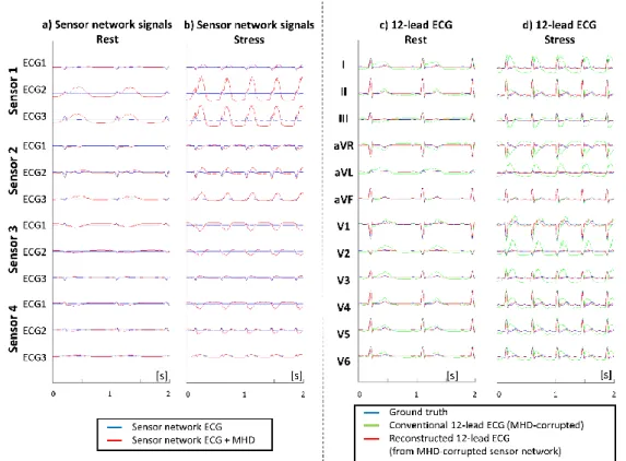
In order to test robustness to sudden changes in MHD morphology, we performed additional simulations incorporating an MHD signal model. The MHD signal was generated using a previously published model (14), based on a geometrical model of the aortic arch and aortic flow curves, as measured by phase-contrast MRI across the aortic arch. Two MHD models were generated: a model at rest which was added to an SR ECG at 60 bpm, and a model at stress, which was added to an SR ECG at 120 bpm (using a cardiac output factor of 1.9 compared to rest). In order to simulate a worst-case scenario, the amplitude of the MHD signals resulting from the aortic arch model were scaled by a factor of 5, which visually seemed to correspond to worst case recordings at 3T. Both the shape and amplitude of the MHD signal were markedly changed between rest and stress. Signals obtained in SR at 60 bpm (with added MHD model at rest), were used for calibration, and the resulting 𝑀 matrix was subsequently applied to reconstruct 12-lead signals during stress (SR signal at 120 bpm with added MHD model at stress). The quality of the reconstruction was assessed by computing correlation coefficients between the ground truth 12-lead ECG, the MHD-corrupted 12-lead ECG and reconstructed 12-lead ECG signals. Here again the Monte-Carlo scheme was used to vary electrode placement (𝑁𝑒𝑥𝑝= 50).

RESULTS

RF Heating Results

The ASTM phantom experiments at 3T showed a temperature increase between 1.2 °C and 4.6 °C (± 0, 8 °C) for the first spatial configuration (Fig. S2a) and between 2.4 °C and 4.7 °C (± 0.8 °C) for the second configuration (Fig. S2b). In both configurations, the largest temperature increase was recorded at the common lead electrode that was located farthest from the center, i.e. closest to the RF emission coil.

Volunteer Experiment Results

The experimental protocol was successfully applied to all 4 subjects at both 1.5 T and 3 T. Complete datasets were obtained in all cases, including 12-lead reference and network signals outside/inside the scanner and during MR scanning.

Figure 2. The 3D model used for numerical simulation of different ECG morphologies. The body surface potential map (BSPM) is synthetized by interpolation of the unipolar voltages from the 12-lead ECG. Sensor network signals are synthetized by local bipolar voltage measurements from the BSPM, using virtual electrodes located as in the volunteer experiments.

The calibration procedure to calculate the 𝑀 matrix for a given subject and scanner took approximately 1 s with MATLAB code.

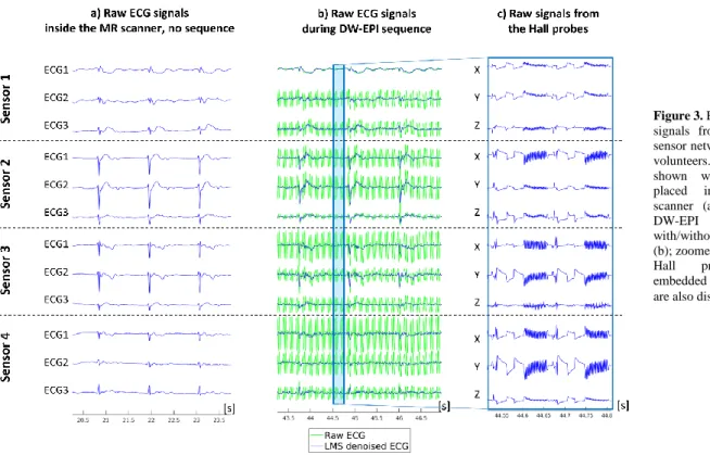
Exemplary raw signals from the sensor network are displayed in Fig. 3, i.e. before 12-lead reconstruction. Fig. 3 shows signals acquired with the subject placed inside the MR scanner (no sequence played), and during a DW-EPI sequence (with and without LMS denoising). Zoomed signals from the Hall probes (X,Y,Z probes from each sensor box) are also displayed and show characteristic magnetic field changes occurring during this sequence, including a wide bipolar diffusion encoding gradient set followed by a fast switching EPI gradient pattern (two repetition times shown in Fig 3c).

Exemplary 12-lead ECG reconstructions of one subject are given in Fig. 4 (1.5 T) and Fig. 5 (3 T). Detailed versions of these two figures (with all 12 leads) are shown as Supporting Information Figures S3 and S4. The two calibration strategies Cout and Cin are

shown. It can be seen that, when the calibration matrix 𝑀 was calculated using Cout calibration (i.e. from the network recording

outside the scanner) the most accurate reconstruction was achieved in the preparation room and provided an excellent match; however when the patient was placed in the scanner, the best reconstruction was found with Cin (i.e. from the recording with the subject at the

magnet isocenter). When using Cin calibration, the residual MHD

artifact was of small amplitude in all 12 reconstructed leads at 1.5 T and resulted in a more conventional T-wave morphology. At 3 T, the T-wave remained distorted compared to the conventional 12-lead reference, but the MHD artifact was markedly reduced compared to using Cout calibration. The corresponding calibration

matrices show which signals from the sensor network did contribute to each of the reconstructed 12 leads. All signals from the network were used in these two examples. The difference in 𝑀 coefficients between Fig. 4a and Fig. 5a, when using Cout

calibration, is indicative of the variability of the calibration procedure due to the variability of electrode positioning in two different sessions. The contribution from each lead of the sensor network, in terms of energy ratio (i.e. energy of the contribution of a particular leadto the 12-lead reconstruction, normalized by the energy of the 12-lead ECG: ‖𝑉_{𝑁𝑒𝑡𝑤𝑜𝑟𝑘}(𝑙𝑒𝑎𝑑) × 𝑋(𝑙𝑒𝑎𝑑)‖ ‖𝑉⁄ 12𝐿𝑒𝑎𝑑‖), is

given in the Supporting Information Table S2. Only in one subject

at 3T, one sensor did not contribute to the reconstructed 12-lead ECG, but in general, all raw leads had a significant contribution. Note that the sum of energy contributions of all leads for one subject is not equal to 100% since the contributions from all leads can add up constructively of destructively according to the sign of the matrix coefficient.

Differences in MHD voltage amplitudes are shown in the Supporting Information Figure S5. The figure shows both the raw and reconstructed signals from the sensor network, which are to be compared to the ECG obtained with a conventional 12-lead device, both at 1.5 T and 3 T. The conventional device showed the largest MHD voltages. The raw network signals also showed MHD voltages of reduced amplitude, as expected from the shorter distances between electrodes. The reconstructed 12-lead signals showed a further reduction of MHD voltages. These observations were quantified in the Supporting Information Table S1, which show a gradual improvement in correlation coefficients from the conventional 12-lead device (59.1% / 32.3% at 1.5 T / 3 T respectively) to the reconstructed 12-lead ECG (92.4 % / 77.9 % respectively).

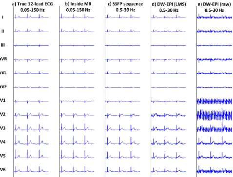
Example reconstructed signals during MRI sequences are shown in Fig. 6 in one subject at 1.5 T. Despite the residual MHD effect, the overall shape of the signals seemed well preserved in the reconstructed ECG, as well as the relative changes between leads, especially from V1 to V6. When sequences were played, the morphology was further affected by gradient-induced artifacts, but these were minimized by the filtering to the monitoring bandwidth of 0.5-30 Hz (which was sufficient in SSFP sequences) and by the LMS adaptive denoising in worst-case sequences (DW-EPI). As a result of the bandwidth narrowing, the amplitude and sharpness of the QRS complexes were slightly decreased compared to the true 12-lead ECG.

Figure 3. Example raw ECG signals from the proposed sensor network in one of the

volunteers. Signals are

shown with the subject

placed inside the MR

scanner (a) and during a

DW-EPI sequence

with/without LMS denoising (b); zoomed signals from the

Hall probes (X,Y,Z)

embedded in each sensor box are also displayed (c).

Figure 4. Example reconstructed 12-lead ECG of a subject at 1.5 T inside the MR scanner (template ECG cycle, precordial leads shown). The superimposed true (blue) and reconstructed (red) 12-lead ECG signals are shown: (a) after

calibration Cout (i.e. matrix computed from the sensor network signals recorded

outside the scanner); (b) after calibration Cin (i.e. from the sensor network

signals recorded inside the scanner). The corresponding calibration matrices are shown for Cout (c) and Cin (d) calibration. The full ECG datasets are shown in

Supporting Information Figure S3.

Figure 5. Example reconstructed 12-lead ECG of a subject at 3 T inside the MR scanner (same subject as in Fig. 5, precordial leads shown). The superimposed true (blue) and reconstructed (red) 12-lead ECG signals are shown: (a) after calibration Cout (i.e. matrix computed from the sensor network

signals recorded outside the scanner); (b) after calibration Cin (i.e. from the

sensor network signals recorded inside the scanner). The corresponding calibration matrices are shown for Cout (c) and Cin (d) calibration. The full

ECG datasets are shown in Supporting Information Figure S4.

Figure 6. Example 12-lead ECG of a subject: true 12-lead ECG acquired

outside the scanner (a);

reconstructed 12-lead ECG from the sensor network at 1.5 T, inside the scanner (b), during an SSFP cine sequence (c), during a DW-EPI

sequence with LMS adaptive

filtering (d) and without LMS filtering (e). Note the bandwith was 0.05-150 Hz when no sequence was played, and 0.5-30 Hz during MR sequences.

Quantitative ECG Morphology Results

Quantitative analysis of the reconstructed ECG morphology is summarized in Table 1. The correlation coefficient with the true 12-lead ECG template is indicated for the different experimental setups (outside/inside MR and during sequences) and calibration modes. Note that the bandwidth of the reconstructed ECG was 0.05-150 Hz (diagnostic quality) when no sequence was played and was 0.5-30 Hz when sequences were played (monitoring quality). Reconstruction outside the scanner, using Cout calibration,

showed excellent correlation scores (above 96%). This supports the initial assumption that the conventional 12-lead ECG can be reconstructed accurately by linear combinations of multiple bipolar voltage measurements.

Reconstructions inside the scanner allowed MHD artifacts to be quantified through the decrease of correlation coefficients on the PQRST wave, compared to the first row of the table. It can be seen that Cin calibration indeed minimized MHD artifact propagation in

the reconstruction compared to Cout (88.7% instead of 80.1% at 1.5

T, 75.9% instead of 64.6% at 3 T). While residual MHD effect prevented perfect 12-lead ECG reconstruction, a relatively good preservation of the QRS complex morphology was able to be

achieved, with correlation scores of 95.6% at 1.5 T and 90.5% at 3 T. When SSFP sequences were played, there was a larger decrease of correlation scores, which was expected due to the bandwidth restriction (0.5-30 Hz), applied to minimize gradient-induced artifacts. Finally, when worst-case sequences were played (DW-EPI), correlation scores were reduced further, especially when no LMS correction was used. Correlation scores after LMS were still below those measured in SSFP sequences, which was expected as the LMS filter generally needs a few cardiac cycles to adapt its coefficients. The statistics presented in Table 1 did take into account all heart beats acquired during the DW-EPI sequence, including the early ones were the LMS filter had not converged to its optimal.

Monte-Carlo Simulation Results

Results from the simulation with different ECG morphologies are shown in Fig. 7 for an electrode placement close to that used in the subject experiments. It can be seen that the 12-lead reconstruction was robust to morphologic changes when the

Figure 7. Results of the numerical simulation, showing the robustness of the 12-lead reconstruction to changes in ECG morphology. The true (blue) and reconstructed (red) 12-lead ECG signals are shown during sinus rhythm, which is used for calibration of the M matrix (a). The same M matrix is subsequently used to reconstruct the following pathological ECG signals: ST-elevated acute coronary syndrome (b), non-ST-elevated acute coronary syndrome (c), atrial tachycardia (d), ventricular tachycardia (e), atrial fibrillation (f) and ventricular fibrillation (g).

Table 1. Correlation coefficient between the true and reconstructed 12-lead ECG in the healthy subjects, expressed as mean ± standard deviation over the

12 leads (averaged on N=4 subjects)

Calibration mode Experimental setup 1.5T 3T

PQRST QRS PQRST QRS Cout Outside MR (0.05-150 Hz) 97.0% (± 1.1%) 97.3% (± 1.4%) 96.7% (± 1.8%) 97.4% (± 1.7%) Inside MR (0.05-150 Hz) 80.1% (± 7.0%) 93.7% (± 4.0%) 64.6% (± 11.4%) 91.1% (± 3.7%) Cin Outside MR (0.05-150 Hz) 92.3% (± 3.5%) 95.6% (± 2.2%) 88.6% (± 5.2%) 92.2% (± 4.7%) Inside MR (0.05-150 Hz) 88.7% (± 2.5%) 95.6% (± 2.1%) 75.9% (± 6.4%) 90.5% (± 4.7%) SSFP sequence (0.5-30 Hz) 83.5% (± 4.5%) 93.2% (± 3.9%) 62.6% (± 5.4%) 84.9% (± 5.0%)

DW-EPI sequence, LMS corrected

(0.5-30 Hz) 71.6% (± 4.8%) 80.7% (± 4.8%) 34.9% (± 3.8%) 49.0% (± 4.9%)

DW-EPI sequence, uncorrected

calibration was performed during normal sinus rhythm. The reconstruction was nearly perfect in case of deflection of the ST segment (ST elevation or ST depression), as seen in STE-ACS and NSTE-ACS signals. The characteristic patterns of AT and VT were also well reconstructed in most leads. Except for leads III and aVL in the VT signals, the reconstructionwas nearly perfect and showed excellent preservation of the morphology, especially in precordial leads (V1 to V6). Typical patterns of AF and VF were

also well reconstructed and well recognized. Not surprisingly, the largest error was made for VF (which is the most incoherent activation pattern), but again, the error in precordial leads remained very small. Those qualitative results were confirmed by the correlation metrics which are summarized in Table 2. The means and standard deviations indicate statistics obtained for the 𝑁𝑒𝑥𝑝=

50 Monte-Carlo experiments, with varied electrode positions. The

Table 2. Correlation coefficient between the true and reconstructed 12-lead ECG, expressed as mean ± standard deviation over the Monte-Carlo simulations with

randomized electrode positions (𝑁𝑒𝑥𝑝= 50 experiments).

Lead SR _ACS STE- _ACS NSTE- AT VT AF VF

SR + MHD, rest SR + MHD, stress Recon. 12-lead(1) Conv. 12-lead(2) Recon. 12-lead(1) Conv. 12-lead(2) I 98.2% ±0.4% 97.9% ±0.5% 98.3% ±0.5% 98.0% ±0.5% 99.8% ±0.1% 96.8% ±1.8% 76.0% ±19.8% 97.6% ±1.6% 59.8% 92.5% ±4.9% 32.4% II 99.2% ±0.7% 99.1% ±0.7% 98.8% ±0.8% 99.2% ±0.8% 99.9% ±0.2% 98.5% ±2.4% 87.0% ±18.9% 99.0% ±1.5% 91.9% 96.6% ±4.6% 78.0% III 97.8% ±1.4% 97.7% ±1.5% 97.2% ±1.3% 97.7% ±1.6% 91.1% ±1.6% 94.7% ±3.1% 81.0% ±18.5% 97.5% ±1.4% 63.0% 95.8% ±3.7% 44.7% aVR 99.1% ±0.5% 98.9% ±0.6% 98.8% ±0.7% 99.0% ±0.6% 100.0% ±0.1% 98.4% ±2.2% 94.6% ±11.1% 98.8% ±1.5% 77.5% 95.7% ±4.7% 52.8% aVL 80.4% _±5.9% 80.4% _±5.8% 82.0% _±5.8% 78.7% _{±6.4% ±0.5%} 99.0% 74.7% _±6.8% 94.8% _±4.8% 73.3% _±4.7% 41.0% 46.7% _±6.8% 14.4% aVF 99.1% ±0.9% 99.0% ±1.0% 98.6% ±0.9% 99.1% ±1.0% 99.3% ±0.4% 98.0% ±2.6% 80.1% ±21.5% 98.9% ±1.4% 99.7% 97.1% ±4.3% 99.2% V1 89.2% ±4.8% 88.0% ±5.3% 83.4% ±4.9% 89.2% ±5.1% 99.9% ±0.1% 89.4% ±5.4% 89.6% ±11.0% 92.6% ±1.1% 93.0% 83.4% ±2.2% 88.1% V2 90.8% ±4.5% 89.2% ±5.0% 81.1% ±5.0% 90.8% ±4.7% 99.9% ±0.2% 90.1% ±5.3% 89.2% ±21.1% 93.6% ±1.0% 48.5% 85.8% ±1.9% 27.6% V3 98.4% ±0.4% 98.2% ±0.4% 97.4% ±0.5% 98.3% ±0.5% 99.9% ±0.1% 97.7% ±1.5% 80.9% ±17.2% 97.8% ±1.5% 62.1% 93.1% ±4.9% 34.5% V4 99.0% _±0.5% 98.9% _±0.5% 98.7% _±0.5% 98.9% _±0.6% 100.0% _±0.1% 98.6% _±1.9% 94.6% _±9.9% 98.7% _±1.5% 86.4% 95.4% _±4.7% 66.8% V5 98.9% ±0.5% 98.8% ±0.5% 98.6% ±0.4% 98.8% ±0.5% 100.0% ±0.1% 98.6% ±1.8% 93.5% ±9.5% 98.5% ±1.5% 81.7% 95.1% ±4.8% 59.2% V6 98.8% ±0.5% 98.6% ±0.5% 98.5% ±0.4% 98.7% ±0.5% 99.9% ±0.1% 97.8% ±2.3% 89.4% ±11.7% 98.4% ±1.5% 78.7% 94.4% ±4.8% 54.6% 12-lead average 95.8% ±1.2% 95.4% ±1.2% 94.3% ±1.2% 95.5% ±1.2% 99.0% ±0.2% 94.4% ±2.5% 87.6% ±9.5% 95.4% ±1.4% 73.6% 89.3% ±3.6% 54.4%

(1) _{Correlation coefficientbetween the reconstructed 12-lead ECG and the true 12-lead ECG}

(2) _{Correlation coefficientbetween the reconstructed MHD-corrupted 12-lead ECG and the true 12-lead ECG}

Figure 8. Results of the numerical simulation, showing the robustness of the 12-lead reconstruction to changes in MHD morphology. The true

(blue) and MHD-corrupted

(red) raw sensor network

signals are shown at rest (a) and during stress (b). The 12-lead ECG signals are shown at rest (c) and during stress (d), including the ground truth

(blue), the MHD-corrupted

ECG using conventional

electrode placement (green) and the proposed reconstruction (red). Here the M matrix was calibrated using the MHD-corrupted network signals at rest and the ground truth 12-lead ECG at rest; the same matrix M was then applied to the stress data for reconstruction.

largest error in the calibration was made for the estimation of lead aVL, which was also the lead with the lowest amplitude. These errors seemed to propagate in the reconstruction of other ECG morphologies, in particular of VF. For the particular electrode setup shown in Fig. 2, except for leads III and aVF, correlation coefficients were above 98% for the reconstruction of STE-ACS, NSTE-ACS, AT, VT and AF. For randomized electrode placements, the 12-lead average correlation was above 95% for all tested ECG morphologies (except for VF).

Results from the simulation with different MHD morphologies are shown in Fig. 8 for an electrode placement close to that used in the subject experiments. The MHD-corrupted signal showed that the simulation model was able to reproduce large amplitude MHD voltages resembling worst-case scenarios at 3T. These MHD signal were also very large in the raw network signals, although the distance between electrodes was short. The MHD artifact was markedly different in shape and amplitude between the rest and stress models. The 12-lead reconstruction showed a good minimization of the MHD effect compared to the conventional 12-lead ECG, though a residual mismatch of the T-wave could be seen. Quantitative measures are indicated in Table 2 (last four columns). Correlation scores for the calibration using the MHD-corrupted signals at rest were in line with the subject experiments, with a 12-lead average correlation of 95.4% (against 73.6% for a conventional 12-lead placement). During stress, the MHD-minimizing properties was still efficient, providing 89.3% correlation (against 54.5% for a conventional 12-lead placement).

DISCUSSION

This study shows the feasibility of obtaining a high quality 12-lead ECG from a network of MR-compatible ECG sensors utilizing short cables and pre-amplification/digitization close to the patient. The proposed method presently requires an extra acquisition step outside the scanner, with a conventional 12-lead ECG device, in order to identify a subject-specific calibration matrix. The results suggest identifying the calibration matrix from a network recording with the subject placed inside the MR bore, so that the calibration matrix can minimize MHD artifact propagation. The processing time for this calibration is short (approximately 1s) and the subsequent 12-lead ECG reconstruction is obtained by a simple linear combination of the raw network signals, which makes the method easily applicable in real-time. During worst-case sequences, gradient switching artifacts are still an issue, but such artifacts were able to be minimized through filtering and previously described adaptive denoising. The morphology preservation was quantified in terms of correlation coefficients of the QRS and PQRST waves, and showed good to excellent results for the QRS complex, even during scanning with conventional SSFP sequences ( > 93 % at 1.5 T, > 84% at 3 T). The robustness to sudden changes in the ECG morphology was shown in simulations, with only minor errors in specific leads for the most complex morphologies (VT, VF) which did not seem to affect the diagnostic value of the reconstructed signal. In particular, the baseline differences observed during ST elevation or ST depression were well reconstructed (in the absence of MHD artifact) and most of the morphologic changes in atrial and ventricular activation disorders were also well preserved. The robustness to sudden changes of the cardiac output flow pattern was also tested in a rest/stress simulation, as they result in changes in shape and amplitude of the MHD pattern. Though residual MHD artifacts were noticeable, they remained significantly reduced compared to the conventional 12-lead electrode placement setup, and 12-lead ECG signals were reconstructed with an accuracy of 89% on average during stress.

The sensor network was found to be safe at 3 T. Measured temperature elevations in the ASTM phantom experiments were below 5°C on average, which was below the thresholds defined by the CEI 60601-2-33 standard (43°C for devices in contact with

skin, skin temperature being in the range 33-37°C). The experiments were designed to obtain worst-case results. In the phantom experiments (unlike in the subjects), electrodes were shared between the different sensors, thus maximizing the effective length of the conducting wires, and thereby the RF antenna effect. To our knowledge, only an MR-conditional 12-lead ECG device was previously reported at 1.5 T (11), so the present work is the first report of a safe 12-lead ECG system operating at both 1.5 and 3 T.

A high-quality 12-lead ECG device in MRI may be beneficial in several applications. It might help improve patient monitoring, as the ECG signals can be displayed in a conventional lead system which is easier to interpret than non-standard leads. The main information that is required for ECG patient monitoring is the instantaneous heart rate. This relies on robust detection of the QRS peaks (20). Efficient synchronization of MR sequences also does. With all 12 leads being available, more robust QRS detection algorithms may be implemented, e.g. based on deep learning, or one could select one or several leads, e.g. with highest QRS amplitude or lowest amplitude of the MHD artifact, to be used as inputs of the QRS detector. The MHD artifact minimization, resulting from the proposed calibration strategy, may also improve the robustness of QRS detection. In this study 4 sensors were used, however a 12-lead ECG estimate could also be obtained from fewer sensors (even from only one sensor). Of course, with fewer sensors, a lower correlation with the true 12-lead ECG would be expected. The optimal placement of the sensors might be investigated based on the same methodology as described here. This would allow keeping the benefit of interpreting standardized leads with minimized MHD, with little or no extra hardware. In the case of only one sensor being used, more advanced reconstruction methods could be implemented such as artificial neural networks (21). To avoid excessive patient preparation time, a generic calibration strategy would be useful rather than the subject-specific calibration used here, which requires an additional recording in the preparation room with a 12-lead device.

Advanced applications in cardiac MRI may also benefit from the proposed system. Interventional MRI requires a clean ECG during imaging sequences. Rapid gradient echo sequences, such as the SSFP sequences tested here, are commonly used to track objects during the intervention (i.e. catheter, biopsy needle etc…). The device might also be of interest for cardiac stress testing MRI, as quantitative imaging parameters could be measured simultaneously or near-simultaneously with quantitative ECG metrics, such as ST elevation. However diagnostic quality ECG (0.05-150 Hz) would definitely be required, especially because restrictive high-pass filters do prevent the accurate measurement of subtle baseline differences. Specific applications such as arrhythmia ablation, performed under MRI guidance, also need a high quality ECG. Some of these catheter ablation techniques require a quantitative analysis of ECG morphology in order to locate the ablation target, such as the pace-mapping technique used for ventricular tachycardia ablation (22,23). Therefore a good preservation of the QRS morphology is essential. The main challenge to obtain a high-quality ECG for such applications may be the variability in the cardiac output flow pattern (between rest and stress, or during arrhythmic events), which leads to changes in MHD morphology. In our worst-case stress test simulation, the residual MHD artifacts remained of small amplitude, suggesting that the identified lead combination is relatively robust to changes in MHD morphology. However the method should be tested in actual patients in order to determine the true diagnostic value of the reconstructed signals.

Electrocardiographic imaging (ECGI), also called inverse cardiac activation mapping, is an emerging field in cardiology and is another potential application (24,25). ECGI consists of reconstructing a cardiac activation map from body surface potential measurements and from a torso model of the patient (including geometry, conductive properties, and location of electrodes), which can be obtained by imaging. Electrode vests have been developed

in the past years providing more than 200 electrodes (24). Such systems are not MR-compatible, so they have been used in combination with CT imaging. Meanwhile advanced optimization techniques have shown the feasibility of accurate activation mapping in PVC (premature ventricular contractions) from the standard 12-lead ECG (26). The proposed system might be a valuable tool in that field as it might improve the consistency between the ECG measurements and the imaging data, MRI being the reference standard imaging modality for cardiac tissue characterization.

CONCLUSION

Reconstruction of the 12-lead ECG has been shown feasible at 1.5 T and 3 T from a network of MR-compatible sensors. The system allows high quality 12-lead ECG to be obtained with minimal MHD artifacts, with a bandwidth of 0.05-150 Hz (when no sequence is played) or 0.5-30 Hz (during sequences). The system might be used to improve patient monitoring and sequence triggering in conventional MR examinations. It could be of interest for interventional MRI or for advanced cardiac MRI applications.

APPENDIX

A detailed description of the linear system 𝐴𝑀 = 𝑏 solved during the calibration process is given below. 𝐴 is a block diagonal matrix, composed of a block 𝐴̃ that is repeated along the diagonal:

𝐴 = [𝐴̃ ⋯ 0⋮ ⋱ ⋮ 0 ⋯ 𝐴̃ ] , 𝐴̃ = [𝑉12 (1)_(𝑡 1) ⋯ 𝑉12(12)(𝑡1) ⋮ ⋱ ⋮ 𝑉₁₂(1)(𝑡𝐾) ⋯ 𝑉12(12)(𝑡𝐾) ]. (A1)

Coefficients 𝑉₁₂(𝑙)(𝑡𝑘) represent the signal from the 12-lead ECG

measured by lead 𝑙 (𝑙 = 1 … 12) and time 𝑡𝑘 (𝑘 = 1 … 𝐾, where 𝐾

is the number of samples in the template ECG cycle).

The 𝑏 vector is a concatenation of the sensor network signals:

𝑏 = [ [𝑉𝑁𝑒𝑡𝑤𝑜𝑟𝑘 (1) _(𝑡 1) ⋮ 𝑉_{𝑁𝑒𝑡𝑤𝑜𝑟𝑘}(1) (𝑡𝐾) ] ⋮ [𝑉𝑁𝑒𝑡𝑤𝑜𝑟𝑘 (12) _(𝑡 1) ⋮ 𝑉_{𝑁𝑒𝑡𝑤𝑜𝑟𝑘}(12) (𝑡𝐾) ] ] . (A2)

Coefficients 𝑉_{𝑁𝑒𝑡𝑤𝑜𝑟𝑘}(𝑙) (𝑡𝑘) represent the signal from the sensor

network measured by lead 𝑙 (𝑙 = 1 … 12, since in this study there are 4 sensors x 3 leads) and time 𝑡𝑘 (𝑘 = 1 … 𝐾).

When solving for 𝐴𝑀 = 𝑏, a flattened vector representation of 𝑀 is used, so 𝑀 is a vector of size 144 × 1 (instead of 12 × 12 in its 2D representation). 𝐴 is of size 12𝐾 × 144, and 𝑏 of size 12𝐾 × 1. 𝐾 is on the order of 1000, depending on the subject’s heart rate (the sampling rate is 1 ms per sample). In the regularized inversion procedure 𝑀 = (𝐴𝑇𝐴 + 𝜆𝐼)−1𝐴𝑇𝑏, the 𝜆 tuning parameter was empirically set to 10−2_{⋅ ‖𝑏‖.}

REFERENCES

1. Felblinger J, Lehmann C, Boesch C. Electrocardiogram acquisition during MR examinations for patient monitoring and sequence triggering. Magn Reson Med 1994;32:523–529.

2. Dempsey MF, Condon B. Thermal Injuries Associated with MRI. Clin. Radiol. 2001;56:457–465 doi: 10.1053/crad.2000.0688.

3. Vahasalo ST, Ehnholm GJ. Wireless controller and application interface for an MRI system. 2005.

4. Harwell R, Weeks A, Fisher S, Kilden-Pedersen J. Patient supported in-bore monitor for MRI. 2006.

5. Keltner JR, Roos MS, Brakeman PR, Budinger TF.

Magnetohydrodynamics of blood flow. Magn Reson Med 1990;16:139–149.

6. Felblinger J, Slotboom J, Kreis R, Jung B, Boesch C. Restoration of electrophysiological signals distorted by inductive effects of magnetic field gradients during MR sequences. Magn Reson Med 1999;41:715– 721.

7. Abaecherli R, Pasquier C, Odille F, Kraemer M, Schmid J-J, Felblinger J. Suppression of MR gradient artefacts on electrophysiological signals based on an adaptive real-time filter with LMS coefficient updates. Magn. Reson. Mater. Phys. Biol. Med. 2005;18:41–50.

8. Odille F, Pasquier C, Abaecherli R, Vuissoz P-A, Zientara GP, Felblinger J. Noise Cancellation Signal Processing Method and Computer System for Improved Real-Time Electrocardiogram Artifact Correction during MRI Data Acquisition. IEEE Trans Biomed Eng. 2007;54:630–640. 9. Oster J, Pietquin O, Kraemer M, Felblinger J. Nonlinear bayesian

filtering for denoising of electrocardiograms acquired in a magnetic resonance environment. IEEE Trans Biomed Eng 2010;57:1628–1638 doi: 10.1109/TBME.2010.2046324.

10. Wu V, Barbash IM, Ratnayaka K, et al. Adaptive noise cancellation to suppress electrocardiography artifacts during real-time interventional

MRI. J. Magn. Reson. Imaging 2011;33:1184–1193 doi:

10.1002/jmri.22530.

11. Tse ZTH, Dumoulin CL, Clifford GD, et al. A 1.5T MRI-conditional 12-lead electrocardiogram for MRI and intra-MR intervention. Magn. Reson. Med. 2014;71:1336–1347 doi: 10.1002/mrm.24744.

12. Zhang SH, Tse ZTH, Dumoulin CL, et al. Gradient-induced voltages on 12-lead ECGs during high duty-cycle MRI sequences and a method for their removal considering linear and concomitant gradient terms. Magn. Reson. Med. 2016;75:2204–2216 doi: 10.1002/mrm.25810. 13. Guillou A, Sellal J-M, Ménétré S, Petitmangin G, Felblinger J,

Bonnemains L. Adaptive step size LMS improves ECG detection during MRI at 1.5 and 3 T. Magn. Reson. Mater. Phys. Biol. Med. 2017;30:567–577 doi: 10.1007/s10334-017-0638-8.

14. Oster J, Llinares R, Payne S, Tse ZTH, Schmidt EJ, Clifford GD. Comparison of three artificial models of the magnetohydrodynamic effect on the electrocardiogram. Comput. Methods Biomech. Biomed. Engin. 2015;18:1400–1417 doi: 10.1080/10255842.2014.909090. 15. Kligfield P, Gettes LS, Bailey JJ, et al. Recommendations for the

Standardization and Interpretation of the Electrocardiogram: Part I: The Electrocardiogram and Its Technology A Scientific Statement From the American Heart Association Electrocardiography and Arrhythmias Committee, Council on Clinical Cardiology; the American College of Cardiology Foundation; and the Heart Rhythm Society Endorsed by the International Society for Computerized Electrocardiology. J. Am. Coll. Cardiol. 2007;49:1109–1127 doi: 10.1016/j.jacc.2007.01.024.

16. Razavi R, Hill DLG, Keevil SF, et al. Cardiac catheterisation guided by MRI in children and adults with congenital heart disease. Lancet 2003;362:1877–1882 doi: 10.1016/S0140-6736(03)14956-2. 17. Schmidt EJ, Mallozzi RP, Thiagalingam A, et al. Electroanatomic

Mapping and Radiofrequency Ablation of Porcine Left Atria and Atrioventricular Nodes Using Magnetic Resonance Catheter Tracking / CLINICAL PERSPECTIVE. Circ. Arrhythm. Electrophysiol. 2009;2:695–704 doi: 10.1161/CIRCEP.109.882472.

18. Tomašić I, Trobec R. Electrocardiographic Systems With Reduced Numbers of Leads—Synthesis of the 12-Lead ECG. IEEE Rev. Biomed. Eng. 2014;7:126–142 doi: 10.1109/RBME.2013.2264282. 19. Trobec R, Tomašić I. Synthesis of the 12-Lead Electrocardiogram From

Differential Leads. IEEE Trans. Inf. Technol. Biomed. 2011;15:615– 621 doi: 10.1109/TITB.2011.2159236.

20. Oster J, Clifford GD. Acquisition of electrocardiogram signals during magnetic resonance imaging. Physiol. Meas. 2017;38:R119–R142 doi: 10.1088/1361-6579/aa6e8c.

21. Lee HJ, Lee DS, Kwon HB, Kim DY, Park KS. Reconstruction of 12-lead ECG Using a Single-patch Device. Methods Inf. Med. 2017;56:319–327 doi: 10.3414/ME16-01-0067.

22. de Chillou C, Groben L, Magnin-Poull I, et al. Localizing the critical isthmus of postinfarct ventricular tachycardia: the value of pace-mapping during sinus rhythm. Heart Rhythm Off. J. Heart Rhythm Soc. 2014;11:175–181 doi: 10.1016/j.hrthm.2013.10.042.

23. Odille F, Battaglia A, Hoyland P, et al. Catheter treatment of ventricular tachycardia: a reference-less pace-mapping method to identify ablation

targets. IEEE Trans. Biomed. Eng. 2019 doi:

24. Ramanathan C, Ghanem RN, Jia P, Ryu K, Rudy Y. Noninvasive electrocardiographic imaging for cardiac electrophysiology and arrhythmia. Nat. Med. 2004;10:422–428 doi: 10.1038/nm1011. 25. van Dam PM, Oostendorp TF, Linnenbank AC, van Oosterom A.

Non-invasive imaging of cardiac activation and recovery. Ann. Biomed. Eng. 2009;37:1739–1756 doi: 10.1007/s10439-009-9747-5.

26. van Dam PM, Tung R, Shivkumar K, Laks M. Quantitative localization of premature ventricular contractions using myocardial activation ECGI from the standard 12-lead electrocardiogram. J. Electrocardiol. 2013;46:574–579 doi: 10.1016/j.jelectrocard.2013.08.005.

SUPPORTING INFORMATION

Supporting Information Figure S1. Schema describing the filtering/undersampling stages applied in the proposed ECG device, including those configured in the front-end module.

Supporting Information Figure S2. Heating tests with ASTM RF phantom. (a) First ECG sensor network configuration studied. The ECG sensors were positioned on the ASTM phantom according to the electric field map of a 3T MR system. (b) Second ECG sensor network configuration studied, leading to the worst case temperature elevations found. For easier visualization, the optical conversion box and optical fibers are not shown. (c) Positioning of the temperature probes (the probes are placed under the transparent conducting gel of the electrode). Supporting Information Figure S3. Example reconstructed 12-lead ECG of a subject at 1.5 T (template ECG cycle). The superimposed true (blue) and reconstructed (red) 12-lead ECG signals are shown: (a) after calibration

Cout (i.e. matrix computed from the sensor network signals recorded outside

the scanner); (b) after calibration Cin (i.e. from the sensor network signals

recorded inside the scanner). Here using Cout calibration, correlation

coefficients obtained outside/inside the scanner are 97.1%/82.2%; using Cin

they are 92.2%/92.0%, showing the minimizing of MHD artifacts. The corresponding calibration matrices are shown for Cout (c) and Cin (d)

calibration.

Supporting Information Figure S4. Example reconstructed 12-lead ECG of a subject at 3 T (same subject as in Fig. S2). The superimposed true (blue) and reconstructed (red) 12-lead ECG signals are shown: (a) after calibration

Cout (i.e. matrix computed from the sensor network signals recorded outside

the scanner); (b) after calibration Cin (i.e. from the sensor network signals

recorded inside the scanner). Here using Cout calibration, correlation

coefficients obtained outside/inside the scanner are 87.9%/58.3%; using Cin

they are 75.3%/73.2%, showing the minimizing of MHD artifacts. The corresponding calibration matrices are shown for Cout (c) and Cin (d)

calibration.

Supporting Information Figure S5. Comparison of MHD effects on a healthy volunteer’s ECG at different magnetic fields: sensor network signals, including (from left to right) raw ECG leads at 0 T, 1.5 T and 3 T, and reconstructed 12-lead ECG at 1.5 T and 3 T (a); signals from a conventional 12-lead device obtained at 0 T, 1.5 T and 3 T.

Supporting Information Table S1. Correlation coefficients between the template ECG cycle inside and outside the MR scanner, expressed as mean ± standard deviation over all leads (data from 1 subject).

Supporting Information Table S2. Contribution of each lead of the raw sensor network to the reconstructed 12-lead ECG, as assessed by the least-squares energy ratio.

Supporting Information

Details of the filtering/undersampling chain of the proposed ECG device

The ECG front-end module embodies a succession of filtering and undersampling modules which were configured as shown in Fig. S1 below. The signals are first filtered with an anti-aliasing filter of 65 KHz and digitized with a 14-bit SAR (Successive Approximation) type ADC with a clock rate of 2.048 MHz. The effective number of bits (ENOB) of the ADC is increased from 14 bits to 19 bits, the signals are filtered with a low-pass filter (LPF) of 450 Hz, downsampled to 2 KHz and filtered with a LPF programmable filter of 150 Hz. A final decimation (from sampling frequency FS=2kHz to FS=1kHz) is performed in the microcontroller.

Supporting Information Figure S1. Schema describing the filtering/undersampling stages applied in the proposed ECG device, including those configured in the front-end module.

Details of the Gradient-induced Artifact Reduction Method

Briefly, the gradient method consists of predicting the artifact on the ECG from the magnetic field gradient sources, using a finite impulse response (FIR) model. A least mean squares (LMS) adaptive filter is used to identify the FIR filter parameters online. The difference with previously published methods is that here, the Hall effect probes were used as inputs of the LMS filter, rather than the gradient command signals from the MR cabinet. A motivation for this is that the four sensors are placed at different locations within the gradient coil system. Thereby they might provide a better representation of actual local magnetic field changes, which may differ from the command, e.g. due to eddy currents and concomitant fields. In summary the LMS filter in this study used 3N=12 Hall effect probes as inputs for the denoising of the 3N=12 raw ECG leads from the sensor network. After LMS denoising, the ECG signals were further filtered to a 0.5-30 Hz bandwidth (same filter as for the SSFP sequence). The denoising process was achieved before application of the 12-lead reconstruction matrix.

Supporting Information Figure S2. Heating tests with ASTM RF phantom. (a) First ECG sensor network configuration studied. The ECG sensors were positioned on the ASTM phantom according to the electric field map of a 3T MR system. (b) Second ECG sensor network configuration studied, leading to the worst case temperature elevations found. For easier visualization, the optical conversion box and optical fibers are not shown. (c) Positioning of the temperature probes (the probes are placed under the transparent conducting gel of the electrode).

Supporting Information Figure S3. Example reconstructed 12-lead ECG of a subject at 1.5 T (template ECG cycle). The superimposed true (blue) and reconstructed (red) 12-lead ECG signals are shown: (a) after calibration Cout (i.e. matrix computed from the sensor network signals recorded outside the scanner); (b) after calibration Cin (i.e. from the sensor network signals recorded inside the scanner). Here using Cout calibration, correlation coefficients obtained outside/inside the scanner are 97.1%/82.2%; using Cin they are 92.2%/92.0%, showing the minimizing of MHD artifacts. The corresponding calibration matrices are shown for Cout (c) and Cin (d) calibration.

Supporting Information Figure S4. Example reconstructed 12-lead ECG of a subject at 3 T (same subject as in Fig. S2). The superimposed true (blue) and reconstructed (red) 12-lead ECG signals are shown: (a) after calibration Cout (i.e. matrix computed from the sensor network signals recorded outside the scanner); (b) after calibration Cin (i.e. from the sensor network signals recorded inside the scanner). Here using Cout calibration, correlation coefficients obtained outside/inside the scanner are 87.9%/58.3%; using Cin they are 75.3%/73.2%, showing the minimizing of MHD artifacts. The corresponding calibration matrices are shown for Cout (c) and Cin (d) calibration.

Supporting Information Figure S5. Comparison of MHD effects on a healthy volunteer’s ECG at different magnetic fields: sensor network signals, including (from left to right) raw ECG leads at 0 T, 1.5 T and 3 T, and reconstructed 12-lead ECG at 1.5 T and 3 T (a); signals from a conventional 12-lead device obtained at 0 T, 1.5 T and 3 T.

Supporting Information Table S1. Correlation coefficients between the template ECG cycle inside and outside the MR scanner, expressed as mean ± standard deviation over all leads (data from 1 subject).

1.5T 3T

Conventional 12-lead ECG device 59.1%(±20.9%) 32.3%(±22.8%)

Sensor network: raw ECG leads 75.8%(±24.6%) 43.3%(±28.6%)

Sensor network: reconstructed 12-lead ECG 92.4%(±3.3%) 77.9%(±9.4%)

Supporting Information Table S2. Contribution of each lead of the raw sensor network to the reconstructed 12-lead ECG, as assessed by the least-squares energy ratio. Subjects at 1.5T Subjects at 3T Sensor Lead 1 2 3 4 1 2 3 4 1 1 20.2% 37.9% 36.0% 23.3% 13.2% 39.6% 14.4% 36.3% 2 9.1% 20.6% 22.8% 74.9% 31.8% 11.3% 40.4% 28.8% 3 27.8% 48.5% 54.0% 10.4% 17.4% 24.4% 74.7% 82.6% 2 1 63.1% 14.6% 14.4% 2.2% 8.4% 15.0% 9.9% 0.0% 2 27.1% 18.2% 47.9% 28.9% 49.9% 33.1% 22.1% 0.0% 3 29.6% 45.6% 34.3% 45.2% 51.1% 28.9% 19.0% 0.0% 3 1 31.4% 13.3% 23.0% 12.6% 42.3% 11.8% 14.8% 20.0% 2 39.8% 45.0% 31.1% 13.4% 24.1% 54.6% 31.7% 3.0% 3 2.6% 16.6% 1.4% 0.5% 9.3% 14.5% 3.8% 2.9% 4 1 11.8% 3.7% 2.2% 4.8% 21.5% 1.7% 3.9% 7.5% 2 7.1% 12.9% 3.7% 14.6% 3.4% 24.9% 8.9% 6.1% 3 19.4% 22.6% 8.8% 16.8% 20.4% 40.1% 17.3% 23.0%