MODAL METHOD BASED ON SUBSECTIONAL GEGEN- BAUER POLYNOMIAL EXPANSION FOR LAMELLAR GRATINGS: WEIGHTING FUNCTION, CONVERGENCE AND STABILITY

HAL Id: hal-00813180

https://hal.archives-ouvertes.fr/hal-00813180

HAL is a multi-disciplinary open access

archive for the deposit and dissemination of sci-entific research documents, whether they are pub-lished or not. The documents may come from teaching and research institutions in France or abroad, or from public or private research centers.

L’archive ouverte pluridisciplinaire HAL, est destinée au dépôt et à la diffusion de documents scientifiques de niveau recherche, publiés ou non, émanant des établissements d’enseignement et de recherche français ou étrangers, des laboratoires publics ou privés.

Distributed under a Creative Commons Attribution - NonCommercial| 4.0 International License

GEGEN- BAUER POLYNOMIAL EXPANSION FOR

LAMELLAR GRATINGS: WEIGHTING FUNCTION,

CONVERGENCE AND STABILITY

K. Edee, I Fenniche, Gérard Granet, Brahim Guizal

To cite this version:

K. Edee, I Fenniche, Gérard Granet, Brahim Guizal. MODAL METHOD BASED ON SUB-SECTIONAL GEGEN- BAUER POLYNOMIAL EXPANSION FOR LAMELLAR GRATINGS: WEIGHTING FUNCTION, CONVERGENCE AND STABILITY. Progress In Electromagnetics Re-search, EMW Publishing, 2013, 133, pp.17-35. �10.2528/PIER12061311�. �hal-00813180�

MODAL METHOD BASED ON SUBSECTIONAL GEGEN-BAUER POLYNOMIAL EXPANSION FOR LAMELLAR GRATINGS: WEIGHTING FUNCTION, CONVERGENCE AND STABILITY

K. Edee1, *_{, I. Fenniche}1_{, G. Granet}1_{, and B. Guizal}2

1_{Universit´e Blaise Pascal, LASMEA, UMR-6602-CNRS, BP 10448,}

F-63000 Clermont-Ferrand, France

2_{Laboratoire Charles Coulomb, UMR 5221 of the CNRS, University of}

Montpellier 2, France

Abstract—The Modal Method by Gegenbauer polynomials Expan-sion (MMGE) has been recently introduced for lamellar gratings by Edee [8]. This method shows a promising potential of outstanding convergence but still suffers from instabilities when the number of polynomials is increased. In this work, we identify the origin of these instabilities and propose a way to remove them.

1. INTRODUCTION

Among the numerical methods developed for the analysis of lamellar diffraction gratings, modal methods play an important role because of their great versatility and relative effectiveness. In the classical modal method [1, 2], the eigenvalues are obtained by solving a transcendental equation. In other modal methods, the eigenmodes and propagation constants are generally obtained by searching the eigenvalues and eigenvectors [3–8] of a matrix which is derived from the Maxwell’s equations by using the method of moments [9]. Mathematically speaking, for one-dimensional gratings with piecewise homogeneous media, and plane wave excitation, the eigenmodes are solutions of the Helmholtz equation subject to boundary conditions at the interfaces between two media and to the pseudo-periodicity condition. Numerically, the rate of convergence of the method depends on how the matrix from which eigenvalues are sought takes into account the continuity relations. Indeed, one of the main differences between

Received 13 June 2012, Accepted 20 July 2012, Scheduled 16 October 2012

the variants of modal methods is the choice of the expansion and test functions. In a previous paper [10], we have developed a modal method based on Gegenbaueur polynomials expansions (MMGE) and emphasized that the main advantage of such an approach is that continuity relations can be written in an exact manner. We have shown through various examples that this method outperforms other modal methods. However, we found that under its original form, the MMGE suffers from some instabilities for large values of polynomials degree. Even if it is not, for a certain class of grating problems, necessary to use a large number of polynomials in order to have very reliable results (because the MMGE converges very rapidly), it is of fundamental importance to identify the origin of instabilities and find a way to remove them. In [10], it has already been highlighted that the instabilities were linked with the way we calculated the inner product required by the Galerkin method. In the present work, we track precisely the origin of the numerical problems and study the influence of the weighting function appearing in the inner products. It is shown that introducing this latter makes the calculation of inner products analytical in one hand and ensures unconditional stability on the other hand; on the contrary to our first implementation. The Gegenbauer polynomials of degree m denoted by CΛ

m differ from each

other through a parameter Λ. Special cases where Λ is equal to 0.5 corresponds to the Legendre polynomial and as Λ approaches 0, these polynomials are Chebychev polynomials. In addition, we investigate the influence of Λ on the rate of convergence for the two fundamental cases of polarization.

2. STATEMENT OF THE PROBLEM AND THE FRAMEWORK OF MMGE

The MMGE consists in defining a partition Ω_i corresponding to the different homogeneous subintervals of Ω (which is nothing but the elementary period of the structure), that can be, possibly, divided into layers Ωij, 1 ≤ j ≤ Ni. For example, in Figure 1, Ω is subdivided

into two homogeneous subintervals Ω1 and Ω2 and each subinterval

Ωi, (i = 1, 2) contains Ni layers.

We will denote by NΩ the number of subintervals. The

eigenfunctions Xp(x) of the L-operator (LT E = k−2∂x2 + ν2(x) and

LT M = k−2ν2(x)∂xν−2(x)∂x+ ν2(x) with k = 2π/λ) are described in

each homogeneous layer Ωij as follows:

¯ ¯Xi,j p ® = N X n=1 ai,j_n,p¯¯bi,j_n ®, (1)

Figure 1. The grating configuration: one period is depicted.

where |Xpi,ji is the restriction of the eigenfunction |Xpi to the

homogeneous layer Ω_ij, characterized by its refractive index ν_i and

N is the number of basis functions on each homogeneous layer. It is

of fundamental importance to note that |Xpi,ji satisfies:

(i) the Helmholtz equation identical for both T E and T M polarizations:

Li,j¯¯X_pi,j®= β_p2¯¯X_pi,j®, (2) with

Li,j = 1

k2

d2

dx2 + νi2. (3)

(ii) the following boundary conditions:

• for each layer Ωij of the same subinterval Ωi, (i, j) ∈

[1 : NΩ− 1] × [1 : Ni], the boundary equations obtained

by writing the continuity of the tangential components of the electromagnetic field at the interfaces (xi,j)_{j∈[1 : Ni−1]}

separating two adjacent layers, Ωij and Ωi,j+1:

X_pi,j(xi,j) = Xpi,j+1(xi,j), (4a)

" dXpi,j dx # x=xi,j = " dXpi,j+1 dx # x=xi,j , (4b)

• at the interfaces separating two adjacent subintervals Ωi and

Ωi+1, i.e., for j = Ni, i ∈ [1 : NΩ− 1],

X_pi,j(xi,j) = Xpi+1,1(xi,j), (5a)

1 ηi " dXpi,j dx # x=xi,j = 1 ηi+1 " dXpi+1,1 dx # x=xi,j , (5b)

where ηi _{= 1 for T E polarization and η}i _{= ν}2

i for T M

polarization.

• for the last subinterval Ω_i, i.e., when i = N_Ω, Eq. (4) are written for the first layers (Ωij)ij, (i, j) ∈ {NΩ} × [1 : Ni− 1]

and the pseudo-periodic condition for j = Ni:

X_pi,Ni(d) = eik sin θdX_p1,1(0), (6a) 1 ηi " dXpi,Ni dx # x=d = eik sin θd η1 " dXp1,1 dx # x=0 , (i = N_Ω). (6b) From Eq. (1), Eq. (2) may be written as follows:

N

X

n=1

ai,j_n,pLi,j¯¯bi,j_n ®= β2_p

N

X

n=1

ai,j_n,p¯¯bi,j_n ®. (7)

Finally, by projecting Eq. (7) on the basis functions ³

|bi,jmi

´

m∈[1 : N −2],

we obtain:

Li,j_{[N −2]×[N ]}ai,j_{[1 : N ],p}= β_p2Gi,j_{[N −2]×[N ]}ai,j_{[1 : N ],p}, (8) where Li,j_{[N −2]×[N ]} = 1 k2D i,j [N −2]×[N −1] h Gi,j_{[N −1]×[N −1]} i₋₁ Di,j_{[N −1]×[N ]}+ ν_i2Gi,j_{[N −2]×[N ]}, (9)

ai,j_{[1 : N ],p}is a column vector formed by the coefficients ai,jn,p, n ∈ [1 : N ]:

ai,j_{[1 : N ],p} = h ai,j_1,p, . . . , ai,j_N,p i_t , (10) and

Gi,j_{[M ]×[Q]} = £hbi,j_m, bi,j_q i¤, (11a) Di,j_{[M ]×[Q]} = " hbi,j_m,db i,j q dx i # . (11b)

The subscripts of the matrices denote their size; for example in Eq. (11), (m, q) ∈ [1 : M ] × [1 : Q]. We are, thus, led to the computation of the eigenvalues β2

p and their associated eigenvectors

ai,j_{[1 : N −2],p} of a matrix with dimension Nmax× Nmax, with

Nmax= (N − 2)

NΩ X

i=1

We chose the basis functions formed by the Gegenbauer polynomials [11] CΛ

m(ξ) defined over the interval [−1, 1] as follows:

C_mΛ(ξ) = 1 Γ(Λ) [m/2]_X q=0 (−1)q Γ(Λ + m − q) (q + 1)!(1 + m − 2q)!(2ξ) m−2q_{, (13)}

where Λ > −1/2 and m denoted the degree of the polynomials. The Gegenbauer polynomials CΛ

m are m degree orthogonal polynomials on

the interval [−1, 1] satisfying: ­ C_mΛ, C_nΛ®= Z ₁ −1 ¡ 1 − ξ2¢Λ−12_CΛ m(ξ)CnΛ(ξ)dξ = δnmhΛn, (14)

where δnm denotes the Kronecker’s symbol and

hΛ_n = π12C_nΛ(1) Γ(Λ + 1 2) Γ(Λ)(n + Λ), (15) with _   C_nΛ(1) = Γ(n + 2Λ) Γ(2Λ)Γ(n + 1), C_nΛ(−1) = (−1)nC_nΛ(1). (16)

These relationships will be essential for the boundary conditions associated with the transition points in the x direction. It is important to note that the parameter N is referred to the number of basis functions over each layer. Consequently, the highest degree of these polynomials is N − 1.

3. INNER PRODUCT CALCULATION

3.1. Computation without the Weighting Function: Numerical Instabilities and Gamma Function

In a first attempt and for sake of lightening the computations, the inner product described by Eq. (14) can be simplified by removing the weighting function (1 − ξ2₎Λ−1/2_{. This is the approach adopted}

in [10] and which led to very good convergence rates. However, and as we mentioned in the introduction, numerical instabilities arise when the number of polynomials is increased. Obviously, the first idea that comes to mind is that the origin of the instabilities might have something to do with the removed weighting function. In general, the instabilities of an algorithm based on a modal method may come either from: (i) the fact that the modal decomposition is not able to represent the actual fields (especially their discontinuities), (ii) the

numerical computation of the modes and especially at the level of the inner products computations, and (iii) the resolution of the algebraic system stemming from the boundary conditions. In the present case, we suspect the accuracy of evaluation of the inner products given in Eq. (11) that use the inner product of Eq. (14) (under its simplified form, i.e., by removing the weighting function). In order to clarify the situation, we return to the construction of the matrix G which elements are Gmn =< CmΛ|CnΛ >. Let’s consider as an example the

case of Λ = 0.5, where the elements Gmn computed by convolving

and integrating the polynomials must be perfectly equal to the inner product defined by Eq. (14); i.e., if the polynomials are normalized by p

hΛ

n, Gmn must be equal to δmn. In Eq. (17) we give the numerical

computation of G elements for (m, n) ∈ [15 : 17] × [15 : 17]: G_{[15 : 17],[15 : 17]} = " 1.0000 0 0.0000 0 1.0000 0 0.0000 0 1.0000 # . (17)

It can be seen that the results are satisfactory for this range of integers. Nevertheless, when m or n increases, the results become highly unstable as is shown in matrix (18):

G_{[29 : 31][29 : 31]}= 104 " −0.0193 0 1.4470 0 0.1740 0 0.8932 0 −6.4372 # . (18)

This behavior suggests that the instabilities come from the manipulation of the coefficients of Gegenbauer polynomials. We verified and confirmed this fact through the numerical calculation of

CΛ

n(1) by use of the expression (13). The numerical evaluation of the

sum in Eq. (13) can be diverging. Indeed, this expression contains Gamma functions which numerical expression leads to very large values. The numerical calculation of the ratio between the numerator and denominator appearing in the expression of the coefficients of monomials (13) rapidly tends to infinity as a function of q and m, while in reality the fraction tends to a finite value. The same behavior is observed for CΛ

m(−1), (dCmΛ/dξ)ξ=−1,1, i.e., all values of CmΛ(ξ)

and (dCΛ

m/dξ)ξ, which are essential for boundary conditions. One

alternative to solve this problem, which was proposed in [10], consists in increasing the number of homogeneous layers Ωij for each subinterval

Ωi. Indeed, by doing so the number of Gegenbauer polynomials needed

for the field description on each layer decreases. Another alternative, which is presented in Subsection 3.2, consists in analytically computing all the terms needed for the matrix of diffraction. This will be done by taking into account the weighting function in the inner products and by examining these ones case by case.

3.2. Analytical Computation of the Inner Products with the Weighting Function

The construction of the matrix of diffraction entailed the calculation of the terms: • hCΛ m, CnΛi = R₁ −1(1 − ξ2) Λ−1 2_CΛ m(ξ)CnΛ(ξ)dξ, • hCΛ m, dCΛ n dξ i = R₁ −1(1 − ξ2) Λ−1 2_CΛ m(ξ) µ dCΛ n dξ ¶ (ξ)dξ. The computation of hCΛ

m, CnΛi is simple and directly deduced, in closed

form, from Eq. (14). For terms hCΛ

m,

dCΛ

n

dξ i, we first treat the terms

for (m, n = 0) and (m, n = 1) before dealing with the general case. It is easy to verify that hCΛ

m,

d

dξC0Λi vanish for all m and, since, dCΛ

1

dξ is

a constant, we can write: ¿ C_mΛ,dC1Λ dξ À = dC1Λ dξ Z ₁ −1 ¡ 1 − ξ2¢Λ−12 _CΛ m(ξ)dξ. (19)

In the particular case of m = 0, the calculation of terms hCΛ 0,

dC₁Λ dξ i,

leads to the following relationship: ¿ C₀Λ,dC1Λ dξ À = C₀ΛdC1Λ dξ Z _π 0 sin2Λθdθ. (20) The integral of the right-hand of Eq. (20) is computed by using the following expression, which involves Bessel and Gamma functions [11]:

JΛ(ξ) µ ξ 2 ¶_Λ = 1 π12Γ(Λ + 1 2) Z _π 0

cos(ξ cos θ) sin2Λθdθ. (21)

For non-negative values of Λ and for small arguments ξ (ξ ∈ £

0 :√Λ + 1¤), Bessel functions have the following asymptotic form:

JΛ(ξ) µ ξ 2 ¶_Λ ' 1 Γ(Λ + 1). (22)

By combining Eq. (22) and Eq. (21), when ξ is closed to 0, we obtain: Z _π 0 sin2Λθdθ ' π12Γ(Λ + 1 2) Γ(Λ + 1). (23)

Thus hCΛ 0,

dC₁Λ

dξ i has the following analytical expression:

¿ C₀Λ,dC1Λ dξ À ' π12C₀ΛdC Λ 1 dξ Γ(Λ + 1 2) Γ(Λ + 1). (24)

For m ≥ 1, by using the integral Eq. (25) which involves Gegenbauer polynomials: m(2Λ+m) 2Λ Z _ξ 0 ¡ 1−y2¢Λ−12_CΛ m(y)dy = Cm−1Λ+1(0)− ¡ 1−ξ2¢Λ+12_CΛ+1 m−1(ξ), (25)

we easily demonstrate that hCΛ

m,

dCΛ 1

dξ i = 0, for all values of m ≥ 1.

At this stage, elements hCΛ

m, dCΛ 0 dξ i and hC Λ m, dCΛ 1

dξ i, are known for all

values of m. In order to calculate terms hCΛ

m,

dCΛ

n

dξ i, when n ≥ 2 and

for all values of m, we introduce the following recursive relation:

C_nΛ(ξ) = 1 2(n + Λ) d dξ £ C_n+1Λ (ξ) − C_n−1Λ (ξ)¤, (26) which leads to d dξC Λ n(ξ) = 2(n − 1 + Λ)Cn−1Λ (ξ) + d dξC Λ n−2(ξ). (27) Consequently, terms hCΛ m, d dξC Λ

ni are obtained as:

¿ C_mΛ,dCnΛ dξ À = 2(n − 1 + Λ) ¿ C_mΛ, C_n−1Λ À + ¿ C_mΛ,dC Λ n−2 dξ À . (28)

Finally, we will need to use the following formula µ dCΛ n dξ ¶ (ξ) = 2ΛC_n−1Λ+1(ξ), (29) which is essential for the boundary conditions;, i.e., to express the continuity of the field derivative at the interfaces ξ = 1 and ξ = −1. From Eq. (29), we obtain:

         µ dC_nΛ dξ ¶ (ξ = 1) = 2ΛC_n−1Λ+1(1), µ dC_nΛ dξ ¶ (ξ = −1) = 2ΛC_n−1Λ+1(−1) = 2Λ(−1)n−1C_n−1Λ+1(1). (30)

4. THE PLANE WAVE IN GEGENBAUER POLYNO-MIALS BASIS AND BOUNDARY CONDITIONS IN THE

Y DIRECTION: S-MATRIX ALGORITHM

Usually when solving problems of diffraction from lamellar gratings, with modal methods, one follows roughly the main steps consisting in (i) solving Maxwell’s equations through an eigenvalue problem in the incidence, the transmittance and the grating regions, (ii) writing the appropriate boundary conditions (TE or TM) and (iii) solving the resulting algebraic system through the S-matrix algorithm for example. Except for the original Fourier Modal Method (FMM) where the solutions in the homogeneous media are given by the classical Rayleigh expansions, for the other modal approaches, it is necessary to solve numerically at least one eigenvalue problem [12]. This can lead to numerical difficulties if one is dealing with normal incidence or the Littrow configuration where some eigenvalues are degenerate which make it difficult to associate them with the appropriate orders. This problem has been first encountered with the C-method [6] and has been solved by simply replacing propagating plane waves by their expressions in the new modal basis. For the sake of completeness we give, in the following, the expressions of these waves in terms of Gegenbauer polynomials. Let us consider the x dependence of the function describing a plane wave:

Xm(x) = eikαmx. (31)

Let Xs

m(x) be the restriction of Xm(x) to the interval Ωs= [a, b] and

ξ be the reduced variable in the interval [−1, 1] defined as follow: x = b − a 2 ξ + b + a 2 . (32) If we set ² = b − a 2 and δ = b + a 2 , (33) then X_ms(ξ) = eikαmδeikαm²ξ= M X n=0 BΩs nm,ΛCnΛ(ξ), (34) with BΩs nm,Λ= eikαmδ hΛ n Z ₁ −1 (1 − ξ2)Λ−12_CΛ n(ξ)eikαmξdξ. (35)

Since Fourier integrals of Gegenbauer polynomials can be expressed in terms of Bessel functions, this integral can be finally expressed under

the form: BΩs nm,Λ= Γ(Λ) µ 2 kαm² ¶_Λ in(n + Λ)Jn+Λ(kαm²)eikαmδ. (36)

Remark that, in the case of αm = 0, the orthogonal properties of

Gegenbauer polynomials can be used. The numerical resolution of the wave equation, in a medium l defined by a refractive index function

νl(x), gives [1 : Nmax] eigenvectors denoted by

Ψl_p= h al,i_{[1 : N −2],p} i i∈[1 : NΩ] . (37)

In this nomenclature, i is referred to the subinterval Ωi; i.e.:

al,i_{[1 : N −2],p}= h

al,i,j=1_{[1 : N −2],p} al,i,j=2_{[1 : N −2],p} . . . al,i,j=Ni

[1 : N −2],p

i_t

. (38)

The matrix of the eigenvectors Ψl _{has consequently the following}

form:

Ψl=£Ψlp

¤

p∈[1 : Nmax]. (39) The second components needed for boundary conditions in y direction, i.e., E_x in TM polarization and H_x in TE polarization are represented by the following vector Φl

p: Φl_p= · βl p ηi a l,i [1 : N −2], p ¸ i∈[1 : NΩ] . (40)

According to the exp(−ikβl

py) dependence and in order to satisfy the

outgoing Summerfeld condition, the root of eigenvalues βl

p are sorted such that: n β_pl o = U+∪ U− (41) with U+ = n β_pl — β_pl ∈ R+ or ³ βl_p∈ C and =(β_pl) < 0 ´o , (42a) U−= n βl_p — β_pl ∈ R− or ³ β_pl ∈ C and =(β_pl) > 0 ´o . (42b) The eigenvalues belonging to U+ _{(resp U}−_{) and their corresponding}

eigenvectors are affected by the subscript + (resp −). According to this convention, the S matrix of the interface separating the media l and l + 1 has the following form:

Sl = " Ψl + −Ψl+1− Φl + −Φl+1− #₋₁" Ψl+1₊ −Ψl − Φl+1₊ −Φl − # . (43)

5. NUMERICAL RESULTS AND DISCUSSION

In order to discuss the issue of stability of the MMGE we chose a case known to be rather difficult for modal methods: a highly conducting lamellar grating with the following parameters: ν₁ = 1,

ν₂₁ = 1 − 40i, ν₂₂ = 1, ν₃ = ν₂₁, h = 0.4λ, d = 1.2361λ, f = 0.57, and θ = arcsin(λ/2d). We give, as an example, the R₋₁ efficiency computed via the classical MMGE (that we will designate MMGE1 from now on) without subdividing the two homogeneous regions Ω_1/2, i.e., N1 = N2 = 1. For a shake of fluidity these results are given for

only one value of Λ(Λ = 0.5). Nevertheless, the conclusions deduced from this study still valid for any value of Λ. Figure 2 summarizes the results for both TE and TM polarizations as the total number of polynomials N is varied.

As can be seen, the MMGE1 witnesses instabilities as the number of polynomials is increased regardless of the polarization. To overcome this problem, it has been proposed [10] to subdivide the subintervals Ωi into layers. The upper part of the Table 1 contains the results

when each homogeneous subinterval is subdivided into four layers (N₁= N₂= 4).

The gain in stability is clearly established. Nevertheless, in the case of MMGE1 with subdivisions, one can notice that the size of the matrices increases too rapidly in comparison with the former case; i.e.,

0 20 40 60 80 100 0.5 0.6 0.7 0.8 0.9 1 1.1 1.2 1.3 1.4 1.5 Nmax R TE TM -1

Figure 2. Minus-first order reflected efficiency R−1 of highly

conductive metal in TE and TM polarizations. Instability of the results obtained by MMGE1 for N₁= N₂ = 1.

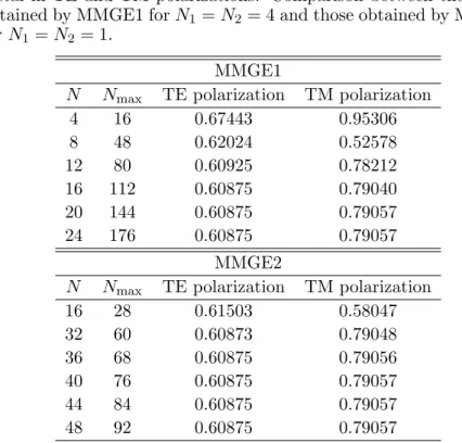
Table 1. Minus-first order reflected efficiency R−1of highly conductive

metal in TE and TM polarizations. Comparison between the results obtained by MMGE1 for N1 = N2 = 4 and those obtained by MMGE2

for N1 = N2 = 1.

MMGE1

N N_max TE polarization TM polarization

4 16 0.67443 0.95306 8 48 0.62024 0.52578 12 80 0.60925 0.78212 16 112 0.60875 0.79040 20 144 0.60875 0.79057 24 176 0.60875 0.79057 MMGE2

N Nmax TE polarization TM polarization

16 28 0.61503 0.58047 32 60 0.60873 0.79048 36 68 0.60875 0.79056 40 76 0.60875 0.79057 44 84 0.60875 0.79057 48 92 0.60875 0.79057

MMGE1 without subdivisions. This can be a serious drawback since the eigenvalue problem is the most time consuming step in the MMGE approach. The current version of the MMGE (MMGE2) removes this disadvantage. The results obtained by the MMGE2 are presented in the lower part of the Table 1 and show a remarkable stability. Under TE polarization, the forth digit of R−1 = 0.6087 is stabilized as soon

as N_max reaches 60 while it is necessary to use N_max = 112 in order to have the same result with the MMGE1 (N₁ = N₂ = 4). Under TM polarization, the same behavior is observed on R₋₁ = 0.7905 as soon as Nmaxreaches 76; while it is necessary to use Nmax= 144 with

the MMGE1. Thus with the new implementation of the MMGE one not only gains in stability but lowers the computational cost by using smaller matrices.

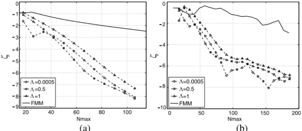
In order to highlight how striking the improvement of convergence brought by the MMGE is, we present in Figures 3(a) and 3(b) a comparison between the results obtained by the Fourier Modal Method and MMGE2 for three arbitrary values of Λ: Λ = 0.0005, 0.5 and 1.

20 40 60 80 100 9 8 7 6 5 4 3 2 1 0 Nmax =0.0005 =0.5 =1 FMM 0 50 100 150 200 10 8 6 4 2 0 Nmax =0.0005 =0.5 =1 FMM -ζ ζ Λ Λ Λ Λ Λ Λ (a) (b)

Figure 3. Minus-first order reflected efficiency of highly conductive metal obtained by MMGE2 in (a) TE and (b) TM polarizations. Comparison with Fourier modal method.

For that purpose, we introduced the error function:

ζ(Nmax) = log10| 1 −

R−1(Nmax−

P_NΩ

i=1Ni)

R−1(Nmax) |, (44)

that measures the relative variation of the efficiency.

After this discussion on the stability, let us turn to the study of the influence of the parameter Λ in the MMGE2 implementation. It is of fundamental importance to notice that this parameter acts through the weighting function w(ξ), also known as the density function, by introducing the measure (1 − ξ2)Λ−1/2dξ in the integral of the inner

product. The density increases or decreases in the vicinity of ξ = ±1 depending on the value of Λ. When Λ is close to zero, it is easy to see that the density increases around ξ = ±1; and in this case Gegenbauer polynomials are similar to Chebychev ones. The particular case of Λ = 0.5, which, corresponds to Legendre polynomials, involves an equipartition on the interval [−1, 1]. This density decreases around

ξ = ±1 when Λ is greater than 0.5. All this, is from a theoretical

point of view. In practice, it is reasonable to think, that for a given grating problem at least one optimal value of Λ may exist that allows describing the field at best. Indeed if we look to Tables 2 and 3, we find that the convergence is slightly improved in the case of TM polarization for Λ = 0.45 while Λ = 0.5 seems to be the best value in the case of TE polarization.

Other numerical investigations (not reported here) concerning the filling factor, the dielectric permittivity and the angle of incidence did not allow us to draw a general rule about the choice of Λ. All we can

0 0.1 0.2 0.3 0.4 0.5 0 0.1 0.2 0.3 0.4 0.5 0.6 0.7 0.8 0.9 1 groove width ( m)

minus first order efficiency

µ

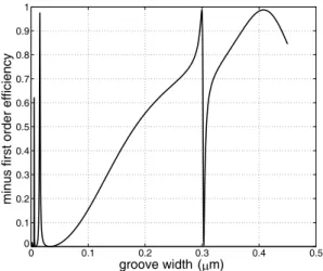
Figure 4. Minus-first order reflected efficiency of a metallic lamellar grating with respect to the groove width in TM polarization. Numerical parameters: θ = 30◦_{, ν}

3 = ν22 = 10i, ν1 = ν21 = 1,

d = h = 0.5 µm, λ = 0.6328 µm, Nmax= 20.

Table 2. Minus-first order reflected efficiency obtained by MMGE2 of highly conductive metal in TE polarization. Influence of the parameter Λ in the convergence of the results.

TE polarization Nmax N Λ = 5e − 4 Λ = 0.15 Λ = 0.25 Λ = 0.45 Λ = 0.5 50 27 0.60854 0.60858 0.60863 0.60877 0.60882 54 29 0.60865 0.60866 0.60868 0.60875 0.60877 58 31 0.60870 0.60871 0.60871 0.60874 0.60875 62 33 0.60873 0.60873 0.60873 0.60874 0.60875 66 35 0.60874 0.60874 0.60874 0.60874 0.60875 70 37 0.60874 0.60874 0.60874 0.60874 0.60875 74 39 0.60874 0.60874 0.60874 0.60874 0.60875 78 41 0.60874 0.60874 0.60874 0.60875 0.60875 82 43 0.60874 0.60874 0.60874 0.60875 0.60875 86 45 0.60874 0.60874 0.60874 0.60875 0.60875 90 47 0.60875 0.60875 0.60875 0.60875 0.60875 94 49 0.60875 0.60875 0.60875 0.60875 0.60875

Table 3. Minus-first order reflected efficiency obtained by MMGE2 of highly conductive metal in TM polarization. Influence of the parameter Λ in the convergence of the results.

TM polarization Nmax N Λ = 5e − 4 Λ = 0.15 Λ = 0.25 Λ = 0.45 Λ = 0.5 50 27 0.79273 0.79229 7.9178 0.79023 0.78972 54 29 0.79164 0.79149 7.9128 0.79054 0.79028 58 31 0.79107 0.79102 7.9094 0.79060 0.79048 62 33 0.79079 0.79078 7.9075 0.79060 0.79054 66 35 0.79067 0.79067 7.9065 0.79059 0.79056 70 37 0.79061 0.79061 7.9061 0.79058 0.79057 74 39 0.79059 0.79059 7.9059 0.79058 0.79057 78 41 0.79058 0.79058 7.9058 0.79058 0.79057 82 43 0.79058 0.79058 7.9058 0.79058 0.79057 86 45 0.79058 0.79058 7.9058 0.79058 0.79057 90 47 0.79058 0.79058 7.9058 0.79058 0.79058 94 49 0.79058 0.79058 7.9058 0.79058 0.79058 assert is that the extreme values of the interval [0, 0.5] are far from being the optimal in certain cases.

Finally, we test the stability of our approach over a grating configuration that posed numerical problems to the FMM [13] and for which solutions have been proposed by some authors [14, 15]. It consists of a grating with a relative dielectric permittivity equal to

−100 and all the other parameters are given in Figure 4.

The minus-first reflected order is drawn versus the groove width. It is remarkable to see that this curve is obtained by Nmaxas small as

20 without any instability. 6. CONCLUSION

In the present work, the modal method by Gegenbauer polynomials expansions has been improved by getting rid of undesirable instabilities. These ones have been shown to be directly linked to the computation of the Gegenbauer polynomials through a series sum. The introduction of a suitable weighting function in the inner product gives an additional degree of freedom that allows for stable and efficient evaluation of this latter. Thus the current version of the MMGE is very stable, accurate and converges very rapidly. It clearly extends the domain of action of modal methods with outstanding performances.

APPENDIX A. AN EXAMPLE OF THE MATRICES CONSTRUCTION IN THE CASE OF TWO MEDIA Ω₁ AND Ω₂

For the both media, the resolution of the wave equation leads to: " LΩ1 [N −2]×[N ] 0 0 LΩ2 [N −2]×[N ] # " aΩ1 [1 : N ],p aΩ2 [1 : N ],p # = β_p2 " GΩ1 [N −2]×[N ] 0 0 GΩ2 [N −2]×[N ] # " aΩ1 [1 : N ],p aΩ2 [1 : N ],p # . (A1)

By using the boundary conditions of Eqs. (4), (5) and (6), the expansion coefficients of highest orders aΩ1

(N −1),p, aΩN,p1 , aΩ(N −1),p2 and

aΩ2

N,pare expressed in terms of the coefficients of lower orders. For that

purpose let us set:

TΩi [n](x0, κ) = κ      h bΩi [n](x0) i " dbΩi [n] dx # x0     . (A2)

Eqs. (4), (5) and (6) lead to  a Ω1 [N −1,N ],p aΩ2 [N −1,N ],p   = T  a Ω1 [1 : N −2],p aΩ2 [1 : N −2],p   , (A3)

where the matrix T is defined as follows: T = −  T Ω1 [N −1,N ](0, 1) − TΩ[N −1,N ]2 (0, 1) TΩ1 [N −1,N ](f d − d, τ ) − T Ω2 [N −1,N ](f d, 1)   −1  T Ω1 [1 : N −2](0, 1) − TΩ[1 : N −2]2 (0, 1) TΩ1 [1 : N −2](f d − d, τ ) − TΩ[1 : N −2]2 (f d, 1)   . (A4)

τ = eik sin θd _{is the pseudo-periodic factor and f denoted the}

filling factor of the lamellar grating. Therefore the vector h aΩ1 [1 : N ],p, a Ω2 [1 : N ],p i_t

of Eq. (A1) can be expressed in term of the vector

h aΩ1

[1 : N −2],p, aΩ[1 : N −2],p2

i_t

with the following matrix relation: " aΩ1 [1 : N ],p aΩ2 [1 : N ],p # = C " aΩ1 [1 : N −2],p aΩ2 [1 : N −2],p # . (A5)

The matrix C can be written in the following concise form: C = · C₁₁ C₁₂ C21 C22 ¸ . (A6)

The matrices Cii of N × (N − 2) size, describe the coupling between

higher and lower coefficients of a same subinterval namely C11 in the

subinterval Ω1 and C22in Ω2: C11 =          1 0 . . . 0 0 1 . .. 0 .. . . . . . .. ... 0 0 . . . 1 T_1,1 T_1,2 . . . T_{1,N −2} T2,1 T2,2 . . . T2,N −2          , (A7) C₂₂ =          1 0 . . . 0 0 1 . .. 0 .. . . . . . .. ... 0 0 . . . 1 T3,N −2+1 T3,N −2+2 . . . T3,2(N −2) T4,N −2+1 T4,N −2+2 . . . T4,2(N −2)          , (A8)

whereas Cij, i 6= j of N × (N − 2) size take onto account the

interconnection between the subintervals:

C12 =          0 0 . . . 0 0 0 . .. 0 .. . . . . . .. ... 0 0 . . . 0 T1,N −2+1 T1,N −2+2 . . . T1,2(N −2) T2,N −2+1 T2,N −2+2 . . . T2,2(N −2)          , (A9) C21 =          0 0 . . . 0 0 0 . .. 0 .. . . . . . .. ... 0 0 . . . 0 T_3,1 T_3,2 . . . T_{3,N −2} T4,1 T4,2 . . . T4,N −2          . (A10)

It is easy to show that " GΩ1 [N −2]×[N ] 0 0 GΩ2 [N −2]×[N ] # · C11 C12 C21 C22 ¸ = " GΩ1 [N −2]×[N −2] 0 0 GΩ2 [N −2]×[N −2] # , (A11)

consequently, Eq. (A1) is written as follows: " LΩ1 [N −2]×[N ] 0 0 LΩ2 [N −2]×[N ] # · C11 C12 C21 C22 ¸ "aΩ1 [1 : N −2],p aΩ2 [1 : N −2],p # = β_p2 " GΩ1 [N −2]×[N −2] 0 0 GΩ2 [N −2]×[N −2] # " aΩ1 [1 : N −2],p aΩ2 [1 : N −2],p # . (A12)

Finally in the case of two media, we are led to the compu-tation of the eigenvalues β2

p and their associated eigenvectors

h aΩ1

[1 : N −2],p, aΩ[1 : N −2],p2

i_t

of a matrix with dimension Nmax= (2(N −

2)) × (2(N − 2)). REFERENCES

1. Botten, I. C., M. S. Craig, R. C. McPhedran, J. L. Adams, and J. R. Andrewartha, “The dielectric lamellar diffraction grating,”

Optica Acta, Vol. 28, 413–428, 1981.

2. Botten, I. C., M. S. Craig, R. C. McPhedran, J. L. Adams, and J. R. Andrewartha, “The finitely conducting lamellar diffraction grating,” Optica Acta, Vol. 28, 1087–1102, 1981.

3. Knop, K., “Rigorous diffraction theory for transmission phase gratings with deep rectangular grooves,” J. Opt. Soc. Am., Vol. 68, 1206–1210, 1978.

4. Li, L., “New formulation of the fourier modal method for crossed surface-relief gratings,” J. Opt. Soc. Am., Vol. 14, 2758–2767, 1997.

5. Morf, R. H., “Exponentially convergent and numerically efficient solution of Maxwell’s equations for lamellar gratings,” J. Opt. Soc.

Am. A, Vol. 12, 1043–1056, 1995.

6. Plumey, J. P., B. Guizal, and J. Chandezon, “Coordinate transformation method as applied to asymmetric gratings with vertical facets,” J. Opt. Soc. Am. A, Vol. 14, 610–617, 1997.

7. Edee, K., P. Schiavone, and G. Granet, “Analysis of defect in E.U.V. lithography mask using a modal method by nodal B-spline expansion,” Japanese Journal of Applied Physics, Vol. 44, No. 9A, 6458–6462, 2005.

8. Armeanu, A. M., M. K. Edee, G. Granet, and P. Schiavone, “Modal method based on spline expansion for the electromagnetic analysis of the lamellar grating,” Progress In Electromagnetics

Research, Vol. 106, 243–261, 2010.

9. Harrington, R. F., Field Computation by Moment Methods, The Macmillan Company, New York, 1968, reprinted by IEEE Press, New York, 1993.

10. Edee, K., “Modal method based on subsectional Gegenbauer polynomial expansion for lamellar gratings,” J. Opt. Soc. Am., Vol. 28, 2006–2013, 2011.

11. Hochstrasser, U. W., “Orthogonal polynomials,” Handbook of

Mathematical Functions, 771–802, M. Abramowitz and I. A.

Stegun, eds., Dover, 1965.

12. Yala, H., B. Guizal, and D. Felbacq, “Fourier modal method with spatial adaptive resolution for structures comprising homogeneous layers,” J. Opt. Soc. Am. A, Vol. 26, 2567–2570, 2009.

13. Popov, E., B. Chernov, M. Nevi`ere, and N. Bonod, “Differential theory: Application to highly conducting gratings,” J. Opt. Soc.

Am. A, Vol. 21, 199–206, 2004.

14. Lyndin, N. M., O. Parriaux, and A. V. Tishchenko, “Modal analysis and suppression of the Fourier modal method instabilities in highly conductive gratings,” J. Opt. Soc. Am. A, Vol. 24, 3781– 3788, 2007.

15. Guizal, B., H. Yala, and D. Felbacq, “Reformulation of the eigenvalue problem in the Fourier modal method with spatial adaptive resolution,” Opt. Lett. A, Vol. 34, 2790–2792, 2009.