HAL Id: hal-01408944
https://hal.archives-ouvertes.fr/hal-01408944
Preprint submitted on 5 Dec 2016
HAL is a multi-disciplinary open access
archive for the deposit and dissemination of
sci-entific research documents, whether they are
pub-lished or not. The documents may come from
teaching and research institutions in France or
abroad, or from public or private research centers.
L’archive ouverte pluridisciplinaire HAL, est
destinée au dépôt et à la diffusion de documents
scientifiques de niveau recherche, publiés ou non,
émanant des établissements d’enseignement et de
recherche français ou étrangers, des laboratoires
publics ou privés.
Parameter Free Piecewise Dynamic Time Warping for
time series classification
Vanel Steve Siyou Fotso, Engelbert Mephu Nguifo, Philippe Vaslin
To cite this version:
Vanel Steve Siyou Fotso, Engelbert Mephu Nguifo, Philippe Vaslin. Parameter Free Piecewise Dynamic
Time Warping for time series classification. 2016. �hal-01408944�
Parameter Free Piecewise Dynamic Time Warping for time series classification
Vanel Steve SIYOU FOTSO
∗†Engelbert MEPHU NGUIFO
∗†Philippe VASLIN
∗†Abstract
Several improvements have been done in time series clas-sification over the last decade. One of the best solutions is to use the Nearest Neighbour algorithm with Dynamic Time Warping(DTW), as the distance measure. Computing DTW is relatively expensive especially with very large time series. Piecewise Dynamic Time Warping (PDTW) is an efficient variant which consists of segmenting time series into fixed-length segments. However, the choice of the optimal size (or number) of segments remains a difficult challenge for end users. The Brute-force solution, a naive solution, repeats the classification with each segment size, and selects the one with the best accuracy. This solution is not appropriated especially when dealing with massive and large time series data. In this work, we propose a parameter free approach for PDTW, that finds the size (or number) of segments to be used with the Nearest Neighbour algorithm. Our approach is a heuristic that is parameter free since it does not require any domain specific tuning. Several properties of our heuris-tic are studied, and an extensive experimental comparison demonstrates its efficiency and effectiveness, in terms of ac-curacy and runtime.
1 Introduction
Time series are ubiquitous in sciences as for example in economics [6], in medicine [7], in finance [18] or in computer science [20]. An important task is time series comparison that can be done in two main ways. Ei-ther the comparison method considers that Ei-there is no time distortion as in Euclidian distance (ED), or it con-siders that some small time distortions exist between time axis of time series as in Dynamic Time Warping alignment algorithm (DTW) [28]. Since time distortion often exists between time series, DTW often has better results than the ED [3]. An exhaustive comparison of time series algorithms [1] shows that DTW is among the efficient techniques to be used. However, DTW has two major drawbacks: the comparison of two time series un-der DTW is time-consuming [21] and DTW sometimes produces pathological alignments [14]. A pathological alignment occurs when, during the comparison of two
∗Clermont Auvergne University, Blaise Pascal University,
LIMOS, BP 10448, F-63000 CLERMONT-FERRAND, FRANCE
†CNRS, UMR 6158, LIMOS, F-63178 AUBIERE, FRANCE
time series X and Y , one datapoint of the time series X is compared to a large subsequence of datapoints of Y . A pathological alignment causes a wrong comparison.
Three categories of methods are used to avoid pathological alignments with DTW:
• The first one adds constraints to DTW [22], [27], [2], [23], [10]. The main idea here is to limit the length of the subsequence of a time series that can be compared to a single datapoint of another time series.
• The second one suggests to skip datapoints that produce pathological alignment during the compar-ison of two time series [17], [9], [19].
• The third one proposes to replace the datapoints of time series by a high level abstraction that captures the local behavior of those time series. A high-level abstraction can be a histogram of values that captures the repartition of time series datapoints in space [28], or a feature that captures the local properties of time series, such as the trend with Derivative DTW (DDTW) [14] or the mean with Piecewise DTW (PDTW) [13].
PDTW has been introduced with the aim to speed up the computation of DTW, which depends on the length of the time series. PDTW suggests to use a compact abstraction of time series instead of the raw data. Indeed, PDTW proposes to split a time series into consecutive fixed-length segments and to compute the mean of each segment. Then, the mean is used instead of the data points in the segment to compare the time series.
In practice, a straightforward way to use PDTW is the brute-force approach that consists in exploring all the possible values for the number of segments. How-ever, this is not feasible with long time series data. So, the question is how to automatically fix this parameter without a considerable decrease of classification accu-racy ?
In this paper, we propose a parameter free heuristic to align piecewise aggregate time series with DTW that approximates the optimal value of the number of segments to be considered during the alignment. In
this heuristic, the number of segments is chosen based on the quality of the alignment, which is evaluated by the classification error on the training set. The best classification algorithm to use for this purpose is one Nearest Neighbor (1NN) that is combined with PDTW. In this case 1NN is the best because its classification error directly depends on the alignment of time series, since it has no other parameters [26].
2 Background and related work
Definition 2.1. A time series X = x1, · · · , xn is a
sequence of numerical values representing the evolution of a specific quantity during the time. xn is the most
recent value.
2.1 Dynamic Time Warping algorithm. DTW [12] is a time series alignment algorithm that performs a non-linear alignment while minimizing the distance between two time series. To align two time series :
X = x1, x2, · · · , xn;
Y = y1, y2, · · · , ym.
the algorithm constructs an n × m matrix where the cell (i, j) of the matrix corresponds to the squared distance (xi − yj)2 that is the alignment between xi
and yj. To find the best alignment between two
time series, it constructs the path that minimizes the sum of squared distances. This path, noted W = w1, w2, . . . , wk, . . . , wK, should respect the following
constraints:
• Boundary constraint: w1= (1, 1) and wK= (n, m)
• Monotonicity constraint: Given wk = (i, j),
wk+1= (i0, j0) then i ≤ i0 and j ≤ j0
• Continuity constraint: Given wk = (i, j), wk+1 =
(i0, j0) then i0 ≤ i + 1 and j0 ≤ j + 1
The warping path is computed by using an algorithm based on the dynamic programming paradigm that solves the following recurrence:
γ(i, j) = d(xi, yj)+min{γ(i−1, j−1), γ(i−1, j), γ(i, j−1)},
where d(xi, yj) is the squared distance contained in
the cell (i, j) and γ(i, j) is the cumulative distance at the position (i, j) that is computed by the sum of the squared distance at the position (i, j) and the minimal cumulative distance of its three adjacent cells.
Definition 2.2. A segment Xi of length l of the time
series X of length n (l < n) is a sequence constituted by l variables of X starting at the position i and ending at the position i + l − 1. We have: Xi= xi, xi+1, ..., xi+l−1
Definition 2.3. The arithmetic average of the data points of a segment Xi of length l is noted ¯Xi and is
defined by: ¯ Xi= 1 l l−1 X j=0 xi+j
Definition 2.4. Let T be the set of time series. The Piecewise Aggregate Approximation (PAA) is defined as follows: P AA : T × N∗→ T (X, N ) 7→ P AA(X, N ) = ( ¯ X1, · · · , ¯XNif N < |X| X otherwise Piecewise Dynamic Time Warping Algorithm (PDTW) [13] is the DTW algorithm applied on Piece-wise Aggregate time series [11]. Let N ∈ N∗, X and Y be two time series.
P DT W (X, Y, N ) = DT W (P AA(X, N ), P AA(Y, N )). The number of segments N that one considers greatly influences the quality of the alignment of the time series. However, PDTW does not give any information on the way to choose it. To do so, [4] proposes the Iterative Deepening Dynamic Time Warping Algorithm (IDDTW).
2.2 Iterative Deepening Dynamic Time Warp-ing. IDDTW only considers values for the number of segments that are power of 2 and for each value, com-putes an error distribution by comparing PDTW with the standard DTW at each level of compression. It takes as input: the query Q, the dataset D, the user’s confi-dence (or tolerance for false dismissals) user conf , and the set of standard deviations StdDev obtained from the error distribution.
• The algorithm starts with applying the classic DTW to the first K candidates from the dataset. The results of the best matches to the query are contained in R, with |R| = K. The best so f ar is determined from argmaxR.
• Both the query Q and each subsequent candidate C are approximated using PAA representations with N segments to determine the corresponding PDTW.
• A test is performed to determine whether the can-didate C can be pruned off or not. If the result of the test is found to have a probability that it could
be a better match than the current best so f ar, a higher resolution of the approximation is required. Then each segment of the candidate is split into two segments to obtain a new candidate.
• The process of approximating Q and C to deter-mine the PDTW should be reapplied and the test is repeated for all levels of approximations until they fail the test or their true distance DTW is deter-mined.
Doing so, IDDTW finds the number of segments that best approximates DTW and speeds up its compu-tation. However, the goal of IDDTW is not the same as ours, which is to find the number of segments that best aligns the time series and speeds-up the computation of DTW. Actually, IDDTW has three main drawbacks:
• It only considers the numbers of segments for PDTW that are power of 2;
• It requires a user-specified tolerance for false dis-missals that influences the quality of the approxi-mation, but the algorithm does not give any indi-cation on how to choose the tolerance;
• It considers DTW as a reference while looking for the number of segments that best aligns the time series. However, because of pathological alignments, DTW sometimes fails to align time series properly.
In this paper, we propose a heuristic named param-eter Free piecewise DTW (FDTW) that deals with all the drawbacks of IDDTW: it considers all the possible values for the number of segments, it is parameter-free and it finds a number of segments for PDTW based on the quality of the time series alignment namely the clas-sification error. The next section presents a definition of our heuristic.
3 Heuristic search of the number of segments 3.1 Problem definition. Let D = {di} be a set
of datasets composed of time series. We note |di| the
number of time series of the dataset di.
Let X ∈ dibe a time series of the dataset di; we note
|X| = n the length of the time series X. For simplicity of notation we suppose that all the time series of dihave
the same length. Definition 3.1.
1N N DT W : D → [0, 1] di7→ 1N N DT W (di)
1N N DT W (di) is the classification error of one Nearest
Neighbour with Dynamic Time Warping on the dataset di.
Definition 3.2. Let d ⊆ T be a subset of time series, N ∈ N∗, P AAset(d, N ) = {P AA(X, N ), ∀X ∈ d}
Definition 3.3.
1N N P DT W : D × {1 . . . n} → [0, 1] (di, N ) 7→ 1N N P DT W (di, N ) =
= 1N N DT W ◦ P AAset(di, N )
1N N P DT W (di, N ) is the classification error of
1-NN with PDTW using N segments on di.
Our goal is to find the number of segments that allows P DT W to best align time series. P DT W gives a good alignment when its classification error with 1N N is low [21]. Our problem is then to find the number of segments N that minimizes 1N N P DT W (di, N ).
Formaly, given a dataset di, we look for the
number of segments N ∈ {1 . . . n} such that 1N N P DT W (di, N ) = min
1≤α≤n{1N N P DT W (di, α)}.
3.2 Brute-force search. The simplest way to find the value for the number of segments that minimized the classification error is to test all the possible values. Obviously, this method is time consuming as we have to test n values to find the one that has the minimal classification error. The time complexity of this process is : O((|trainingset| 2 ) 2× X N ∈C N2), |C| = n, where C is the set of values for the number of segments.
To reduce the time of the search, the heuristic proposes to look for the number of segments with the minimal classification error without testing all the possible values.
3.3 Parameter free heuristic. The idea of our heuristic is the following:
1. We choose Nc candidates distributed in the
space of possible values to ensure that we are going to have small, medium and large values as candidates. The candidates values are: n, n−jNn
c k , n−2×jNn c k , ..., n− Nc× j n Nc k
. For instance, if the length of time series is n = 12 and the number of candidates is Nc= 4, we are
going to select the candidates 12, 9, 6, 3. 1, 2,[3], 4, 5,[6], 7, 8,[9], 10, 11,[12]
2. We evaluate the classification error with 1N N P DT W for each candidate that we have previously chosen and we select the candidate that has the mini-mal classification error: it is the best candidate. In our example, we may suppose that we get the minimal value with the candidate 6 it is thus the best candidate at this step.
1, 2, 3, 4, 5,[6], 7, 8, 9, 10, 11, 12
3. We respectively look between the predecessor (i.e., 3 here) and successor (i.e., 9 here) of the best can-didate for a number of segments with a lower classifica-tion error. This number of segments corresponds to a local minimum. In our example, we are going to test the values 4, 5, 7 and 8 to see if there is a local minimum.
4. We restart at step one, while choosing differents candidates during each iteration to ensure that we return a good local minimum. We fix the number of iterations to blog(n)c. At each iteration the first candidate is n − (number of iteration − 1).
In short, in the worst case, we test the Nc first
candidates to find the best one. Then, we test 2nN
c
other candidates to find the local minimum. We finally perform nb(Nc) = Nc + 2nNc tests. The number of tests
that we have to perform is a function of the number of candidates. How many candidates should we consider to reduce the number of tests? The first derivative of the function nb vanishes when Nc =
√
2n and the second derivative is positive so the minimal number of tests is done when the number of candidates Nc =
√ 2n. Algorithm 1 presents the details of the heuristic.
Time complexity: We use the training set to find the number of segments that should be considered with PDTW. To do so, we applied 1N N on the training set that costs
O((|trainingset| 2 ) 2× X N ∈C N2), |C| = log(n)−1 X i=0 8√n − i.
where (|trainingset|2 )2 comes from 1N N algorithm
and P
N ∈C
N2comes from P DT W with N being one value of the number of segments, and C being the set of values for the number of segments. At each iteration, the heuristic tests nb(√2n) = 8√n number of segments. We have log(n) iterations so |C| =
log(n)−1
P
i=0
8√n − i
Lemma 3.1. For a given a dataset di F DT W (di) ≤
1N N DT W (di). The quality of the alignment of our
heuristic is better than that of DTW.
Proof. 1N N DT W (di) = 1N N P DT W (di, n).
1N N DT W (di) is then one of the candidate
con-sidered by the heurisitic F DT W . Since F DT W
returns the minimal classification error from all candi-dates, the classification error of 1N N DT W is always greater than or equal to F DT W .
Algorithm 1 FDTW(training set, test set, n, nb rep=log(n))
# Look for a good value of the number of segments N
# using the training set for (i in 0 : (nb rep − 1)) do
tab N ← 1 : (n − i) l ← f loor(n/sqrt(2 ∗ n))
tab N candidats ← seq(f rom = n, to = 1, by = −l)
# Parallel execution of 1NNPDTW mat r ← 1N N P DT W (training set, tab N candidats)
# Mark candidates already used to not reuse for (i in tab candidats) do
tab N [i] ← −1 end for
# Search for the best candidate with the minimal error
min ← minimun(mat r)
# look for the local minimun near of the best candidate
result[[(i + 1)]] ← localM inimun(min.N min, min.error min, training set, tab N )
end for
# The best local minimal error m ← minimun(result)
return m
A heuristic does not always give the optimal value. To ensure that it gives a result not far from the optimal value, one approach is to guarantee that the result of the heuristic always lies in an interval with respect to the optimal value [8].
In our case, we are looking for the number of segments that allows a good alignment of time series. The alignment is good when the classification error with 1NN is minimal or when the accuracy is maximal.
Let di be a dataset: accmax(di) = 1 −
min
1≤α≤n{1N N P DT W (di, α)} is the maximal accuracy
for the dataset di, accDT W = 1 − 1N N DT W (di) is
the accuracy with di and 1NNDTW and accF DT W =
To ensure the quality of our heuristic FDTW, Proposition 3.1 assume that 1N N DT W is better than the baseline classifier Zero Rule. Zero rule classifier is a simple classifier that predicts the majority class of test data (if nominal) or average value (if numeric). Zero rule is often used as baseline classifier [5]. The minimal value of the accuracy of Zero rule is 1c where c is the number of classes of the dataset.
Proposition 3.1. For a given dataset di that has ci
classes, ci∈ N∗,
if accDT W ≥ c1i then
1
ci × accmax ≤ accF DT W ≤
accmax
Proof. By definition, accF DT W ≤ accmax We look for
k ∈ N such that k1× accmax≤ accF DT W
1
k × accmax≤ accF DT W
i.e. accmax accF DT W ≤ k or accmax accF DT W ≤ 1 accF DT W
because accmax≤ 1 and
1 accF DT W
≤ 1 accDT W
because accDT W ≤ accF DT W
1 accDT W ≤ ci because 1 ci ≤ accDT Wby hypotesis We take k = ci
4 Experiments and discussion
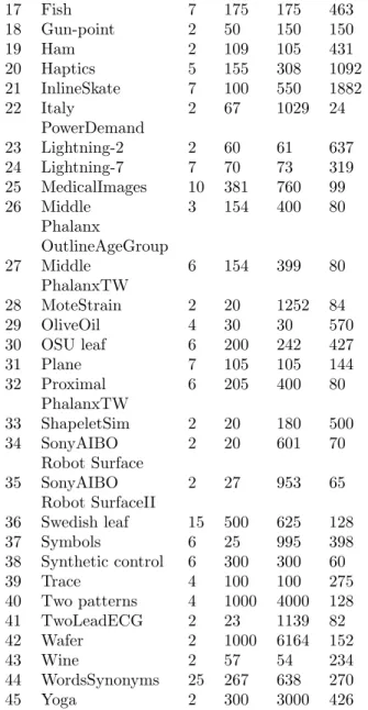
4.1 Datasets. The performance of FDTW has been tested on 45 datasets of the UCR time series datamining archive [3], which provides a large collection of datasets that cover various domains (Table 1). Each dataset is divided into a training set and a testing set. The 45 datasets possess between 2 and 50 classes, the length of the time series varies from 24 to 1882, the training sets contain between 20 and 1000 time series and the testing sets contain between 28 and 6164 time series. An implementation of BF, IDDTW and FDTW is available online [24]
4.2 Results. Firstly, to evaluate the quality of our heuristic FDTW, we compared its classification errors with that of IDDTW (Figure 4) and the minimal one (Figure 3). The classification error was calculated based on the holdout model evaluation and the minimal one was find by applying Brute-force search (BF) on both training set and testing set. FDTW and IDDTW used the training set to find the number of segments N using 3 fold cross validation. IDDTW tested all the values of N that were equal to a power of two and kept the one that had a minimum classification error. We also compared FDTW to BF and IDDTW in terms of number of tested values (Figure 1), running time (Figure 2) and compression ratio.
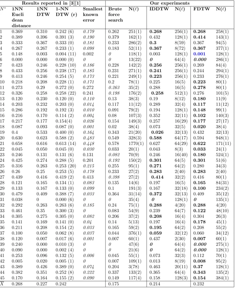
Then, we compared FDTW to other classification methods reported in the literature. The comparison was based on the classification error calculated using the hold out evaluation model. The smallest classification error reported on each dataset and the 1NN classifica-tion error of Euclidean distance, DTW without a warp-ing window and DTW with best warpwarp-ing window have been published by previous researchers [3] [1]. In this paper we report the 1NN classification error of Brute-force search, IDDTW and FDTW.
N◦ Dataset clas Size Size Time ses of of se
trai tes ries ning ting len set set gth 1 50Words 50 450 455 270 2 Adiac 37 390 391 176 3 Beef 5 30 30 470 4 Car 4 60 60 577 5 CBF 3 30 900 128 6 Coffee 2 28 28 286 7 Cricket X 12 390 390 300 8 Cricket Y 12 390 390 300 9 Cricket Z 12 390 390 300 10 Distal 3 139 400 80 Phalanx OutlineAge Group 11 Distal 6 139 400 80 Phalanx TW 12 Earthquakes 2 139 322 512 13 ECG 2 100 100 96 14 ECGFiveDays 2 23 861 136 15 Face (all) 14 560 1690 131 16 Face (four) 4 24 88 350
17 Fish 7 175 175 463 18 Gun-point 2 50 150 150 19 Ham 2 109 105 431 20 Haptics 5 155 308 1092 21 InlineSkate 7 100 550 1882 22 Italy 2 67 1029 24 PowerDemand 23 Lightning-2 2 60 61 637 24 Lightning-7 7 70 73 319 25 MedicalImages 10 381 760 99 26 Middle 3 154 400 80 Phalanx OutlineAgeGroup 27 Middle 6 154 399 80 PhalanxTW 28 MoteStrain 2 20 1252 84 29 OliveOil 4 30 30 570 30 OSU leaf 6 200 242 427 31 Plane 7 105 105 144 32 Proximal 6 205 400 80 PhalanxTW 33 ShapeletSim 2 20 180 500 34 SonyAIBO 2 20 601 70 Robot Surface 35 SonyAIBO 2 27 953 65 Robot SurfaceII 36 Swedish leaf 15 500 625 128 37 Symbols 6 25 995 398 38 Synthetic control 6 300 300 60 39 Trace 4 100 100 275 40 Two patterns 4 1000 4000 128 41 TwoLeadECG 2 23 1139 82 42 Wafer 2 1000 6164 152 43 Wine 2 57 54 234 44 WordsSynonyms 25 267 638 270 45 Yoga 2 300 3000 426
Table 1: Detailed information about the datasets 4.3 Discussions. Comparing FDTW and BF ap-proaches (Figure 1) clearly shows that the number of candidates in BF is considerably reduced in FDTW by a factor at least greater than 2.5. This number is expo-nentially correlated to the time series length, for exam-ple FDTW tested 0.08% less candidates than BF with the dataset ItalyPowerDemand that has the shortest time series length of our sample (24 data points) and 76% less candidates than BF with dataset Inlineskate that has the longest time series of our sample (1882 data points). Actually, the number of candidates to be tested ranges from 1 to n, n being the length of time series. This demonstrates an advantage of FDTW in terms of space exploration and thus indirectly in terms of
mem-ory usage and execution time. However, FDTW tested more candidates than IDDTW, which tested in average 96% less candidates than Brute-force search (Figure 1).
Figure 1: Comparison of the number of tested values of the parameter, number of segments with the Brute-force search algorithm, FDTW and IDDTW. x-axis datasets are sorted according to the length of the time series.
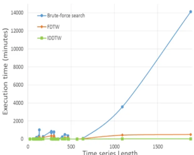
Nevertheless, the values of the number of segments are evaluated on the training set. To take into account the cost of classification performed on the testing set, we also compare the methods FDTW, IDDTW and Brute-force search based on their execution time on the training and the testing sets.
Generally, FDTW is 8 times faster than Brute-force search with an average execution time of 176 minutes against 1386 minutes for Brute-force search. IDDTW is 7 times faster than FDTW and remains the fastest with an average execution time of 24 minutes. The execution time increases with the length of the time series (Figure 2). The increase of Brute-force search execution time is faster than that of FDTW and IDDTW. This can be seen on the dataset Lightning-2 whose time series have a length equal to 637 data points.
As regard in the compression ratio, the heuristic uses a compact representation for time series whose length contains in average 44% data points less than the initial time series against 63% for IDDTW.
The experiments show that IDDTW is faster and test fewer candidates. However, FDTW have better performance. Actually, FDTW resulted in a lower classification error than IDDTW on 22 datasets and the same classification error than IDDTW on 8 datasets (Figure 4). They also show that the classification error of Brute-force search (BF) is smaller than the smallest classification error reported in the literature on six datasets and is equal to the smallest classification error
Figure 2: Comparison of the execution time of the Brute-force search algorithm, FDTW and IDDTW.
reported on four datasets. Moreover, In average, BF is better than the other algorithms of Table 4.3 with a classification error of 0.175. In other words, it is a good strategy to piecewise aggregate time series before classifying them if we know a good number of segment to use.
Our heuristic FDTW managed to find the minimum error for 9 datasets (Coffee, ECGFiveDays, Gun-point, ItalyPowerDemand, OliveOil, Plane, Synthetic control, Trace, Two patterns). It also outperforms the smallest classification error reported in the literature on dataset CBF (N◦5). The methods of the literature are
Figure 3: Comparison of the classification error of the Brute-force search algorithm in x-axis and FDTW in y-axis.
1NN associated with Euclidiean distance, DTW without warping windows, DTW with warping windows. FDTW outperforms 1NN associated with Euclidiean distance
Figure 4: Comparison of the classification error of IDDTW in x-axis and FDTW in y-axis. The points below the diagonal represent the datasets for which FDTW is better than IDDTW.
ED on 33, they are equal on 1 dataset. FDTW outperforms 1NN associated with DTW on 19 datasets, they are equal on 11 datasets. FDTW outperforms 1NN associated with DTW with warping windows on 19 datasets they are equal on 2 datasets.
5 Conclusion
Our problem was to choose a good number of seg-ments for Piecewise Dynamic Time Warping. To an-swer this question, we proposed a heuristic approach called Parameter Free Piecewise Dynamic Time Warp-ing (FDTW) that proposes an approximation of the best number of segments to be used during times series classi-fication based on DTW. FDTW has been experimented on 45 data sets on a classification task. In average, it returned a classification error lower than the one of ID-DTW. Our approach is a heuristic that is parameter free since it does not require any domain specific tun-ing. This work allows to reduce the storage space and the processing time of time series classification without decreasing the quality of the alignment. As a perspec-tive, we plan to use piecewise aggregate time series with other variants of DTW to improve the classification. Us-ing the same strategy presented in FDTW, we plan to find the number of segments to be considered for sym-bolic representations of time series like SAX [15], ESAX [16], SAX-TD [25].
References
[1] A. Bagnall, E. Keogh, J. Lines, A. Bostrom, and J. Large, Time
Se-Results reported in [3][1] Our experiments
N◦ 1NN 1NN 1-NN Smallest Brute N(`) IDDTW N(`) FDTW N(`) Eucli DTW DTW (r) known force
dean error search distance 1 0.369 0.310 0.242 (6) 0.179 0.262 251(1) 0.268 256(1) 0.268 258(1) 2 0.389 0.396 0.391 (3) 0.190 0.379 162(1) 0.432 128(1) 0.414 143(1) 3 0.333 0.367 0.333 (0) 0.181 0.233 286(2) 0.3 8(59) 0.367 94(5) 4 0.267 0.267 0.233 (1) 0.098 0.183 52(11) 0.367 8(72) 0.367 377(1) 5 0.148 0.003 0.004 (11) 0.002 0 118(1) 0.003 128(1) 0.001 128(1) 6 0.000 0.000 0.000 (0) 0 0 13(22) 0 64(4) 0.000 286(1) 7 0.423 0.246 0.228 (10) 0.186 0.228 142(2) 0.256 256(1) 0.269 84(4) 8 0.433 0.256 0.238 (17) 0.185 0.231 271(1) 0.241 256(1) 0.244 294(1) 9 0.413 0.246 0.254 (5) 0.173 0.221 249(1) 0.223 256(1) 0.233 276(1) 10 0.218 0.208 0.228 (1) 0.171 0.2 78(1) 0.225 16(5) 0.223 80(1) 11 0.273 0.29 0.272 (0) 0.272 0.263 35(2) 0.288 16(5) 0.278 80(1) 12 0.326 0.258 0.258 (22) 0.241 0.198 176(2) 0.258 512(1) 0.276 101(5) 13 0.120 0.230 0.120 (0) 0.110 0.13 38(3) 0.19 8(12) 0.180 11(9) 14 0.203 0.232 0.203 (0) 0.014 0.117 11(12) 0.289 32(4) 0.117 11(12) 15 0.286 0.192 0.192 (3) 0.010 0.091 79(2) 0.194 128(1) 0.148 99(1) 16 0.216 0.170 0.114 (2) 0.004 0.08 107(3) 0.352 32(11) 0.102 140(3) 17 0.217 0.177 0.154(4) 0.026 0.154 149(3) 0.257 16(29) 0.177 27(17) 18 0.087 0.093 0.087 (0) 0.001 0.02 38(4) 0.073 32(5) 0.020 38(4) 19 0.4 0.533 0.400 (0) 0.164 0.343 21(20) 0.026 32(13) 0.432 32(13) 20 0.630 0.623 0.588 (2) 0.483 0.549 328(3) 0.588 64(17) 0.594 948(1) 21 0.658 0.616 0.613 (14) 0.448 0.578 1770(1) 0.627 64(29) 0.622 171(11) 22 0.045 0.050 0.045 (0) 0.030 0.033 20(1) 0.043 8(3) 0.033 24(1) 23 0.246 0.131 0.131 (6) 0.131 0.082 70(9) 0.246 16(40) 0.180 524(1) 24 0.425 0.274 0.288 (5) 0.201 0.192 150(2) 0.301 64(5) 0.301 51(6) 25 0.316 0.263 0.253 (20) 0.215 0.255 95(1) 0.271 64(2) 0.280 34(3) 26 0.26 0.25 0.253 (5) 0.178 0.233 27(2) 0.283 2(40) 0.283 2(40) 27 0.439 0.416 0.419 (2) 0.413 0.398 27(2) 0.414 32(2) 0.416 80(1) 28 0.121 0.165 0.134 (1) 0.083 0.135 14(6) 0.197 16(5) 0.165 84(31) 29 0.133 0.167 0.133 (0) 0.099 0.1 191(3) 0.167 32(18) 0.100 234(2) 30 0.479 0.409 0.388 (7) 0.033 0.364 31(14) 0.372 32(13) 0.409 35(12) 31 0.038 0 0.000 (6) 0 0 35(4) 0 128(1) 0 135(1) 32 0.292 0.263 0.263 (6) 0.185 0.24 75(1) 0.288 4(20) 0.288 4(20) 33 0.461 0.35 0.300 (3) 0 0.083 54(9) 0.239 64(7) 0.122 48(10) 34 0.305 0.275 0.305 (0) 0.082 0.206 37(2) 0.208 16(4) 0.304 26(3) 35 0.141 0.169 0.141 (0) 0.04 0.14 5(13) 0.197 16(4) 0.178 45(1) 36 0.211 0.208 0.154 (2) 0.033 0.165 59(2) 0.195 64(2) 0.208 55(2) 37 0.100 0.050 0.062 (8) 0.037 0.044 376(1) 0.059 32(12) 0.060 34(12) 38 0.120 0.007 0.017 (6) 0.001 0.007 60(1) 0.437 2(30) 0.007 60(1) 39 0.240 0.000 0.010 (3) 0 0 47(6) 0 64(4) 0.000 275(1) 40 0.090 0.000 0.002 (4) 0 0 21(6) 0 64(2) 0.000 128(1) 41 0.253 0.096 0.132 (5) 0.006 0.045 55(1) 0.073 32(3) 0.112 70(1) 42 0.005 0.020 0.005 (1) 0 0.007 109(1) 0.013 8(19) 0.008 95(2) 43 0.389 0.426 0.389 (0) 0.074 0.204 3(78) 0.463 20(11) 0.37 128(1) 44 0.382 0.351 0.252 (8) 0.222 0.337 133(2) 0.365 64(4) 0.343 135(2) 45 0.170 0.164 0.155 (2) 0.090 0.149 117(4) 0.158 128(3) 0.154 384(1) X 0.268 0.227 0.242 0.175 0.214 0.232
Table 2: Comparison of classification errors. In italics, the smallest classification error. In bold, the smallest classification error between IDDTW and FDTW. N is the number of segments selected and ` is the number of data points in a segment which is equal to bNnc.
ries Classification Website, October 2016. http://www.timeseriesclassification.com/index.php. [2] K. S. Candan, R. Rossini, X. Wang, and M. L.
Sapino, sdtw: computing dtw distances using locally relevant constraints based on salient feature alignments, Proceedings of the VLDB Endowment, 5 (2012), pp. 1519–1530.
[3] Y. Chen, E. Keogh, B. Hu, N. Begum, A. Bagnall, A. Mueen, and G. Batista, The ucr time series classification archive, July 2015. www.cs.ucr.edu/ eamonn/time series data/.
[4] S. Chu, E. J. Keogh, D. M. Hart, M. J. Pazzani, et al., Iterative deepening dynamic time warping for time series., in SDM, SIAM, 2002, pp. 195–212. [5] J. Cuˇr´ın, P. Fleury, J. Kleindienst, and
R. Kessl, Meeting state recognition from visual and aural labels, in International Workshop on Machine Learning for Multimodal Interaction, Springer, 2007, pp. 24–25.
[6] J. Hamilton, A new approach to the economic analysis of nonstationary time series and the business cycle, Econometrica: Journal of the Econometric Society, 57 (1989), pp. 357–384.
[7] B. Huang and W. Kinsner, Ecg frame classification using dynamic time warping, Electrical and Computer Engineering,, 2 (2002), pp. 1105–1110.
[8] O. H. Ibarra and C. E. Kim, Fast approximation al-gorithms for the knapsack and sum of subset problems, Journal of the ACM (JACM), 22 (1975), pp. 463–468. [9] F. Itakura, Minimum prediction residual principle applied to speech recognition, IEEE Transactions on Acoustics, Speech, and Signal Processing, 23 (1975), pp. 67–72.
[10] Y.-S. Jeong, M. K. Jeong, and O. A. Omitaomu, Weighted dynamic time warping for time series classifi-cation, Pattern Recognition, 44 (2011), pp. 2231–2240. [11] E. Keogh, K. Chakrabarti, M. Pazzani, and S. Mehrotra, Dimensionality Reduction for Fast Similarity Search in Large Time Series Databases, Knowledge and Information Systems, 3 (2001), pp. 263–286.
[12] E. Keogh and C. A. Ratanamahatana, Exact in-dexing of dynamic time warping, Knowledge and In-formation Systems, 7 (2004), pp. 358–386.
[13] E. J. Keogh and M. J. Pazzani, Scaling up dynamic time warping for datamining applications, in Proceed-ings of the sixth ACM SIGKDD international confer-ence on Knowledge discovery and data mining, ACM, 2000, pp. 285–289.
[14] E. J. Keogh and M. J. Pazzani, Derivative dynamic time warping, Proceedings of the 1st SIAM Interna-tional Conference on Data Mining, (2001), pp. 1–11. [15] J. Lin, E. Keogh, S. Lonardi, and B. Chiu, A
sym-bolic representation of time series, with implications for streaming algorithms, in Proceedings of the 8th ACM SIGMOD workshop on Research issues in data mining and knowledge discovery, ACM, 2003, pp. 2–11. [16] B. Lkhagva, Y. Suzuki, and K. Kawagoe, Extended
sax: Extension of symbolic aggregate approximation for financial time series data representation, DEWS2006 4A-i8, 7 (2006).
[17] J. Longin, M. Vasilis, W. Qiang, L. Rolf, A. Chotirat, and E. Keogh, Elastic partial match-ing of time series, in 9th European Conference On Principles And Practice Of Knowledge Discovery In Databases, Porto, Portugal, 2005.
[18] A. Marszalek and T. Burczynski, Modeling and forecasting financial time series with ordered fuzzy can-dlesticks, Information Sciences, 273 (2014), pp. 144– 155.
[19] C. Myers, L. Rabiner, and A. Rosenberg, Perfor-mance tradeoffs in dynamic time warping algorithms for isolated word recognition, IEEE Transactions on Acoustics, Speech, and Signal Processing, 28 (1980), pp. 623–635.
[20] C. Myers, L. R. Rabiner, and A. E. Rosenberg, Performance tradeoffs in dynamic time warping algo-rithms for isolated word recognition, IEEE Transac-tions on Acoustics, Speech, and Signal Processing, 28 (1980), pp. 623–635.
[21] T. Rakthanmanon, B. Campana, A. Mueen, G. Batista, B. Westover, Q. Zhu, J. Zakaria, and E. Keogh, Searching and mining trillions of time series subsequences under dynamic time warping, Pro-ceedings of the 18th ACM SIGKDD, (2012), pp. 262– 270.
[22] C. A. Ratanamahatana and E. Keogh, Mak-ing Time-series Classification More Accurate UsMak-ing Learned Constraints, 2004, pp. 11–22.
[23] H. Sakoe and S. Chiba, Dynamic programming algo-rithm optimization for spoken word recognition, IEEE Transactions on Acoustics, Speech and Signal Process-ing, 26 (1978), pp. 43–49.
[24] V. S. Siyou Fotso, E. Mephu Nguifo, and P. Vaslin, Source code of FDTW, October 2016. https://github.com/VanelS/FDTW.
[25] Y. Sun, J. Li, J. Liu, B. Sun, and C. Chow, An improvement of symbolic aggregate approximation distance measure for time series, Neurocomputing, 138 (2014), pp. 189–198.
[26] X. Wang, A. Mueen, H. Ding, G. Trajcevski, P. Scheuermann, and E. Keogh, Experimental com-parison of representation methods and distance mea-sures for time series data, Data Mining and Knowledge Discovery, 26 (2013), pp. 275–309.
[27] D. Yu, X. Yu, Q. Hu, J. Liu, and A. Wu, Dynamic time warping constraint learning for large margin near-est neighbor classification, Information Sciences, 181 (2011), pp. 2787–2796.
[28] Z. Zhang, P. Tang, and R. Duan, Dynamic time warping under pointwise shape context, Information Sciences, 315 (2015), pp. 88–101.