HAL Id: hal-00808577
https://hal.archives-ouvertes.fr/hal-00808577
Submitted on 5 Apr 2013
HAL is a multi-disciplinary open access
archive for the deposit and dissemination of
sci-entific research documents, whether they are
pub-lished or not. The documents may come from
teaching and research institutions in France or
abroad, or from public or private research centers.
L’archive ouverte pluridisciplinaire HAL, est
destinée au dépôt et à la diffusion de documents
scientifiques de niveau recherche, publiés ou non,
émanant des établissements d’enseignement et de
recherche français ou étrangers, des laboratoires
publics ou privés.
Estimating rock fall frequency in a limestone cliff using
LIDAR measurements
Antoine Guerin, Jean-Pierre Rossetti, Didier Hantz, Michel Jaboyedoff
To cite this version:
Antoine Guerin, Jean-Pierre Rossetti, Didier Hantz, Michel Jaboyedoff. Estimating rock fall frequency
in a limestone cliff using LIDAR measurements. First International Conference on Landslides Risk,
Mar 2013, Tabarka, Tunisia. p. 293-301. �hal-00808577�
Estimating rock fall frequency in a limestone cliff using
LIDAR measurements
Antoine Guerin
1, Jean-Pierre Rossetti
1, Didier Hantz
1, Michel Jaboyedoff
21Institut des Sciences de la Terre, Université Joseph Fourier, CNRS, Grenoble, France
2Centre de Recherche sur l'Environnement Terrestre, Université de Lausanne, Switzerland
Abstract. Terrestrial Laser Scanner has been used to detect rock falls which have occurred in a
limestone cliff during some years, in the difficult configuration of the Subalpine Chains. In a rock wall of width 750 m and height 200 m, 130 rock falls larger than 0.1 m3 have been detected for a period of 1180 days.
The distribution of the rock fall volumes is well fitted by a power law, with an exponent which is compatible with the exponent found for the 120 km long cliffs of the Grenoble area. But the spatial-temporal frequencies given by the two analyses are very different. The number of rock falls larger than 1 m3, which occur per century and per hm2, is about 150 times larger for the bedded limestone of Sequanian stage than for the massive limestones of Tithonian and Barremian stages.
Keywords: rock fall, frequency, hazard, risk, LiDAR, terrestrial laser scanner.
1 Introduction
Estimating rock fall frequency is needed to characterize a diffuse rock fall hazard
(Picarelli et al., 2005; Fell et al., 2005; Hantz, 2011). Up to now this frequency is determined from historical inventories. The minimal volume detected in these inventories can be relatively small when the rock blocks fall on a road or railway from a cut slope, but it is larger when they fall from a high rock cliff (Dussauge et al., 2002). In the last years, terrestrial laser scanner (TLS) has been used to detect rock falls in coastal cliffs (Rosser et al., 2005 ; Dewez et al., 2009) and in high mountain walls (Ravanel et al., 2011), where the rock fall frequency is relatively high. We have used this method to detect rock falls in a limestone cliff of the Subalpine Ranges, which threatens the Grenoble town.
2 Description of the cliff and measurements
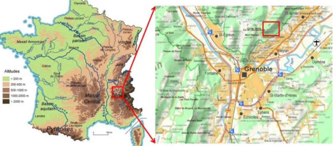
The Mont Saint-Eynard (1308 m) is located 4 km to the North of the Grenoble centre and towers above a residential area of the town (Figures 1 and 2). Its South-East face consists of, from top to bottom: a 120 m high limestone cliff (Tithonian and upper Kimmeridgian stages); a 100 m high forested slope of marl and marly limestone (Kimmeridgian stage); a 240 m high limestone cliff (Sequanian stage); a 300 m high forested talus slope, covering marl and marly limestone of the Orfordian stage. This paper describes the results obtained for the Sequanian cliff.
The measurement place was located at the foot of the talus slope, on a protection embankment at an elevation of 580 m. The inclined distance to the cliffs ranges between 625 m and 900 m. Note that no place was found closer to the cliffs. Photographs and laser measurements were carried out in August 2009 and November 2012.
The laser scanner technology also called LiDAR (Light Detection And Ranging), is based on the acquisition of a point cloud using a time-of-flight distance measurement of an infrared laser pulse which reflects on the topography. The raw data consist of the x, y, z coordinates of each reflection point and the intensity of the reflected pulse. The y axis corresponds to the outward axis of the LiDAR camera and x and z axes are parallel to the sides of the LiDAR scene (x is roughly horizontal).
Figure 1. Localisation of the Mont Saint-Eynard.
We have used two Optech systems: ILRIS-3D in 2009 and ILRIS-LR in 2012. The main characteristics of these systems are given in Table 1. It can be seen that ILRIS-LR has a higher repetition rate, allowing a greater number of points to be measured for a given period of time.
Parameter ILRIS-3D ILRIS-LR
Range 80% reflectivity 1200 m 3000 m Range 10% reflectivity 400 m 1330 m
Minimum range 3 m 3 m
Laser repetition rate 2500 to 3500 Hz 10 000 Hz
Efficiency 100 % 100 %
Raw range accuracy 7 mm @ 100 m 7 mm @ 100 m Raw angular accuracy 8 mm @ 100 m 8 mm @ 100 m
Field of view 40° x 40° 40° x 40° Minimum step size 0,001146° (20 µrad) 0,001146° (20 µrad)
Maximum density 2 cm @ 1000 m 2 cm @ 1000 m Rotational speed 0,001 to 20°/sec 0,001 to 20°/sec Beam diameter 22 mm @ 100 m 27 mm @ 100 m Beam divergence 0,009740° (170 µrad) 0,014324° (250 µrad) Laser wavelength 1535 nm 1064 nm Integrated camera 3,1 MP 3,1 MP
3
The point spacing was about 20-30 cm in 2009 and about 10-13 cm in 2012. According to the distances given above and the accuracy given in Table 1, the expected accuracy of our measurements ranges from about 5 cm for the closest points to 7,5 cm for the farthest ones. Two scans were taken to cover a cliff width of about 750 m.
3 Data analysis
The softwares 3DReshaper Application and Cloud Compare has been used to process the point clouds.
3.1. Cleaning the raw point cloud
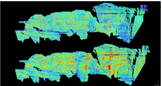
Vegetation has a lower reflectance than the rock making up the cliff. Thus, a reflectance threshold has been chosen to remove most of the points corresponding to vegetation. After cleaning, the two point clouds consisted of 1.5 Mpt (left scene) and 1.2 Mpt (right scene) in 2009 and 7.1 (left) and 5.8 Mpt (right) in 2012. They are shown in Figure 2. The average distance between the points was 21-29 cm in 2009 and 10-13 cm in 2012.
Figure 2. Point clouds measured in 2009 (high) and 2012 (low).
3.2. Georeferencing
Georeferencing the LiDAR point clouds was made by registering these with a DEM (1 m x 1 m) using Lambert 2 extended (x,y) coordinates and NGF IGN 69 leveling. The DEM is shown in Figure 3. Then the coordinate system has been changed in order to easily determine the width and the thickness of the fallen compartments. The width is defined horizontally, parallel to the cliff (x direction), the thickness is defined horizontally, perpendicular to the cliff direction (y direction) and the height is parallel to the z axis. The positive direction is inside the cliff for the y axis and towards the East side for the x axis.
Figure 3. Digital Elevation Model used for georeferencing.
3.3. Meshing the 2012 point clouds
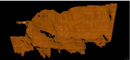
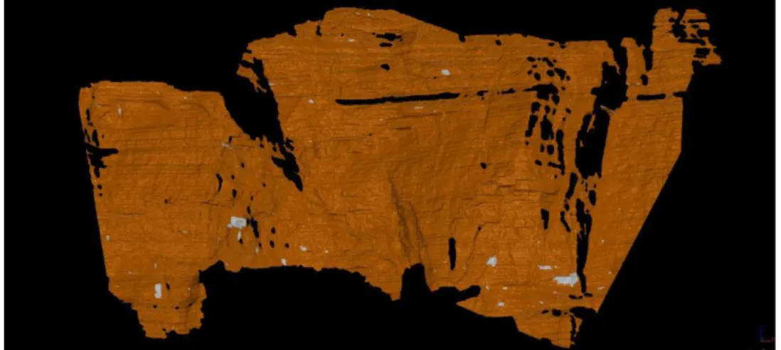
The more recent point clouds (2012) have been transformed in two meshes (polyhedrons), made up of 1.6 million (left scene) and 1.1 million (right scene) of triangles (Figures 4). The average distances between the vertex of the polyhedrons are respectively 26 cm and 36 cm, and the vertex numbers 800 000 and 570 000. Note that these numbers are about ten times less than the initial numbers of points of the clouds. This reduction is associated to the noise reduction process we used in 3DReshaper and is also necessary for numerical reasons. Registration of the 2012 point cloud with the corresponding mesh allows estimating the roughness of the rock surface at the scale of the triangles making up the mesh. It appears that about 50 % of the points are closer than 1 cm from the mesh, 90 % are closer than 3 cm and 99 % are closer than 7 cm. Note that, in the later case, most of the deviations larger than 7 cm are located on vegetation areas.
5
Figure 4b. Mesh for the right scene 2012 and rock fall detected.
3.4. Registration of the point clouds
As georeferencing with the DEM was not precise enough, the 2012 meshes and the point clouds acquired in 2009 have been registered (fitted) together in order to put them in the same coordinate system. Ideally, the deviations between these objects should be due only to rock falls occurred between 2009 and 2012. But in reality, there are other causes of deviations: (a) measurement accuracy; (b) the 2009 measurement points do not correspond to the 2012 ones and are not exactly on the triangles defined by the 2012 vertex (due to the curvature and the roughness of the rock surface); (c) the later cause is accentuated in areas where the triangles are large (this situation occurs particularly near the limits of the mesh); (d) vegetation element which has not been removed; (e) earth slide due to the impact of an overlying rock fall.
3.5. Detection of the rock falls
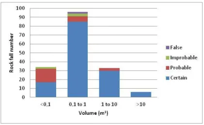
A rock fall is considered certain when a positive deviation is observed and the comparison of the 2009 and 2012 photos shows that a rock fall has occurred between these dates. Such a comparison is shown in Figure 5. When a positive deviation is observed and the comparison of the 2009 and 2012 photos shows that no rock fall has occurred, the deviation is considered to be a false rock fall. False rock falls are due to the conditions (c) or (d) expressed in the later paragraph. When a positive deviation is observed and the photo comparison can't conclude if a rock fall has occurred or not, the deviation is considered to be an improbable rock fall if the conditions (c) or (d) occur or a probable rock fall if these conditions don't occur. This situation occurs more and more when the extent of the deviation zone decreases. The reason is that small rock falls are difficult to observe on photographs. Figure 6 shows the proportions of certain, probable, improbable and false rock falls as a function of the rock fall volume.
Figure 5. Rock fall proven by comparison of 2009 and 2012 photographs (81 m3).
Figure 6. Proportions of certain, probable, improbable and false rock falls as a function of the rock
fall volume.
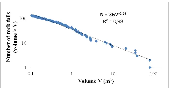
3.6. Size-frequency relation
Figure 7 shows the cumulative distribution of the rock fall volumes larger than 0.1 m3. It appears that the distribution is well fitted by a power law:
b
aV
N
(1)with V, rock fall volume, N, number of rock falls larger than V, b = 0,65 and a = 36. The constant a represents the number of rock falls larger than 1 m3, observed between August 27, 2009, and November 19, 2012.
4. Discussion
Hantz et al. (2003) analyzed the cumulative distribution of rock fall volumes between 102 and 107 m3, occurred in the 120 km long limestone cliffs of the Grenoble area, which include the Mont Saint-Eynard cliff. They found that a power law well describes the
7
distribution, with an exponent absolute value of 0.55 ± 0.11. The values obtained for the Grenoble area and for the Mont Saint-Eynard appear to be compatible with a value of 0.6 ± 0.11. Concerning the spatial-temporal rock fall frequency, the number of rock falls larger than 1 m3, which occur per century and per hm2, is about 75 for the Mont Saint-Eynard and 0,5 for the Grenoble area. These frequencies correspond to different rock masses. The cliffs of the Grenoble area consist mainly of massive limestone of Tithonian and Barremian stages, whereas the studied cliff consists of bedded limestone of Sequanian stage. Although the latter is included in the Grenoble area cliffs, it represents a tiny part of it.
Figure 7. Cumulative distribution of the rock fall volumes.
5. Conclusion
Terrestrial Laser Scanner can be used to detect rock falls which have occurred in high rock walls during some years, in the difficult configuration of Subalpine Chains. In a rock wall of width 750 m and height 200 m, 130 rock falls larger than 0.1 m3 have been detected for a period of 1180 days. The distribution of the rock fall volumes is well fitted by a power law, with an exponent (b = 0.65) which is compatible with the exponent found for the 120 km long cliffs of the Grenoble area (b = 0.55 ± 0.11). But the spatial-temporal frequencies given by the two analyses are very different. The number of rock falls larger than 1 m3, which occur per century and per hm2, is about 150 times larger for the bedded limestone of Sequanian stage than for the massive limestone of Tithonian and Barremian stages.
References
Dewez T., Chamblas G., Lasseur E., and Vandromme R. (2009) Five seasons of chalk cliff face erosion monitored by terrestrial laser scanner: from quantitative description to rock fall probabilistic hazard assessment. Geophysical Research Abstracts, 11, 2009-8218.
Dussauge-Peisser C, Helmstetter A, Grasso J-R, Hantz D, Jeannin M, Giraud A. (2002) Probabilistic approach to rock fall hazard assessment: potential of historical data analysis. Natural
Hazards and Earth System Sciences, 2: 15-26.
Fell R., Ho K.K.S., Lacasse S., Leroi E. (2005) A framework for landslide risk assessment and management. In: Landslide Risk Management, Hungr, Fell, Couture & Eberhardt (eds), Taylor & Francis Group, London, 3-25.
Hantz D., Vengeon J.M., Dussauge-Peisser C. (2003) An historical, geomechanical and probabilistic approach to rock-fall hazard assessment. Natural Hazards and Earth System Sciences, 3: 693-701.
Hantz D. (2011) Quantitative assessment of diffuse rock fall hazard along a cliff foot. Natural
Hazards and Earth System Sciences, 11: 1303–1309.
Picarelli L., Oboni F., Evans S.G., Mostyn G., Fell R. (2005) Hazard characterization and quantification. In: Landslide Risk Management, Hungr, Fell, Couture & Eberhardt (eds), Taylor & Francis Group, London, 27-61.
Ravanel L., Deline P., Jaillet S. (2011) Quatre années de suivi de la morphodynamique des parois rocheuses du massif du Mont Blanc par laserscanning terrestre. Images et modèles 3D en
milieux naturels (2011) 69-76.
Rosser N.J., Petley D.N., Lim M., Dunning S.A., and Allison, R.J (2005) Terrestrial laser scanning for monitoring the process of hard rock coastal cliff erosion. Quarterly Journal of