Détection et suivi multi-objets dans des séquences vidéo

(1)

HAL Id: tel-02177037

https://tel.archives-ouvertes.fr/tel-02177037

Submitted on 8 Jul 2019

HAL is a multi-disciplinary open access archive for the deposit and dissemination of sci-entific research documents, whether they are pub-lished or not. The documents may come from teaching and research institutions in France or abroad, or from public or private research centers.

L’archive ouverte pluridisciplinaire HAL, est destinée au dépôt et à la diffusion de documents scientifiques de niveau recherche, publiés ou non, émanant des établissements d’enseignement et de recherche français ou étrangers, des laboratoires publics ou privés.

Ala Mhalla

To cite this version:

Ala Mhalla. Multi-object detection and tracking in video sequences. Computer Vision and Pattern Recognition [cs.CV]. Université du Centre (Sousse, Tunisie), 2018. English. �NNT : 2018CLFAC084�. �tel-02177037�

(2)

UNIVERSITY of Clermont Auvergne - Clermont Ferrand

EDSPI DOCTORAL SCHOOL

P H D T H E S I S

to obtain the title of

DOCTOR OF THE UNIVERSITY

of Clermont Auvergne University - Clermont-France

Speciality : Computer Science

Defended by

Ala Mhalla

Multi-object Detection and Tracking in Video

Sequences

Defended on 4 Avril 2018

Jury :

Reviewer: _{M. Christophe Garcia} - LIRIS laboratory

Reviewer: _{M. Adel Alimi} - REGIM laboratory

Examiner _{M. Christophe Ducottet} - Hubert Curian laboratory Co-director: _{Mme. Najoua Essoukri ben Amara - LATIS laboratory}

Co-director: _{M.Thierry Chateau} - Institut Pascal laboratry Co-supervisor: _{M. Sami Gazzah} - LATIS laboratory

(3)

(4)

Abstract:

The work developed in this PhD thesis is focused on video sequence analysis. The latter consists of object detection, categorization and tracking. The development of reliable solutions for the analysis of video sequences opens new horizons for several applications such as intelligent transport systems, video surveillance and robotics.

In this thesis, we put forward several contributions to deal with the problems of detecting and tracking multi-objects on video sequences. The proposed frameworks are based on deep learning networks and transfer learning approaches.

In a first contribution, we tackle the problem of multi-object detection by putting forward a new transfer learning framework based on the formalism and the theory of a Sequential Monte Carlo (SMC) filter to automatically specialize a Deep Con-volutional Neural Network (DCNN) detector towards a target scene. The suggested specialization framework is used in order to transfer the knowledge from the source and the target domain to the target scene and to estimate the unknown target distri-bution as a specialized dataset composed of samples from the target domain. These samples are selected according to the importance of their weights which reflects the likelihood that they belong to the target distribution. The obtained special-ized dataset allows training a specialspecial-ized DCNN detector to a target scene without human intervention.

In a second contribution, we propose an original multi-object tracking frame-work based on spatio-temporal strategies (interlacing/inverse interlacing) and an interlaced deep detector, which improves the performances of tracking-by-detection algorithms and helps to track objects in complex videos (occlusion, intersection, strong motion).

In a third contribution, we provide an embedded system for traffic surveillance, which integrates an extension of the SMC framework so as to improve the detection accuracy in both day and night conditions and to specialize any DCNN detector for both mobile and stationary cameras.

Throughout this report, we provide both quantitative and qualitative results. On several aspects related to video sequence analysis, this work outperforms the state-of-the-art detection and tracking frameworks. In addition, we have successfully implemented our frameworks in an embedded hardware platform for road traffic safety and monitoring.

Keywords:

Artificial intelligence, Computer vision, Transfer learning, Deep learning, Multi-object detection, Specialization, Tracking-by-detection, Multi-Multi-object tracking, Em-bedded system.

(5)

(6)

List of Figures

1.1 Some applications of the work carried out in this thesis. . . 2

1.2 Main challenges of object detection . . . 3

1.3 Outline of the manuscript . . . 7

2.1 Examples of object detection . . . 10

2.2 Some challenges on object detection . . . 11

2.3 Classical diagram of object detection by sliding window . . . 12

2.4 Illustration of selective search . . . 14

2.5 Analogy between the human brain and neural networks . . . 15

2.6 Classical schema of supervised learning for object classification . . . 17

2.7 Interest of neural networks. . . 18

2.8 Artificial neuron . . . 19

2.9 An example of an MLP . . . 20

2.10 Examples of convolution filters . . . 20

2.11 A convolutional network for the recognition of handwritten digits . . 21

2.12 Convolution illustration . . . 22

2.13 Illustration of Max Pooling . . . 23

2.14 Examples of activation function . . . 23

2.15 Error rate of different architectures on ImageNet for object classification 24 2.16 Illustration of AlexNet architecture . . . 25

2.17 VGG architecture . . . 25

2.18 residual connection . . . 26

2.19 ResNet architecture. . . 26

2.20 Differences between traditional learning and transfer learning . . . . 28

2.21 Transfer learning advantages. . . 29

2.22 Different types of transfer learning . . . 29

2.23 Illustrated transfer of examples . . . 32

2.24 Example of feature transfer . . . 34

2.25 Transfer method of Aytar and Zisserman . . . 36

3.1 General synoptic of the proposed framework . . . 42

3.2 Block diagram of proposed approach . . . 45

3.3 The foreground algorithm result. . . 49

3.4 Description of training strategy . . . 51

3.5 Annotation errors . . . 54

3.6 ROC curves for several public and private datasets and with different annotations . . . 57

3.7 ROC curves for convergence of specialization process . . . 58

(9)

4.1 General synoptic of the proposed framework . . . 67

4.2 Interlacing step . . . 68

4.3 Examples of interlaced strategies . . . 69

4.4 Estimation of bounding boxes by interpolation strategy . . . 70

4.5 Building an annotated interlaced video . . . 71

4.6 Image examples of evaluated datasets. . . 72

4.7 Comparison between proposed interlaced MOT framework and base-line one . . . 75

4.8 Frame skipping strategy with four different sets of parameters for interlaced model . . . 76

4.9 Output examples of interlaced specialized object detector for four interlacing strategies . . . 78

4.10 Examples of FRCNN-MHT failures (with interlacing strategy (D=2, s=6, g=3)) . . . 79

5.1 Main challenges on traffic applications . . . 82

5.2 General synoptic of specialization framework . . . 83

5.3 Architecture of the suggested MF R-CNN deep detector . . . 89

5.4 Block diagram of proposed approach . . . 91

5.5 Description of tracklet steps . . . 92

5.6 Illustration of how compute weights . . . 93

5.7 Improvement of our proposed specialization framework in detecting small-sized objects . . . 97

5.8 ROC curves for comparison between generic Faster R-CNN detector and proposed MF R-CNN one . . . 98

5.9 Efficiency of proposed likelihood function . . . 99

5.10 Image of hardware components of proposed embedded system . . . . 101

6.1 Synoptic diagram of suggested automatic specialization system . . . 106

6.2 Examples of images captured with different type of sensors. . . 107

(10)

List of Tables

2.1 Summary of detection methods by CNN and results on Pascal VOC 2007 [Everingham 2010]. . . 27 2.2 Summarization of different transfer learning approaches applied on

object detection applications. . . 37

3.1 Comparison of detection rate for pedestrian with state of the art (at 0.5 FPPI) . . . 56 3.2 Comparison of detection rate for car with state of the art (at 1 FPPI) 56 3.3 Detection rate for multi-traffic object detection with SMC Faster

R-CNN (at 1 FPPI) . . . 59 3.4 Illustration of similarity matrix between traffic object categories on

Logiroad Traffic dataset . . . 59 3.5 Illustration of similarity matrix between traffic object categories on

MIT Traffic dataset. . . 59 3.6 Description of the difference between the work of Maamatou et al.

[Maâmatou 2016c] and our proposed one. . . 61 4.1 MOTA comparison for several interlacing strategies on several

se-quences of TUD public dataset . . . 74 4.2 Table summarizing results of our framework on PETS and TUD

se-quences . . . 77 4.3 MOTA evaluation metric for several interlacing strategies selected to

produce frame skipping on TUD dataset . . . 78

5.1 Description of the difference between the Faster R-CNN deep neural network architecture and the MF R-CNN one . . . 86 5.2 Description of difference between the SMC Faster R-CNN framework

and proposed approach. . . 87 5.3 Comparison of detection rate for pedestrian with state of art (at 0.5

FPPI) . . . 96 5.4 Comparison of detection rate for car with state of art (at 1 FPPI). . 97 5.5 Comparison of detection rate for Traffic Night dataset with state of

art (at 1 FPPI) . . . 99 5.6 Technical specification details of hardware components . . . 100 5.7 Description of running our specialized detector on the NVIDIA Jetson

TX2 through different deep architectures . . . 100 5.8 Description of running specialized detectors on the NVIDIA platform.101

(11)

(12)

Chapter 1

Introduction

Contents

1.1 Context of the thesis . . . 1

1.2 Problematics . . . 2

1.3 Contributions and organization of the manuscript. . . 3

1.4 Publications. . . 5

One of the many human capacities is the remarkable ability to understand and analyze the environment. From the signals provided by their ocular system, the human being is able to describe the objects that surround them in a very precise and quick way. We can notably emphasize the capacity of the human being to locate and categorize objects while characterizing them by their forms, colors and orientations. One of the many goals of computer vision researchers is to build an intelligent system capable of efficiently analyzing images as human beings. To be reliable, the analysis algorithms must adapt to changes in the appearance of objects related to the context in which they are observed. For example, the appearance of an object may vary depending on the brightness of the environment or it may be partially hidden by another object. This is done by taking into account these constraints, naturally managed by the human brain, which the artificial system must integrate in order to hope to behave like a true intelligent system.

1.1 Context of the thesis

The work done in this PhD project focuses on multi-object detection and tracking, which is based on supervised learning for the automatic analysis of video sequences. Figure1.1illustrates different applications of this work. Detecting and tracking ob-jects remain an important issue because of the number of applications they generate. Among them, we can cite video-surveillance or robotics.

In the context of surveillance for the security of transport infrastructure, the sys-tem must be capable of analyzing and monitoring traffic flows in urban or high-speed areas and collecting statistics, thereby improving safety of road transport. These include video surveillance applications such as monitoring and securing transport infrastructure. We can imagine other video surveillance applications using detec-tion and tracking such as access control, which requires special surveillance and/or high security (metro stations, supermarkets, government institutions, companies, airports, hospitals, research laboratories, etc.).

(13)

Figure 1.1: Various applications of the work carried out in this thesis. Detection and tracking objects in different scenarios. (a) and (b): Object detection in both day and night conditions. (c): Traffic sign detection. (d): Object detection system for an autonomous vehicle. (e) and (f): Multi-object tracking in several conditions.

.

Other types of applications are inherent to the implementation of an analysis system within a vehicle: These are intelligent vehicle applications. These include driver assistance, automatic parking and self-driving. In this context, the detection and the tracking of objects present around the intelligent vehicle is necessary. This predicts the trajectory and speed appropriate to the situation. The constantly evolving performances of these systems will certainly make it possible in the coming years to integrate into the transport infrastructures and the autonomous vehicles of artificial intelligence by vision: a driving system without drivers.

1.2 Problematics

This thesis proposes automatic frameworks for multi-object detection and tracking. In other words, the input of the developed frameworks is a video scene and a generic deep detector and the output is a video containing detected and tracked objects. We have investigated solutions based on transfer learning, deep learning and spatio-temporal strategies to develop our detection and tracking frameworks. The issues addressed are:

(14)

1.3. Contributions and organization of the manuscript 3

• Multi-object detection: It consists in proposing a set of rectangles (bound-ing boxes) contain(bound-ing target objects. This task is necessary to several computer vision applications, in particular in object tracking one. Object detection is a well-studied problem and the main challenges are multiple: occlusion, point of view from which objects are observed, light condition, deformation, intra-class variation, confusion with the background variation, and scale variation (as shown in Figure2.2).

Figure 1.2: Main challenges on object detection (translated from a presentation of Andrew Zisserman, VGG, Oxford) [Simonyan 2014].

• Multi-object tracking: The purpose of tracking is to generate the trajec-tories of objects. Each object has a unique identity assigned to it by the association algorithm. The correspondence between the positions of an ob-ject in successive images constitutes the traob-jectory. In this thesis, we have addressed tracking-by-detection methods which associate successive detection of objects.

• Specialization: Generally, the performance of a generic detector decreases significantly when it is tested on a specific scene due to the large variation between the source training dataset and the target scene. This problem can be solved by specialization. The main idea of specialization is to provide a specialized detector or tracker to a particular scene in order to increase the detection or tracking performances toward a target scene. Specialization is referred to by several terms in the literature such as adaptation, contextuali-sation, etc.

1.3 Contributions and organization of the manuscript

This thesis integrates recent advances in the computer vision domain such as transfer learning and deep learning techniques in order to enhance the detection and the

(15)

tracking performances.

In the past five years, deep learning and transfer learning have been widely used by the computer vision community to solve a lot of tasks. This interest is due to their ability to extract highly relevant information on images, thus allowing the training of high-performance models.

In this respect, deep learning and/or transfer learning seems to be suitable for the construction of multi-object detection and tracking systems. Nevertheless, the very good results of methods using deep learning and/or transfer learning are intimately correlated with the number of data used for their learning.

On the basis of this observation, the general contribution of this thesis is to propose automatic specialization frameworks based on Deep Convolutional Neural Network (DCNN) model, in order to improve the performances of detection and tracking objects in video sequences.

This document is organized as follows. In chapter 2, we present the state-of-the-art in relation with our problematics, namely the deep learning and transfer learning. Object detection is introduced in section 1. Section 2 presents a detailed description of supervised learning as well as deep neural networks used throughout our work. An overview of approaches related to transfer learning is proposed in section 3.

Chapters 3,4 and 5 present the frameworks developed in addition to the proposed contributions.

In chapter 3, we propose a DCNN specialization framework based on a Sequen-tial Monte Carlo (SMC) filter. The idea of this first contribution is to specialize a generic deep detector towards a target scene based on a transductive transfer learning model. The suggested specialization framework leads to improve the per-formance and accuracy of DCNN detectors in each specific scene.

Chapter 4 presents a novel framework for multi-object tracking based on spatio-temporal strategies and an interlaced DCNN detector. The proposed framework makes it possible to improve the tracking performances toward a tracking datasets and to handle the tracking challenges mainly occlusion and intersection.

Chapter 5 presents an applicative contribution: an embedded system for traffic surveillance that can be performed to operate under challenging conditions such as congestion, occlusion and lighting night/day and day/night transitions. This system analyses traffic and particularly focuses on the problem of detecting and categorizing traffic objects on several traffic scenes. Moreover, it contains a robust detector produced by an original specialization framework. The proposed specializa-tion framework presents an extension of the SMC framework menspecializa-tioned in chapter 3.

Finally, chapter 6 represents the conclusion and the perspectives of this research. Figure1.3presents the outline of the manuscript.

(16)

1.4. Publications 5

1.4 Publications

The work presented in this thesis has been the subject of the following publications:

• Journals:

Ala Mhalla, Thierry Chateau, Houda Maâmatou, Sami Gazzah and Najoua Essoukri Ben Amara: "SMC Faster R-CNN: Towards a Scene-Specialized Multi-Object Detector": CVIU journal "Computer Vision and Image Under-standing" Special Issue on Deep Learning for Computer Vision", 2017.(Impact factor 2.5 THOMSON JCR)

Ala Mhalla, Thierry Chateau, Sami Gazzah and Najoua Essoukri Ben Amara: "AN EMBEDDED COMPUTER-VISION SYSTEM FOR MULTI-OBJECT DETECTION IN TRAFFIC SURVEILLANCE", IEEE transaction on intel-ligent transportation system "ITS" 2018. (Impact factor 3.7 THOMSON).

• International Conferences :

Ala Mhalla, Thierry Chateau, Sami Gazzah and Najoua Essoukri Ben Amara: "The Power of Video Interlacing for Deep Learning Based Multi Object Tracking". Submitted to the European Conference on Computer Vision (ECCV 2018).

Ala Mhalla, Thierry Chateau , Sami Gazzah and Najoua Essoukri Ben Amara: "Specialization of a Generic Pedestrian Detector to a Specific Traffic Scene based on Transductive Transfer Learning Method and Deep learning", VISAPP’17: Proceedings of the International Conference on Computer Vision, Imaging and Computer Graphics Theory and Applications (Class C).

Ala Mhalla, Houda Maâmatou, Thierry Chateau, Sami Gazzah and Najoua Essoukri Ben Amara:"Faster R-CNN Scene Specialization with a Sequential Monte-Carlo Framework" in DICTA’16: Proceedings of International Confer-ence on Digital Image Computing: Techniques and Applications (Class B).

Ala Mhalla, Thierry Chateau, Sami Gazzah, Najoua Essoukri Ben Amara: Scene-Specific Pedestrian Detector Using Monte Carlo Framework and Faster R-CNN Deep Model: PhD Forum. Proceedings of the 10th International Conference on Distributed Smart Camera (ICDSC 2016), France, (Class B).

(17)

Sami Gazzah, Ala Mhalla, Najoua Essoukri Ben Amara: Vehicle detection on a video traffic: review and new perpectives. 7th International Conference on Sciences of Electronics, Technologies of Information and Telecommunication, SETIT’17, Hammamet, Tunisia, December 18-20, 2016.

Ala Mhalla, Thierry Chateau, Sami Gazzah, Najoua Essoukri Ben Amara: A Faster R-CNN Multi-Object Detector on a Nvidia Jetson TX1 Embedded Sys-tem: Demo. Proceedings of the 10th International Conference on Distributed Smart Camera, 208-209, Paris/France, September 12-15, 2016 (Class B).

(18)

1.4. Publications 7

SMC Faster R-CNN: Toward a Scene-Specialized Multi-Object

Detector

(Specialization for multi-object detection)

Power of Video Interlacing for Deep-Learning-Based Multi-Object

Tracking

(Specialization for multi-object tracking)

State-of-the-Art

(Machine learning, Deep learning, Transfer learning)

Introduction

An Embedded Computer-Vision System for Multi-Object Detection in

Traffic Surveillance

(Real-time detection for traffic surveillance)

Conclusion & perspectives

Chapter 1

Chapter 2

Chapter 3

Chapter 4

Chapter 5

Chapter 6

(19)

(20)

Chapter 2

State-of-the-Art

Contents

2.1 Introduction . . . 9

2.2 Object detection . . . 10

2.2.1 Detection by sliding window. . . 11

2.2.2 Detection by object proposal . . . 13

2.3 Initiation of deep neural network . . . 15

2.3.1 Supervised learning and neural networks. . . 16

2.3.2 Neural networks: Basic concept . . . 18

2.3.3 Deep convolutional neural networks . . . 20

2.4 Convolutional neural networks for object detection . . . 26

2.5 Transfer learning. . . 27

2.5.1 Motivation of transfer learning . . . 29

2.5.2 Different types of transfer learning . . . 29

2.6 Categorization of transductive transfer learning methods . 31 2.6.1 Transfer of example . . . 31

2.6.2 Model transfer . . . 32

2.6.3 Feature transfer. . . 33

2.7 Transfer learning applications for object detection . . . 35

2.8 Conclusion . . . 36

2.1 Introduction

The aim of this chapter is to present the state-of-the-art and the work in relation with our problematics, namely the deep learning and transfer learning. We have divided this state-of-the-art into several sections. Section 1 refers to the different strategies of object detection. Section 2 presents the Deep Convolutional Neural Networks (DCNN) and reviews the existing work performed in deep neural net-works. After that, a detailed description of transfer learning is provided in section 3. The applications of transfer learning in object detection are described in section 4. Finally, the conclusion of this chapter is given in section 5.

(21)

2.2 Object detection

Object detection is one of the most studied problems in several computer vision applications such as object tracking [Nam 2016][Wang 2016b], semantic segmen-tation [Long 2015][Noh 2015] and object recognition [Huang 2012][Taigman 2014]. The aim of object detection is to find in an input image a set of Regions of Inter-est (RoI) containing target objects. Object detection approaches can be divided into two categories: single-object detection and multi-object detection. The first category focuses on detecting only one type of objects. The detector must be able to decide whether a region of an image corresponds to an object or a back-ground. The second category concentrates on multi-object detection where the detector must be able to predict what type of objects is concerned. There are many public datasets for training and evaluating detectors. We can cite among them Pas-calVOC [Everingham 2010], KITTI [Geiger 2012], MSCOC [Lin 2014] and ILSVRC [Deng 2009]. Figure2.1 illustrates the main objective of object detection.

Figure 2.1: Examples of object detection returned by a multi-object detector. Each bounding box color corresponds to a class of objects. Source [Ren 2015c]

.

Detection challenges: An object detector faces generally several challenges. We quote first the computation time: A robust detector is a detector that should maximize performance while detecting objects as fast as possible. This notion of computation time is particularly important in the design of multi-class detectors because of the number, often very large of object classes to be detected.

The second challenge concerns the variation in object appearances. The latter can vary according to several factors such as: the variation in image resolutions, the size of objects, the points of view under which objects are observed, and light condition.

The third challenge is related to the variation in the appearance of regions that do not correspond to objects (the background). A detector must be able to pre-dict whether a region corresponds to the background even in images resulting from complex environments. Figure 2.2depicts major challenges on object detection.

In the following, we propose more details of the strategies for extracting regions on which the model will be applied. In the next section, we first develop the detection by the sliding window then the detection by object proposals.

(22)

2.2. Object detection 11

Figure 2.2: Detection challenges (translated from a presentation of Ala Mhalla [Mhalla 2016b], DICTA, Australia).

2.2.1 Detection by sliding window

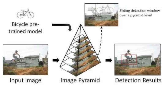
Sliding-window approaches use a previously learnt classification model which con-sists of a 2D window with fixed size permitting the discrimination of the background of objects. The general idea of this type of approaches is to scan the input image using a sliding window. On the other hand, this window goes over the input im-age and produces a confidence score in each imim-age position. In what follows we recall the main steps of the classical sliding window approach based on the pyramid representation (Figure2.3).

• Given an input image, an image pyramid is computed. The computation of this latter consists in resizing an image using several scale factors and several ratios. The set of these images forms the pyramid and each image corresponds to one level. It is necessary to compute a pyramid of images because the sliding window to be applied to the image is of a fixed size. The detection model is generally learnt for a single scale and a single ratio. However, the objects in an image can be of different sizes and have variable ratios. In this way, the objects in the image correspond to the size of the model at least for one level of the pyramid.

• Visual characteristics are extracted on different levels of the pyramid, which makes it possible to obtain a feature map for each pyramidal level.

(23)

Figure 2.3: Classical diagram of object detection by sliding window. A pyramid of images is created from an input image. Visual characteristics are computed. A model is applied in each position and each pyramid level returns candidate boxes. An NMS algorithm is then applied to delete the boxes corresponding to the same object. Source [Suleiman 2017]

• A previously learnt model is applied in each position of the different feature maps, returning a confidence score for each position and each level of the pyramid. This step makes it possible to select candidate boxes (those with the highest confidence scores).

• In detection systems, it is very frequent that candidate boxes are agglomer-ated around the same object. In other words, several boxes can correspond to the same object. To remove any redundant detection, the Non-Maxima Suppression (NMS) algorithm is applied. The idea of this algorithm is based on the fact that detection cannot spatially overlap beyond a certain threshold (the overlap). If detected bounding boxes overlap too much, the bounding box with the best confidence score is kept and the others are removed.

The sliding window strategy has been widely used for object detec-tion.The different methods that utilized it are distinguished by the nature of the model to be applied to the pyramid and the used visual charac-teristics (shape characcharac-teristics [Ferrari 2010][Ferrari 2007], Histograms of Ori-ented Gradients (HOG) [Dalal 2005][Felzenszwalb 2010], deep characteristics [Sermanet 2013][Szegedy 2013]...).

The sliding window has become unavoidable, especially after the publication of [Viola 2001a]. The authors introduced an approach based on the boosting concept [Freund 1995]. The idea of this latter was to scan the image with "weak" classifiers called Haar filters. The sum of the responses of these weak classifiers enables the decision making of the detector. This method has long been considered as a reference

(24)

2.2. Object detection 13

in face detection applications. Its major advantage is computation time. Moreover, in this method, weak classifiers are used in cascade. In other words, they allow, at first, the quickly removal of regions that do not contain objects.

For the most problematic regions, the aggregation of weak classifiers makes it possible to build classifiers that are increasingly robust. Extensions based on boost-ing have also been introduced in particular to solve the multi-object detection prob-lem [Torralba 2004][Torralba 2007]. These approaches have proposed to share visual characteristics between object classes to be detected.

In 2005, the authors of [Dalal 2005] suggested new visual characteristics: the HOG. These characteristics, based on the gradients of the image made a leap for-ward in the performance of object detection systems. The authors proposed the use of the HOGs and the SVMs to separate the learning examples in the space of characteristics. The HOGs and the SVMs were also used in the deformable part-model. [Felzenszwalb 2010] approach where the detection model was based on local and global representations of objects. This method remained a few years in the state-of-the-art person detection.

Approaches based on the sliding window and the Convolutional Neural Net-work (CNN) were also introduced. Among them, we can cite [Garcia 2002] and lately [Sermanet 2013][Szegedy 2013]. In [Sermanet 2013], the authors proposed to transform a classical neural network by replacing the full connected layers by con-volutional ones. This allowed the application of the neural network on any image size, which was very interesting to specially pass in the network images from differ-ent pyramid levels. The fully convolutional network is trained to return confidence scores for each class of objects and the four corners of their bounding box. The CNN theory will be explained in more details in section 2.3.

2.2.2 Detection by object proposal

An alternative to the exhaustive search of objects (the sliding window) is the use of object proposal algorithms. Recently, the latter had improved the performance and computation time in object detection systems. The aim of these methods is to propose boxes with a high probability of being a target object. These boxes are then extracted and sent to a classifier for the final decision. These methods reduce the computation time because they considerably decrease the space of search compared to the exhaustive search methods of the sliding window type: The object detection model is not applied to all the positions of the image but only on a small set of regions. In the following, we present the existing methods permitting the generation of object propositions.

One of the most algorithms for the object proposition is the selective search introduced in [Uijlings 2013]. Compared to other approaches [Carreira 2010][Endres 2010], the selective search approach is based on a seg-mentation of an image at different resolutions. Using the segseg-mentation method introduced in [Felzenszwalb 2004], selective search segments the input image on several scales. This produces a first set of RoI. The authors of [Uijlings 2013]

(25)

introduced then a similarity computation between regions based on color, texture, size and inclusion information. This similarity made it possible to merge redundant regions (too similar) and to return a set of propositions of relevant objects. Figure 2.4 illustrates the selective search algorithm.

Figure 2.4: Illustration of selective search. On the left, segmentation maps at dif-ferent resolutions. On the right, difdif-ferent propositions of objects returned by the algorithm after fusion of regions. Source [Uijlings 2013].

This method was subsequently used in two popular state-of-the-art refer-ences for object detection by CNN: R-CNN [Girshick 2014a] and Fast R-CNN [Girshick 2015a]. In the R-CNN [Girshick 2014a], object propositions resulting from the selective search were extracted in an image and resized to a fixed size. These re-gions were then used by a CNN to determine their classes. This approach increased the computation time (for learning and testing) because each region passed through all layers of the CNN. It allowed extracting regions from the selective search on a deep feature map; i.e., the entire input image was passed in a CNN providing a low-resolution feature map (due to the successive pooling). The object propositions were then extracted on this map and send to a classifier consisting generally of two hidden layers (full-connected layers) and an output layer enabling the classification of the object (class of object or background). In these two approaches, an additional function was learnt by the network making it possible to transform the propositions of original objects produced by the selective search so that these would stick to the object as well as possible. This function was called "regression on the boxes".

To further reduce the computing time and increase performance, the object proposal network [Ren 2015c], "Region Proposal Network (RPN)", was introduced. The authors in [Ren 2015c] proposed to create a single CNN capable of suggest-ing interest objects, extractsuggest-ing them on a feature map and classifysuggest-ing each region. This method for object detection has been widely used and modified [Yang 2016] [Xiang 2017] [Kong 2016] thanks to its performance and speed on object detection. Recent work [He 2017] has used the RPN even for the segmentation of instances and the estimation of person positions. The approach of [Ren 2015c] will be ex-plained in more details in chapter 3. Other CNN detection algorithms have been introduced [Liu 2016] [Redmon 2016a]. They are based on the one-shot concept;

(26)

2.3. Initiation of deep neural network 15

i.e., they no longer use a step of extracting object proposals on the feature maps. This saves even more computing time when utilizing the CNN on an image. A very interesting article [Huang 2016b] provides a very thorough analysis of different state-of-the-art detectors based on CNN [Ren 2015c][Liu 2016] by testing various CNN architectures.

2.3 Initiation of deep neural network

This section aims to present the Deep Neural Networks (DNN) used throughout this thesis.

Generally, neural networks encode a mathematical function to be applied to an input signal (in our case, an image) and making it possible to predict an output signal. This function is a composition of several nonlinearn or linear functions. These networks are inspired from the functioning of the human brain. They are made up of a large number of artificial neurons (introduced for the first time in 1943 by McCulloch et al. [McCulloch 1943]) connected together, which model the running of biological neurons. Figure 2.5 illustrates the analogy between the human brain and the neural networks. These networks have existed for a long time (McCulloch 1943, Rosenblatt 1958, Minsky 1969), but their study stagnated until the end of the 1990s. Since then, they outperformed many methods in several computer vision applications such as image classification, detection, segmentation and recognition.

Figure 2.5: Analogy between the human brain and neural networks. A signal (here an image) activates neural responses in series to response (here "cat"). Source [DiCarlo 2007]

This recent enthusiasm, particularly in the field of computer vision, can be explained in several ways. First, enormous annotated public databases are cur-rently available like, Image-Net [Deng 2009], MSCOCO [Lin 2014], YouTube-8M [Abu-El-Haija 2016] and Cityscapes [Cordts 2016]. These latter datasets make it possible to learn complex neural networks. For example, the ImageNet dataset

(27)

[Deng 2009] contains approximately 14 million images corresponding to 22,000 ob-ject classes. Thus, this type of database enabled [Krizhevsky 2012] the winning of the ImageNet competition in object classification (1.2 million images corresponding to 1000 classes) by proposing a neural architecture containing 60 million parame-ters. It is this large number of parameters that differentiates modern neural net-works from those of the 1990s. The second reason to relaunch the study of neural networks is the ability of modern machines to perform huge computations in a rea-sonable time, notably thanks to the use of graphic cards (GPUs). This makes it possible to build neural networks that are increasingly complex and efficient. Fur-thermore, the multiplication of deep learning frameworks such as: Caffe [Jia 2014], Tensorflow [Abadi 2015] and Torch [Collobert 2002], permits the easy development of automatic learning methods.

In what follows, we will recall the objectives of supervised learning and the interest of neural networks in relation to classical learning approaches. After that, we will present the CNN.

2.3.1 Supervised learning and neural networks

Machine learning is a broad subject of research. We can distinguish different learn-ing families (supervised, semi-supervised, unsupervised, by reinforcement ...). The purpose of automatic learning is to construct mathematical models to predict an output given an input signal from a training dataset. Neural networks present tools for learning these models. In what follows, we will contextualize automatic learning in the context of computer vision.

2.3.1.1 Supervised learning

The most used type of automatic learning is the supervised learning, which allows the machine to learn its parameters using annotated datasets. For example, in an image classification framework, a model driven by a supervised learning predicts the type of object (its class) in an input image. In computer vision, the available datasets are divided on training and testing sets. During the learning, each image of the training dataset is presented to the model, which will update its parameters to produce the desired output. The update of these parameters is carried out using the notion of risk minimization: When a learning example is presented to the model, the output predicted by the model is compared with the desired output. The error between the desired output and the predicted output is then computed. The aim of supervised learning is to find the model parameters that minimize this error in all the learning dataset examples. In the test phase, a learnt model enables predicting the output associated with an image that it did not see during the learning phase. This is called the generalization of the model.

Supervised learning in computer vision is generally divided into two stages. The first one is the extraction of visual characteristics from the images of the learning dataset. The purpose of extracting the characteristics is to provide a discriminating

(28)

description in a reduced space compared to the space of the image which is too large. The learning of linear classifiers on visual characteristic vectors is a well formulated and solvable problem, for instance with the SVM [Cortes 1995]. Figure 2.6 illustrates schematically the classical process of supervised learning. Once the model is learnt, it can be used on a new image whose class is unknown. The vector of visual characteristics is extracted on this image and the model predicts its class.

Figure 2.6: Classical schema of supervised learning for object classification. (a) A set of images corresponding to two classes (bike and car). (b) The characteris-tics extracted from these images. The characteristic vector of each image is here schematized by a 2D point for the legibility of the diagram but is generally of greater dimension. (c) The separation learnt using a linear classifier to discriminate the two classes. Source [Malisiewicz 2011]

There are many types of visual characteristics such as the HOG [Dalal 2005], the Scale-Invariant Features Transform (SIFT) [Lowe 1999], Local Binary Patterns (LBPs) [Ojala 1996] or the Haar characteristics [Viola 2001b]. These feature ex-traction approaches make it possible to extract low-level characteristics, based on primitives of an image such as gradients or contours. These extraction algorithms are completely external to the learning of a classifier and are computed beforehand on the images.

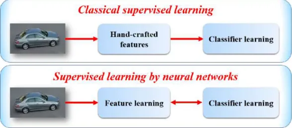
2.3.1.2 Differentiation of neural networks

Neural networks present a part of the automatic learning tools and are especially used for supervised learning. They are part of a logic that is slightly-different from "classical" learning approaches. Indeed, we previously saw that the learning process includes a step of extracting visual characteristics from the image. This step was mostly based on image-processing-oriented algorithms. Although very relevant to certain vision tasks, these characteristics may prove ineffective depending on the nature of the problem to be solved. These lead us to ask several questions. What really characterizes objects ? Are they contours ? or colors ? How can we succeed in

(29)

finding a reduced representation of an image that is as relevant and discriminatory as possible ?

It is on this point that neural networks mark a technological break. Indeed, rather than extracting visual characteristics "manually", neural networks allow the directly use of an input image and learning which visual characteristics are the most relevant for a given problem. Figure 2.7 depicts this difference. In contrast to the HOG [Dalal 2005] or SIFT [Lowe 1999] characteristics, which are low-level image representations, the neural networks permit, by a succession of non-linear functions, the extraction of increasingly high-level characteristics. It is this succession of func-tions that gives the name of Deep learning to approaches based on modern neural networks. The more functions, the deeper the network and the high level of the extracted visual characteristics.

Figure 2.7: Interest of neural networks for visual feature learning in comparison with classical supervised learning approaches (translated from a presentation of Yann LeCun 2016, Paris).

2.3.2 Neural networks: Basic concept

In this section, we propose to expose basic concept of the neural networks. We first present the basic entity of neural network, the formal neuron. Then we present the Multi-Layer Perceptron (MLP).

2.3.2.1 The formal neuron:

Formal neuron (or artificial), initially introduced in [McCulloch 1943], is a mathe-matical modeling of the biological neuron. It consists of a mathemathe-matical function to be applied to a signal and return an activation value. Considering an input signal X = {x}n=1,..,N, the artificial neuron returns the activation value y. The latter

(30)

value is computed as follows, equation (2.1):

y = f (b +

N

X

n=1

wkxk) (2.1)

In this formulation, w_i are commonly called weights and b is called bias. The function f is called an activation function. In the initial formal neuron, this function is the signal function, hence returning a binary value at the output of the neuron. The weights, the bias and the activation function characterize the formal neuron. Figure2.8 illustrates how this neuron works.

Figure 2.8: The artificial neuron.

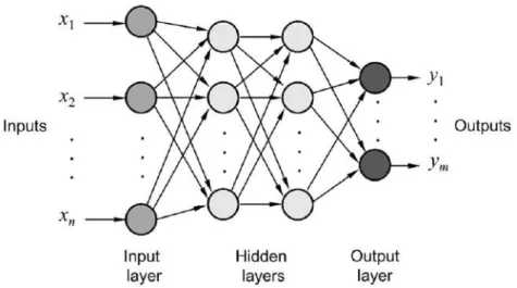
2.3.2.2 Multi-layer perceptron

The neuron has two disadvantages. It expresses only a linear relation between the inputs and its output. Moreover, its power of expression is limited since it produces only one output. The MLP was invented to overcome these limitations. First, the activation function has been modified to include nonlinearity. A popular choice of this function is the sigmoid one as it is an approximation of the derivable Heaviside function which is an essential element during learning. The second contribution of the MLP consists in connecting several neurons together as layers.

An MLP consists of three types of layers:

• An input layer that corresponds to the input data x = [x1, ..., xn].

• An output layer consisting of m neurons and producing the outputs of the network y = [y1, ..., ym], that is to say the output values associated with the

input data x.

• Hidden layers each consisting of several neurons. These layers allow the non-linear transformation of the input signal to the output one.

In the framework of the MLP, all the neurons of a layer are connected to the neurons of the previous layer. Figure2.9illustrates an MLP consisting of two hidden layers.

(31)

Figure 2.9: An example of an MLP consisting of two hidden layers. Each circle represents a formal neuron.

2.3.3 Deep convolutional neural networks

CNNs are a special type of neural networks that can be easily applied to images in order to extract and classify information spatially. The first CNN was introduced in the late 1980s by LeCun et al. [LeCun 1989] for image recognition. This network allowed the recognition of handwritten digits.

The idea is to pass an input image in a succession of convolutional filters (as shown in Figure 2.10) providing a reduced and relevant description of an image.

Figure 2.10: Examples of convolution filters: 96 filters of the first layer of AlexNet architecture [Kataoka 2015].

These characteristics are then sent to an MLP composed of hidden layers and fully connected output ones permitting classification of digits presented in the image. Convolution filters and fully connected layers are learned simultaneously. Figure 2.11 presents the architecture of a convolutional network.

Because of their convolutional structure, CNN makes it possible to take in input data of large dimension, which is a limit of the MLP.

For example, an image having three channels (RGB) of size 224 × 224 pixels rep-resents an input vector of size 150, 528 for an MLP. This involves 150, 528 weights

(32)

Figure 2.11: A convolutional network for the recognition of handwritten digits. Source [LeCun 1998]

to learn for each neuron of the hidden layer connected to the inputs, which is com-plicated to learn. The CNNs can be seen as a series assembly of modules allowing the extraction of characteristics from the pixels of an image in a hierarchical way.

2.3.3.1 Different modules of CNN

We present here the different modules used in CNNs: convolution, pooling, acti-vation functions, dropout, batch normalization and standard error functions (loss functions) used for learning.

Convolution: The core of a CNN is the convolutional layer. The resulting out-put is called feature map. A convolutional layer is made up of several convolutional filters (or kernels) to be applied to each position of an input image.

Figure 2.12 shows how the convolution works. In practice, a value (bias) as-sociated with the convolution filter is added to each position of the output of the filter. During learning, the values of the weights and biases of the neurons present the components of these filters that are learnt.

A filter of a convolutional layer is applied to all the positions of an input image, that is why we speak of shared weights.

Pooling: The pooling layer adds a spatial invariance when extracting fea-tures, reducing the size of inputs. It can be of different nature but the most used pooling types are M ax P ooling (shown in Figure2.13) and Average pooling. M ax P ooling permits returning the maximum element of a computation window. Average P ooling allows returning the average of the elements on a computation window.

Activation functions: There are different activation functions allowing the non-linearity in the different CNN layers. The most famous of these functions are (as shown in Figure 2.14): The sigmoid function, the hyperbolic tangent function and the ReLU function.

The ReLU activation function is the most used in deep CNNs because it permits easier optimization. It has the advantage of providing sparse answers and makes it possible to reduce the problems of gradient disappearance. The ReLU function, for

(33)

Figure 2.12: Convolution illustration. Given an input, a convolution filter (or con-volution kernel) is applied for each position.The depth of the kernel depends on the depth of the input to which it is applied: In this example, the input has three chan-nels, so the depth of the kernel is three. The result for a given position corresponds to the sum of the multiplication of the kernel elements by those of the input: In this example, 2 × (−4) + 5 × 2. In the context of CNNs, the output of a convolution is called a feature map. The number of feature maps depends on the number of filters applied to the input. Source [Guerry 2017]

its part, refers to a constant gradient for a large input, enabling faster learning (in particular networks with a certain depth). There are other activation functions in the same family as ReLU such as LReLU [Maas 2013], PReLU [He 2015] and eLU [Clevert 2015].

Dropout: To avoid overfitting, the dropout layer was introduced in [Srivastava 2014]. This layer is used during learning. It allows randomly deacti-vate neurons during the different learning iterations. In other words, the dropout enables the network to learn subnets containing fewer parameters, hence, less overfit-ting subjects. This way permits learning more generic parameters that do not focus on the details of the learning dataset. Once the learning is complete, all neurons are reactivated.

Batch normalization: This technique was presented by Ioffe et al. [Ioffe 2015] in order to learn the CNNs more quickly and efficiently. It starts from the following observation: During learning, the distribution of the inputs of the different network layers changes at each iteration. This induces a permanent adaptation of CNN pa-rameters to these different distributions, which increases the learning time. The idea of batch normalization is to normalize the inputs of each layer so that their distributions are of a zero mean and a unit variance. During learning, the batch normalization layers learn parameters (a scale factor and a bias) to adjust this nor-malization: These parameters enable applying a transformation on the normalized distribution.

(34)

Figure 2.13: Illustration of M ax P ooling. In this example, the pooling kernel is of size 2 × 2 and is applied every two pixels (stride = 2). The maximum of the four elements on a window of the input matrix is kept. Source [CS2]

.

Figure 2.14: The most famous activation functions. (a) sigmoid, (b) hyperbolic tangent and (c) ReLU function. Source [CS2 ]

neural networks. These functions are dependent on the task that the network must perform (classification, regression, etc.). Here we list the most used loss functions.

• The Softmax loss function, commonly used for network optimization. It allows the maximization of the probability that an entry has to belong to one class rather than another.

• The loss function by sigmoid crossed entropy, allowing a regression on proba-bilities.

• The loss L1 smooth function, introduced in [Girshick 2015a], which permits a better optimization for regression problems.

2.3.3.2 Classical neural architectures

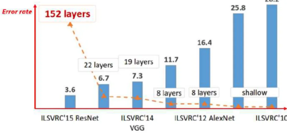
We present here the most popular architectures of the CNN used in computer vision research. It is important to note that the architectures proposed in the literature

(35)

have a strong tendency to become more and more deep with the years. In other words, it seems that the deeper the network is, the better the performances are (as shown in Figure 2.15). Nevertheless, this depth implies facing certain difficul-ties, particularly in terms of computation time and optimization during learning. This is why the community remains very active on the problem of designing CNN architectures.

Figure 2.15: Error rate of different architectures on ImageNet for object classifica-tion. Over the years, the classification error has diminished, due to the increasing depth of architectures. Source [He 2016].

Standard architectures are widely used in vision for two main reasons. The first is that they allow for an easy comparison of CNN-based methods. In other words, although some work focuses on the study of neural architectures, the majority of vision methods reuse already learned CNNs and modify them to design new architectures that respond to particular tasks. The second reason is related to the difficulty of learning deep networks because of their large number of parameters. A common practice is the use of CNNs already learnt on huge databases and then adapt them to a specific task. This is called "fine-tuning". This practice enables learning deep networks using an initialization of the weights and bias already very relevant and generic. The adaptation of these parameters is then carried out during the phase of learning the specific task that it is desired to carry out. This result in a much faster learning speed and a virtually guaranteed convergence.

AlexNet: This architecture is the one proposed in [Krizhevsky 2012], which allows the resurgence of the study of neural networks from 2012, in particular thanks to the victory at the ImageNet image classification competition. This architecture uses five layers of convolution and three layers of pooling. The size of the convolution kernels is variable (11 × 11, 5 × 5, 3 × 3) as a function of the layer in question. The activation function used between each layer is the ReLU function. After passing the image in the convolution, pooling and activation layers, a feature map is obtained. This is sent in an MLP consisting of two hidden layers and one output layer. Figure 2.16 illustrates the architecture of AlexNet.

(36)

Figure 2.16: Illustration of AlexNet architecture [Kataoka 2015].

VGG: This CNN was introduced in [Simonyan 2014]. Instead of using a single convolution per depth level such as AlexNet, this architecture utilizes convolution se-quences. In addition, VGG has convolutional filters with small size than in AlexNet (size 3 × 3). Figure 2.17presents the architecture of the VGG.

Figure 2.17: Illustration of the VGG architecture [Simonyan 2014].

ResNet: This CNN was presented in [He 2016]. It allows the learning of very deep networks (more than 150 layers). The difficulty in learning such deep networks is particularly related to the retropropagation of the gradient. The deeper the network is, the lower the gradient is for updating the weights of the lowest layers (the first layers). The idea developed in ResNet is the use of residual connections allowing better optimization of very deep networks. A residual connection makes it possible to pass the input in two convolution filters but also to pass this input directly to the following layers. This is done by summing the result of the two convolution layers and the input, as shown in Figure2.18.

(37)

Figure 2.18: Residual connection. [He 2016].

deep networks and propose a way to learn them effectively. Figure 2.19depicts the architecture of ResNet.

Figure 2.19: Illustration of ResNet architecture. Source [He 2016].

2.4 Convolutional neural networks for object detection

One of the most uses of CNNs is to localize and detect objects in images. This last problem, is a more challenging one, and requires to localize in an image sev-eral objects that can vary on size and pose. Some of the datasets challenges and competitions have contributed to the development of approaches and other CNNs architectures able to solve the object detection challenges.

As mentioned in section 2.2.1, initial approaches use well known sliding window and strategy in combination with CNNs-extracted features and a final classifier. However, Sermanet et al. provided in their approach [Sermanet 2013] that end-to-end trained CNN models can also be designed to generate an algorithm to object localization, detection and recognition. They utlized CNN special characteristics of location invariance and weights sharing to create an efficient sliding window approach. They also suggest an original approach that learns to predict object boundaries to create bounding boxes, all in the same CNN architecture.

Accordingly to section 2.2.2, the recent advancement of region proposal methods (e.g, [Uijlings 2013]) have suggested new CNNs architectures. An important one,

(38)

2.5. Transfer learning 27

was put forward by Girshick et al. [Girshick 2014b], as what is known Region-based CNNs (R-CNNs). It starts with the selective search strategy that outputs 2000 proposals. Next, it uses a pre-trained AlexNet classification model to extract a 4096 feature vector for each of the regions. Finally, it classifies each region with the SVM and with the results they fine-tune the CNN for detection.

Further works on object detection with CNNs have focused mainly on reducing the computations of R-CNNs, which has been achieved successfully by sharing the convolutions across proposals [Girshick 2015a], [Ren 2015c], [Redmon 2016a]. Dif-ferently, work done by Shaoqing et al. in [Ren 2015c], directly proposes a fully convolutional network able to produce the region proposals by adding two convolu-tional layers to the network.

Some recent research is dedicated to unifying the two-staged approach from [Ren 2015c] into one stage, avoiding to resample features. Single Shot MultiBox Detector (SSD) [Liu 2016] uses the strategy of anchors from [Ren 2015c] proposal network and applies them to several feature maps of different resolution in the convolution network. This allows the detector to consider image regions at different sizes and different resolutions for detection objects at multiple scales.

Table 2.2provides an overview of detection methods by CNN and their results on Pascal VOC 2007 [Everingham 2010].

Table 2.1: Summary of detection methods by CNN and results on Pascal VOC 2007 [Everingham 2010].

Method frame per second mAP

DSOD [Shen 2017] 17.4 77.7%

MobileNet-SSD [Howard 2017] 93 75.4%

R-CNN OHEM [Shrivastava 2016] – 78.9%

Yolo v2 [Redmon 2016b] 67 76.8%

SSD [Liu 2016] 59 74.3%

Yolo [Redmon 2016a] 45 63.4%

Faster R-CNN [Ren 2015c] 17 73.2%

Fast R-CNN [Girshick 2015a] 10 70.0%

R-CNN [Girshick 2014b] 0.1 62%

2.5 Transfer learning

Several traditional automatic learning methods operate under a common assump-tion: The learning and test data come from the same feature space and share the same sample distribution. If the distribution is different, it will be necessary to resume learning from scratch while collecting new data from the target domain and handling the tasks differently. However, in many real-world applications, the collection of new data is costly and sometimes difficult [Pan 2010b].

(39)

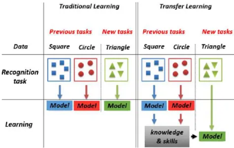
Transfer learning aims to solve this situation by developing methods to transfer knowledge and skills learned in one or more source tasks in order to use it to im-prove a target task with the consideration of similarity links between these tasks. Figure 2.20 shows the difference between traditional learning and transfer learn-ing. The traditional learning starts the learning process from scratch of new task independently from other tasks. Whereas, the transfer learning techniques use the knowledge acquired in previous tasks when learning a new one.

Figure 2.20: Differences between traditional learning and transfer learning [Pan 2010a]

The transfer process begins with a need to learn a target task in a target domain while knowing that a set of source tasks in a source domain is available and that there is a set of relationships created at the basis of similarity between the source and target problems. Defining the target task, available source tasks that can be beneficial to improve the learning of the target task and the existing similarities between the source tasks and the target ones are the answer to the question: "Where is knowledge transfer ?".

Once the source problems, the target problem and the similarity links are spec-ified, the next step is to decide what to transfer ? How to transfer ? And when to transfer ?. The question "What to transfer ?" determines the type of knowledge to be transferred from the source domain to the target one. The question "How to transfer ?" determines the nature of the transfer, that is to say whether the trans-ferred knowledge will be used as it is or whether it must undergo transformations to adapt to the new conditions. It also defines how to use this knowledge during the learning phase of the new task. The question "When to transfer ?" must assess the situation in which the transfer may be advantageous. This question seeks to avoid any case of negative transfer by determining the amount of transfer from the defined sources. If the source tasks are not similar to the target and/or if there is

(40)

2.5. Transfer learning 29

a sufficient amount of data for target task learning, transfer can result in negative effects instead of improving the learning process [Aytar 2014].

2.5.1 Motivation of transfer learning

The aim of transfer learning is to improve the learning of a target task by bringing back the knowledge learned about other source tasks. The transfer learning has several advantages, such as avoiding the manual effort required to annotate a large amount of data. Figure 2.21 describes three levels of performance improvement of transfer learning (higher start, upper slope, higher asymptote) by comparison with the learning method of the target task without transfer.

Figure 2.21: Transfer learning advantages [Tommasi 2013,Aytar 2014]

2.5.2 Different types of transfer learning

According to [Pan 2010a], there are three types of transfer learning based on the different relationships between the tasks and the source and target domains. Figure 2.22summarizes the different types of transfer learning.

Figure 2.22: Different types of transfer learning. Translated from a presentation of Houda MAAMATOU [Maâmatou 2016a], Italy.

Inductive transfer learning: For this type of transfer, the source and target domains can be similar or not, but the tasks are different. Some annotated target

(41)

data are needed to produce a predicative model to be used in the target domain. There are two cases:

• Inductive transfer learning with annotated source data: There interest in transferring source knowledge is to achieve a high performance in the real-ization of the target task. This type of transfer is similar to the multi-task learning configuration, with the difference that multi-task learning learns both source and target tasks simultaneously [Pan 2010a].

• An inductive transfer learning without annotated source data: This is a config-uration similar to a self-learning case as presented by Raina et al. [Raina 2007]. This is a situation where the source and target label spaces are different and the knowledge of the source domain cannot be used directly [Pan 2010a]. Transductive transfer learning: The transductive type deals with a target domain without any labelled data and assumes that the distribution of the source domain is different from the target one, though they are actually related. Two cases arise depending on the situation of the source and target domains:

• The characteristic spaces between the source and target domains are different.

• The characteristic spaces between the source and target domains are similar, but the distributions of marginal probabilities are different. In this type of transfer, we find the adaptation of a face detector to specific photos for a good manipulation of the new domain conditions [Jain 2011], we find also the transfer for text classification [Daume III 2006] and the adaptation of a generic pedestrian detector to a new scene [Wang 2011] [Maâmatou 2016d].

Unsupervised transfer learning: As for inductive transfer learning, the source and target tasks are different and the domains may be similar or not. How-ever in this type of learning there is no data labelled either in the source domain or in the target one. The target task is often an unsupervised problem such as grouping, dimension reduction, or density estimation. As an example, we mention the work of Dai et al., [Dai 2008] which presents an unsupervised transfer approach for grouping a set of data in the target domain by exploiting a large quantity of unlabeled data available in the source domain but learning a common feature space across domains.

In our work, we are interested on the transductive transfer learning type. The latter allows avoiding data labelling in each scene and offers improving object de-tection in different sequences. These were the reasons that motivate us to suggest an original formalization of transductive transfer learning in order to specialize a generic deep detector to a target domain.

The details of the transductive transfer learning methods are described in the following sections.

(42)

2.6. Categorization of transductive transfer learning methods 31

2.6 Categorization of transductive transfer learning

methods

The existing transfer learning methods are categorized according to the knowledge transferred. These transfer learning categories will be described in the next subsec-tions.

2.6.1 Transfer of example

These methods focus on the transfer of source examples that can be reused by solving the target task. Nevertheless, the source data may not be usable in their raw forms and may not all be useful, but some examples can reinforce the target learning process following a ponderation function. Despite the use of source and target examples, the transfer of examples learns only the target task. There are several methods of transfer of examples that are described for artificial intelligence and computer vision applications.

Haung et al. [Huang 2006] proposed a Kernel-Mean Matching (KMM) algorithm for the direct learning of the ratio of the source distribution to the target distribution by matching the two averages of the source and target data by producing a Hilbert kernel space. The main benefit of using the KMM is the ability to avoid the density estimation for both domains which can be difficult if the dataset is reduced.

Dai et al. [Dai 2007] had a "TrAdaBoost" extension of the basic doping algo-rithm "Adaboost". It reduces the weight of instances that are poorly predicted in order to reduce as much as possible their undesirable effect on the learning process. TrAdaBoost allows the construction of a good quality classification model while us-ing data of different distributions and quantities: a reduced amount of labeled data from a target distribution that is generally insufficient for learning a good classifier and a large amount of data from another source distribution. At each iteration, if an instance is badly predicted then the algorithm reduces its learning weight to attenuate its effect at subsequent iterations. In this way, examples that are not similar to the new data affect the learning process from one iteration to another. However, older instances that are consistent with recent data help the algorithm better train the classifier.

Jiang and Zhai [Jiang 2007] proposed a heuristic method to minimize the dif-ference in the conditional probabilities of the source and target domains by remov-ing samples that would disrupt target learnremov-ing. Duan [Jiang 2007] put forward a "Domain Transfer SVM (DTSVM)" approach for a video classification task. The DTSVM minimized the SVM structural risk function and the maximum average divergence. This was the criterion that identified the difference between the distri-bution of source and target samples by learning an optimized kernel function.

Sugiyama et al. [Sugiyama 2008] put forward an algorithm known as the Kullback-Leibler Importance Estimation Procedure (KLIEP) to directly estimate the ratio of source density according to target density based on the minimization of the Kullback-Leibler divergence. The KLIEP can be integrated into cross-validation