Simulation of the Noise Induced by Corona Discharges on a Ground VHF Antenna

HAL Id: hal-01609739

https://hal-enac.archives-ouvertes.fr/hal-01609739

HAL is a multi-disciplinary open access archive for the deposit and dissemination of sci-entific research documents, whether they are pub-lished or not. The documents may come from teaching and research institutions in France or abroad, or from public or private research centers.

L’archive ouverte pluridisciplinaire HAL, est destinée au dépôt et à la diffusion de documents scientifiques de niveau recherche, publiés ou non, émanant des établissements d’enseignement et de recherche français ou étrangers, des laboratoires publics ou privés.

on a Ground VHF Antenna

Mingtian Wang, Alexandre Chabory, Jean-Pierre Boeuf

To cite this version:

Mingtian Wang, Alexandre Chabory, Jean-Pierre Boeuf. Simulation of the Noise Induced by Corona Discharges on a Ground VHF Antenna. Progress In Electromagnetics Research Symposium, Mar 2013, Taipei, Taiwan. �hal-01609739�

Simulation of the Noise Induced by Corona Discharges on a Ground

VHF Antenna

Mingtian Wang1_{, Alexandre Chabory}1_{, and Jean-Pierre Boeuf}2 1_{ENAC, TELECOM-EMA, 7 Avenue Edouard Belin, Toulouse F-31055, France}

2_{LAPLACE, Paul Sabatier University, Toulouse, France}

Abstract— A jamming phenomenon has been observed on a ground station working in the VHF aeronautical frequency-band (118–134 MHz). We attest corona discharges are possibly the source of noise by means of on-site measurements. In order to predict the noise level, we propose a model which consists in two parts: an electrostatic simulation to localize the corona discharges, and a simulation in the frequency domain to evaluate the noise at the antenna ports. The agreement between simulation and measurement is good.

1. INTRODUCTION

A jamming phenomenon has been experienced by the french civil aviation authority (DGAC) on a ground station working in the VHF aeronautical frequency-band (118–134 MHz). This has yielded troubles in air-ground communications. This phenomenon appears in the presence of a strong natural electrostatic field, and is probably due to corona discharges located near the ground antennas. The corona discharges can be sources of VHF and HF noise. This is notably known for antennas onboard aircrafts and for antennas placed near high-voltage transmission lines [1–3].

In this paper, we attest that the noise source is probably corona discharges by means of on-site measurements. Besides, a model is proposed to predict the level of noise introduced by corona dis-charges at the output of VHF ground antennas. It consists of two parts: an electrostatic simulation to localize where corona discharges occur, and a simulation in the frequency domain to evaluate the noise at the antenna ports.

In the first section, the jamming phenomenon and the measurement to identify its origin are presented. In the second and the third sections, both parts of the model are presented. In the last section the simulation results are compared with measurements.

2. PRESENTATION OF THE JAMMING PHENOMENON AND ITS ORIGIN

The ground station working in the VHF aeronautical frequency band is constituted by a 40-meters high metallic pylon presented in Figure 1. There are two types of VHF antennas on the pylon. On top are placed ground-plane antennas. On lower positions are placed two circular arrays of dipoles with reflectors. They are located 3 m and 10 m below the top.

In order to find the origin of the noise, on-site measurements of the ambient electrostatic field have been performed by means of an electric field mill which is placed below the pylon, on the roof

(a) (b)

(c)

(d)

Figure 1: Configuration: (a) ground station; (b) pylon and antennas; (c) ground-plane antenna and (d) cir-cular array of dipoles with reflectors.

of the building represented in Figure 1(a). During several days, the antenna output signal and the electrostatic field have been recorded and compared.

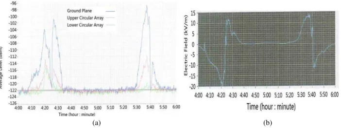
A representative case of measured data is displayed in Figure 2 for the antenna output power and electrostatic field.

The results show that there exists a clear correlation between both measurements. The level of noise always increases simultaneously with the electrostatic field, and the two phenomena last the same time. It should be noticed that this correlation between both measurements has been observed many times in the measured data. Thus, electrostatic discharges, and more particularly corona discharges may be the source of noise.

3. ELECTROSTATIC SIMULATION

Now that we have found a possible origin for the jamming phenomenon, the next work is to search for a method to predict the noise. In order to do that, an electrostatic simulation is performed to locate the place where the electrostatic field is the strongest. That is also the place where corona discharges most probably occur. For the electrostatic simulation, we suppose that the charge density is negligible in the atmosphere before the discharges occur, so the electrostatic simulation can be expressed via the Laplace’s equation ∇2_{V = 0. The models of the pylon and the antenna} are presented in Figure 3.

The model of the pylon is based on the pylon of the ground station which has been presented in the previous section. The pylon has a 4 m high lightning conductor on top. The ground plane antennas and the dipoles of the circular arrays are represented by metallic cylinders.

We assume the computation volume is a box with the pylon at its centre. For the boundary conditions, two electrodes are defined as shown in Figure 3: a sky electrode associated with the charged cloud located above the pylon, and a ground electrode constituted by the pylon and the ground. The potential difference between both electrodes is fixed so that the ambient electrostatic field corresponds to the real case. Then we assume that the computation domain is large enough, and the lateral boundaries are placed far enough from the pylon, so that the horizontal component of the electrostatic field is zero on the surface of the lateral boundaries, which corresponds to Neumann boundary conditions for the potential. The numerical simulation is realised via Comsol and is thus based on the finite element method.

From [2] and the experimental result in Figure 2(b), the ambient electrostatic field can reach a level of 20 kV/m, and the distance between the sky electrode and the ground is 60 m in our case, therefore the potential difference between electrodes is set to 20 kV/m × 60 m = 1.2 × 106_{V. The} result of the electrostatic simulation is presented in Figure 4.

The result shows that the place with the strongest electrostatic field is the tip of the lightning conductor. Compared with the other places, the electrostatic field around the upper tips of the ground plane antennas is also relatively strong, but weaker than the field of the lightning conductor. In order to locate the places where the corona occurs, the critical electric field of corona ignition shoud be evaluated. The Peek’s formula is used to evaluate the corona inception electric field E_c

(a) (b)

Figure 2: Comparison between noise (dBm) received by (a) the VHF antennas and electrostatic field (kV/m) measured by the field mill.

(a) (b) (c) Figure 3: Model for the electrostatic simulation: (a) complete pylon; (b) antennas; (c) computation volume and electrodes.

Figure 4: Electrostatic field near the top of the pylon (V/m). as [8] Ec= E0δ µ 1 +0.301√ δr ¶ (1) where E₀ = 29.8 kV/cm, r is the radius of the conductor in cm, δ is the ratio of air density to the normal density corresponding to p = 760 Torr and T = 25◦_{C. In our case, the radius of}

the lightning conductor is 5 cm, and we assume that δ = 1, so the critical electric field E_c = 33.8 kV/cm = 3.38 × 106_V/m.

The simulation result in Figure 4 shows that the surface of the tip of the lightning conductor is the only place where the electric field is stronger than the critical electric field. Thus the top of the lightning conductor is the place where the corona discharges most probably occurs.

4. SIMULATION IN THE VHF FREQUENCY DOMAIN

In the previous section, the place where corona discharges occur has been found. We are going to perform the simulation in the VHF frequency domain to verify the noise level generated by corona discharges.

The simulations in the VHF frequency domain are performed via Feko. We model the pylon as a wire structure because the section of the tubes is small compared with the wavelength (2 m). Both types of VHF ground antennas are modeled so as to obtain realistic matchings and radiation patterns. The voltage standing wave ratio (VSWR) and the gain patterns are presented in Fig-ure 5. For both types of antennas, the VSWR is below 1.5 in all the aeronautical VHF frequency bandwidth. Besides, in the horizontal plane, the radiation patterns are quasi omnidirectional. In the vertical plane, the half-power beamwidths are about 70◦ and 90◦ for the ground plane and circulare array, respectively.

The corona discharges in the VHF band are represented by short electric dipoles [4] placed where the corona discharge would occur, i.e., on the top of the lightning conductor.

In [6], the current of the corona discharge can be represented by the following equation

I(t) = KIp

³

e−αt− e−βt

´

, (2)

where I(t) is the current of the corona discharge, Ip is the peak value of the corona discharge

current, α and β are constants, and K is a coefficient depending on α and β. In [6], the following values are found by means of measurements: α = 0.01 ns−1_{, β = 0.0345 ns}−1_{, K = 2.34. In [7],}

a representative value of the peak corona discharge current is estimated as Ip = 10 mA. From a

Fourier transform of (2), we find that the corona discharge current in the VHF band is about 1µA. Based on the experimental results of [4, 5], we assume that the corona current is concentrated in an area about 5 cm around the corona point. Thus the dipolar moment is chosen to be 5 × 10−8_{A · m.}

To determine the noise introduced by the corona discharges, we simulate the power at the antenna ports when they are excited by the short dipoles.

(a) (b) (c)

Figure 5: Matching and gain patterns of models of both antennas: (a) voltage standing wave ratio; (b) gain pattern (dBi) in the horizontal; (c) in the vertical plane.

Figure 6: Power received at the ports of the antennas in the VHF frequency domain (dBm).

5. COMPARISON WITH THE EXPERIMENTAL RESULTS

The simulation result in the VHF frequency domain is presented in Figure 6. In the aeronautical VHF band, the noise received by the ground plane antenna located on the top of the pylon can reach −91 dBm. The antenna output noise measured during the experiments has been presented in Figure 2. In this figure, the maximal noise received by the ground plane VHF antenna in the VHF band is about −96 dBm. Thus there is a good agreement between the simulation result and the experimental one.

6. CONCLUSION

The corona discharges have been found as a possible origin of the jamming phenomenon observed on a ground station working in the VHF aeronautical frequency-band. A model has been proposed to predict the noise level induced by corona discharges at the ports of the VHF antennas. The place where the corona discharges occurr has been localized via an electrostatic simulation. The simulation results of the received noise level at the ports of the antennas are in good agreement with the measurements.

ACKNOWLEDGMENT

The authors acknowledge the financial support of PRES University of Toulouse, R´egion Midi-Pyr´en´ees and DGAC (french civil aviation authority).

REFERENCES

1. Fu, H., Y. Xie, and J. Zhang, “Analysis of corona discharge interference on antennas on composite airplanes,” IEEE Transactions on Electromagnetic Compatibility, Vol. 50, No. 4, 822–827, Nov. 2008.

2. Page, H. and D. J. Whythe, “Corona and precipitation interference in v.h.f. television recep-tion,” Proceedings of the Institution of Electrical Engineers, Vol. 114, No. 5, 566–576, May 1967. 3. Olsen, R. G. and B. O. Stimson, “Predicting VHF/UHF electromagnetic noise from corona on power-line conductors,” IEEE Transactions on Electromagnetic Compatibility, Vol. 30, No. 1, 13–22, Feb. 1988.

4. Wilson, P. F. and M. T. Ma, “Fields radiated by electrostatic discharges,” IEEE Transactions

on Electromagnetic Compatibility, Vol. 33, No. 1, 10–18, Feb. 1991.

5. Fujiwara, O., “An analytical approach to model indirect effect caused by electrostatic dis-charge,” IEICE Transactions on Communications, Vol. E79-B, No. 4, 483–489, Apr. 1996. 6. Rakoshdas, B., “Pulses and radio-influence voltage of direct-voltage corona,” IEEE

Transac-tions on Power Apparatus and Systems, Vol. 83, No. 5, 483–491, May 1964.

7. Janischewskyj, W. and A. Arainy, “Corona characteristics of simulated rain,” IEEE

Transac-tions on Power Apparatus and Systems, Vol. 100, No. 2, 539–551, Feb. 1981.

8. Xu, M., Z. Tan, and K. Li, “Modified peek formula for calculating positive DC Corona incep-tion electric field under variable humidity,” IEEE Transacincep-tions on Dielectrics and Electrical

Insulation, Vol. 19, No. 4, 1377–1382, Aug. 2012.

9. McLean, K. J. and I. A. Ansari, “Calculation of the rod-plane voltage/current characteristics using the saturated current density equation and Warburg’s law,” IEE Proceedings A Physical

Science, Measurement and Instrumentation, Management and Education — Reviews, Vol. 134,