HAL Id: hal-00513657
https://hal.archives-ouvertes.fr/hal-00513657
Submitted on 1 Sep 2010
HAL is a multi-disciplinary open access
archive for the deposit and dissemination of
sci-entific research documents, whether they are
pub-lished or not. The documents may come from
teaching and research institutions in France or
L’archive ouverte pluridisciplinaire HAL, est
destinée au dépôt et à la diffusion de documents
scientifiques de niveau recherche, publiés ou non,
émanant des établissements d’enseignement et de
recherche français ou étrangers, des laboratoires
solution
Laurent Proville, David Rodney, Yves Jm Brechet, Georges Martin
To cite this version:
Laurent Proville, David Rodney, Yves Jm Brechet, Georges Martin. Atomic-scale study of dislocation
glide in a model solid solution. Philosophical Magazine, Taylor & Francis, 2006, 86 (25-26),
pp.3893-3920. �10.1080/14786430600567721�. �hal-00513657�
For Peer Review Only
Atomic-scale study of dislocation glide in a model solid
solution
Journal: Philosophical Magazine & Philosophical Magazine Letters Manuscript ID: TPHM-05-Dec-0539.R2
Journal Selection: Philosophical Magazine Date Submitted by the
Author: 05-Jan-2006
Complete List of Authors: Proville, Laurent; CEA, SRMP Rodney, David; ENSPG, GPM2 Brechet, Yves; INPG, ltpcm Martin, Georges; CEA, siége
Keywords: strengthening mechanisms, atomistic simulation, dislocation interactions, solid solutions
Keywords (user supplied):
Note: The following files were submitted by the author for peer review, but cannot be converted to PDF. You must view these files (e.g. movies) online.
For Peer Review Only
Atomic-scale study of dislocation glide in a model solid solution
L. PROVILLE1∗ and D. RODNEY2, Y. BRECHET3 and G. MARTIN11 Service de Recherches de M´etallurgie Physique,
CEA-Saclay/DEN/DMN 91191-Gif-sur-Yvette Cedex, France
2
GPM2/ENSPG, Domaine Universitaire BP 46, 38402 St Martin d’H´eres Cedex, France
3 LTPCM/ENSEEG, Domaine Universitaire BP 75, 38402 St Martin d’H´eres Cedex, France
(Dated: January 5, 2006)
Based on atomic scale simulation techniques, we study the dislocation pinning mechanism in a dilute Ni(Al) model solid solution. For a solute concentration between 1 and 10 at. %, we found that the pinning of the dislocation on obstacles made of Al pairs is an interaction that operates significantly. The statistics of the dislocation motion is then modified accordingly to the nature of the obstacles and follows a modified Mott-Nabarro statistics. Finally, a method to address thermal activation is proposed and exemplified on a periodic row of solute pairs.
Keywords: strengthening mechanisms, dislocation interactions, solid solutions, atomistic simulation
I. INTRODUCTION
Computer modelling has addressed all aspects of physical metallurgy Ref.[1, 2]. While dislocations are extended defects for which mesoscale modelling seems to be the most promising tool Ref.[3], atomic-scale modelling proved to be very fruitful for some specific issues, where the elastic theory reaches its limit (e.g. when core interactions are important)[4]. Most studies are concerned with pure metals[5, 6] while a number of classical issues in physical metal-lurgy concerns alloys [7–10]. Recently, we addressed the question of dislocation glide in concentrated solid solutions, with Ni(Al) as a prototype of such problems[11] ( CAl≈ 5 at. %). One conclusion was that the hardening mechanism
cannot reduce to the classical solute dislocation interaction but could rather be attributed to solute-solute pairs, in course of dislocation crossing. Although solid solutions have been studied experimentally for many decades[12], they are still a matter of debate, in particular because it is difficult to discriminate between theories due to the limited range of solubilities for alloying elements which have a strong interaction with the dislocations[13]. The classical scheme for describing solid solution hardening is inherited from that of dilute solution- and precipitate- hardening. In Mott-Nabarro model[7–9, 14], the increase in yield stress originates from the long-range elastic interaction between the edge part of the dislocations and the solutes. It leads to a hardening which varies as a power law of the number of solutes per unit area of the glide plane, C. A first estimation was made in the late fifties[7] that showed a linear behavior, which was later corrected[8, 14, 15] to account for dislocation wavyness, leading to C2/3. An alternative
approach, proposed by Friedel[10, 16], considers the short-range interaction between the dislocation and the pinning centers located in its glide plane. The yield stress then varies as C1/2. It is noteworthy that a transition in C has
been predicted between both aforementioned statistics[15, 17]: in diluted solid solutions Friedel statistics should apply while in concentrated solid solutions, Mott-Nabarro statistics should become more relevant[18] because in the latter case the dislocations are quasi-straight between the closely spaced obstacles. Here we note that the nature of the obstacles does not change with concentration, i.e. the solutes are assumed to remain isolated in the glide plane. In addition, since the dislocation-solute interaction was thought to be the dominant hardening mechanism, the classi-cal theories model the dislocation glide in solid solution as occurring in the potential of interaction with a ”frozen” population of solutes (i.e. solute atoms the position of which is independent of the dislocation location). In fact, in the case of a concentrated Ni(Al) solid solution (C = CAl≈ 5 at. %), we showed that a source of hardening was due
to solute-solute short range repulsion, or more specifically, was due to pairs of solute atoms brought into positions of strong mutual repulsion in the course of dislocation glide. According to that finding, the nature of the obstacles thus changes with concentration since the concentration of these pinning pairs varies as C2
Al. Since this C 2
Alis much smaller
than CAl, Friedel statistics should be relevant for the Al pairs and their contribution to hardening should be linear in
CAl(see Ref.19). From a general point of view, it is noteworthy that, if hardening is due to pairs of Al atoms that are
brought closer by dislocation sweeping, edge and screw dislocations should play similar roles by way of contrast with the earlier models where hardening originates from the hydrostatic interaction between the solute atoms and only the edge part of the dislocations. Note also that, due to the limited solubility, experimental data on solid solution hardening can equally well be fitted with C1/2 as well as C2/3 or even C [20]. In spite of these difficulties, some
∗Electronic address: laurent.proville@cea.fr
1 2 3 4 5 6 7 8 9 10 11 12 13 14 15 16 17 18 19 20 21 22 23 24 25 26 27 28 29 30 31 32 33 34 35 36 37 38 39 40 41 42 43 44 45 46 47 48 49 50 51 52 53 54 55 56 57 58 59 60
For Peer Review Only
2
experimental studies tentatively examined the role of small solute clusters in solid solution hardening and worked out exponents that differ from those shown in the standard statistics, for instance an exponent of 0.57 was found by Wille et al. Ref.[13] in Cu(Mn) and Cu(Ge) solid solutions. This contradicts the previous theoretical power laws and thus the debate still remains open.
MD simulations provide opportunities to work out interesting new elements about hardening of solid solutions. Indeed the simulations allow to investigate ideal cases such as a true random solid solution and permit to test the theories in a more reliable way. This primarily motivates our present investigations. From our previous attempt[11] to simulate dislocation glide in solid solutions with concentrations between 1 and 8 at. %, at finite temperature T = 300 K, we identified a linear statistics, i.e. a resolved shear stress τc proportional to CAl, which came as a confirmation of
the argument about the validity of Friedel statistics for Al pairs. In the present paper, we work out the details of the pinning effect of Al solutes, i.e. single solutes and pairs in different geometries. In order to do so, a well controlled geometry of regularly spaced obstacles is generated and its pinning effect on a moving dislocation is investigated. This allows us to clarify the different contributions to hardening(Sec. III). Then our study is extended to a larger range of concentrations, ranging from dilute to concentrated. The strategy is there to evaluate the density of a given type of obstacle and to weight it by its pinning strength in order to estimate an overall pinning force (Sec. IV). The effect of a finite temperature is studied (Sec. V) for a regular array of obstacles. Our notations are summarized in App.A.
II. SIMULATION METHOD AND SIMULATION CELL
To model the interatomic potential, we employ an Embedded Atom Method (EAM) which provides a good compromise between the realism of dislocation simulation and the computational load necessary to handle a system large enough to keep at least part of the complexity of the real alloy. For pure nickel we chose the potential developed by Angelo et al. which has proved to be well adapted to the atomic scale simulation of dislocations.[21, 22] In particular, the dissociation width of the edge dislocation is quantitatively well reproduced by this potential. In our simulations, the dissociation width equals 3.3 nm, which agrees with the observations of Carter and Holmes[23] who estimate this width, between 1.8 and 3.6 nm. For pure aluminum we chose the potential proposed by Voter and Chen,[24] which has the drawback of yielding a low stacking fault energy (compared e.g. to the potential of Ercolessi et al.[25]), but has the advantage of being written in the very same functional form as that for Ni. The interaction potential between Ni and Al has been developed to account for the physics of alloys NiAl and Ni3Al. The form and the optimization of this potential are described elsewhere[11]. The
reader interested in more detailed information about the simulation technique and physical properties of the NiAl solid solution model we use, is referred to Ref.[11].
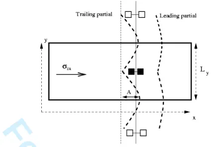
The simulation cell is schematically represented in Fig.1. It is oriented so that the horizontal Z planes are (1¯11) planes while the X direction is a [110] Burgers vector direction. An edge dislocation is introduced between the two (1¯11) central mid-planes of the cell with a line oriented along the [¯112] Y direction. The simulation box size along the different directions, i = X, Y, Z is denoted by Liand the Ni lattice parameter by a0. The dislocation core is dissociated
in two partials and the atoms that take part into the partials are recognized by their default configurations in first neighbor positions. Periodic boundary conditions are applied both parallel and perpendicular to the dislocation line. In Fig. 1, we show an Al pair (filled squares), with its first periodic images (open squares). Because of the periodic boundary conditions imposed along the dislocation line, i.e. in the [¯112] direction, a chain of obstacles is formed with a spacing L which equals Ly, the size of the simulation box in the Y direction (see Fig. 1).
For the Molecular Statics (MS) simulations (at 0 K), we use a Gradient algorithm, which is a minimization of the total potential energy, achieved through a gradient procedure under a fixed applied shear stress. The applied stress τzx is produced by adding extra forces to the atoms in the upper and lower Z surfaces. This external applied stress
is incremented by 0.75 MPa and for each increment the gradient procedure is performed till either it converges to a required precision or the dislocation starts to glide in the cell, in which case we consider that the yield stress is reached. In Fig. 2, the average position of a dislocation has been plotted versus the increasing applied stress. The obstacles were positioned at x = 6nm in the simulation cell. Apart from the initial stage where the Peierls stress has to be overcome to force the dislocation to glide towards the obstacle, the dislocation was found to stop at two different positions (labels A and B in Fig. 2) because of its dissociation in two partials that interact differently with the obstacle. When the external stress is sufficient to unpin the trailing partial (label C in Fig. 2), the dislocation glides freely in the simulation box.
For the Molecular Dynamics (MD) simulations (at 300 K), we integrate the dynamics under a fixed τzx. It is worth
noticing that in MD simulations, the time scale is typically one nanosecond which is far from the time required to model diffusion processes in solid solutions. As a consequence, we consider ideal, purely random, solid solutions and even though this solid solution is supersaturated, precipitation cannot take place.
1 2 3 4 5 6 7 8 9 10 11 12 13 14 15 16 17 18 19 20 21 22 23 24 25 26 27 28 29 30 31 32 33 34 35 36 37 38 39 40 41 42 43 44 45 46 47 48 49 50 51 52 53 54 55 56 57 58 59 60
For Peer Review Only
FIG. 1: Schematic view of the simulation cell containing an edge dislocation and an Al pair (filled squares) along with its first periodic images (open squares).
FIG. 2: A plot of the average position of the dislocation core versus the external shear stress during Molecular Statics simulations at 0 K, for different types of obstacle (see Tab.I). The labels (A,B and C) are described in the text.
III. CASE OF PERIODIC CHAIN OF OBSTACLES: STRENGTHENING EFFECT OF DIFFERENT
PINNING CONFIGURATIONS A. Geometry of significant obstacles
Beside the classical situation of the interaction between an isolated Al atom (see Fig. 3) and a dislocation, several other configurations involving pairs of Al atoms have been tested (see Fig. 4). Regular chains of obstacles of given types were generated, with a distance L between obstacles. The shear stress necessary to glide through the array of obstacles is τc = αµb/L, where α, the interaction coefficient, characterizes the strength of the obstacle, b is the
Burgers vector and µ is the shear modulus of pure Ni. The 1/L term gives the number of obstacles per unit length of dislocation and αµb2is the maximum force exerted by each obstacle. Among the different configurations, we selected
those with highest yield stress. The dislocation may interact with Al atoms in three ways. Either it interacts with isolated Al atoms (Fig. 3) or it interacts with preexisting Al-Al pairs (Fig. 4(a) and Fig. 4(b)), or it generates such pairs by its passage Fig. 4(c-g). The investigated pinning configurations are shown in Figs.3 and 4, which represents a portion of the two central (1¯11) planes contiguous to the dislocation glide plane. Atoms in the lower (1¯11) plane are
1 2 3 4 5 6 7 8 9 10 11 12 13 14 15 16 17 18 19 20 21 22 23 24 25 26 27 28 29 30 31 32 33 34 35 36 37 38 39 40 41 42 43 44 45 46 47 48 49 50 51 52 53 54 55 56 57 58 59 60
For Peer Review Only
4
FIG. 3: Portion of the 2 nearest (1¯11) planes that bound the dislocation glide plane showing the configurations of isolated Al atoms (type I obstacles in Tab.I) that have the strongest pinning effect. The square symbol is the Al atom whereas the circles are Ni atoms. Open symbols represent atoms situated above the glide plane, the full symbols the ones below the glide plane. The arrows indicate the motion of the Al atom in the course of the shearing process.
(a)
(b)
shown as full circles, whereas those in the upper plane are represented by empty circles. The Al atoms are squares with larger sizes, in agreement with the size ratio between Al and Ni atoms (14 %). Plotting the normalized yield stress τc/µ as a function of the normalized obstacle density b/L as done in Fig. 5 gives a direct measure of α.
For isolated Al atoms (hereafter called type I ), the strongest configuration is such that the Al atom occupies a site in the (1¯11) plane just above the glide plane (see Fig. 3 (a)), so as to visit the compression zone of the core in the course of dislocation crossing. The interactions between an isolated Al and the two Shockley partials do not have same magnitude. The controlling reaction is the unpinning of the trailing partial. For a solute atom in the plane below the glide plane(see Fig. 3 (b)), the pinning coefficient of the trailing partial is weaker(see Fig. 5 (a)) than when the Al atom is in the plane above, and the pinning strength on the leading partial is negligible since it is of the same order as the Peierls stress of Ni. The strength for single Al atoms in (1¯11) planes that do not bound the dislocation glide plane has been found to be also of the order of the Peierls Ni stress.
The pair configurations shown in Fig. 4(a) and Fig. 4(b) are first-neighbor Al atoms(called type II ) placed in the plane above the glide plane. As for isolated Al, the dominant interaction is the one between the trailing partial and the Al pair with a strength α which is approximately twice the one for single Al. The strength on the leading partial depends on the direction of the dimer bond (e.g. [¯112] shown in Fig. 4(a), [011] or [10¯1] shown in Fig. 4(b)). The same pair configurations in the plane below the glide plane have strength of same order as obstacles of type I (see the dot-dashed line in Fig. 5(b)).
In configurations shown in Fig. 4(c) and Fig. 4(f), before the passage of the dislocation, the Al atoms are third and second neighbors (called type III ), respectively. One Al atom is in the lower (1¯11) plane and the other Al atom in the upper plane. As schematically depicted in Fig. 4(c) and Fig. 4(f), if the edge dislocation glides over this pair, the two solute atoms become first neighbors. This configuration is highly energetic as seen from the fact that the ordered phase in equilibrium with the solid solution of this alloy is Ni3Al, which is L12 with the Al atoms in second
neighbor positions. This energy excess is at the origin of the pinning effect on the dislocation. The glide process of the dislocation over the third neighbor Al pair comprises two stages corresponding to the passage of two Schockley partial dislocations: when the first partial glides over the Al pair, the latter is shifted by the a/6[121] Burgers vector of the leading partial and adopts an intermediate configuration; when the second partial glides over the pair, the Al atoms are brought into first neighbor positions which are the most energetic configurations. More precisely, the configuration of Fig. 4(c) (resp. Fig. 4(f)) becomes that of Fig. 4(d) (resp. Fig. 4(g)). Again, the limiting reaction is the unpinning of the second partial from the Al pair.
The nearest neighbor pairs in Fig. 4(d) and Fig. 4(g) (type IV ) proves to constitute also pinning centers with a force of same order as other pairs. The glide process on type IV obstacle in Fig. 4(d) conserves the pair of nearest neighbors, but forces the direction of the pair to flip so as to form the configuration in Fig. 4(e). The glide over this latter configuration forces the dimer to pass through a second neighbor position which is favored by the stability of the L12phase. The passage of the trailing partial breaks that bond and thus it involves a pinning force. The different
obstacles interact differently with both partials as summarized in Tab.I.[26]
B. Interaction coefficients at 0K: origin of the pinning strength
The pinning force of each type of obstacle is given by the α coefficients in Tab. I. The physical origin of the pinning force can have various contributions. The classical interpretation considers the interaction between individual solute atoms and the dislocation. This is likely to apply to type I defects. According to the elastic theory[28], the interaction
1 2 3 4 5 6 7 8 9 10 11 12 13 14 15 16 17 18 19 20 21 22 23 24 25 26 27 28 29 30 31 32 33 34 35 36 37 38 39 40 41 42 43 44 45 46 47 48 49 50 51 52 53 54 55 56 57 58 59 60
For Peer Review Only
FIG. 4: Same as Fig. 3 for the configurations of Al pairs that have the strongest pinning effect (see text for details).
(a)
(b)
(c)
(d)
(e)
(f)
(g)
potential between an edge dislocation and an impurity is:
W (~r) = βel
sinθ
r (1)
where θ is the impurity azimuthal departure from the glide plane, r the distance between the impurity and the dislocation and βel =
µbp
3π 1+ν
1−ν(vs− v) with µ, the shear modulus of Ni, bp, the edge leading partial Burger vector
(be = 0.5b), ν, Poisson’s ratio and vs and v, the atomic volumes of, respectively, the impurity (the solute) and the
matrix (the solvent). For Ni(Al) we have ν = 0.28, vs= 16.6 ˚A3, v = 11 ˚A3.
Let us consider as in the simulations, a regular chain of isolated Al atoms at the closest position from the dislocation core, i.e. z ≈ a0
√
3/2 = bp3/8. This corresponds to the inter-plane distance between planes that bound the dislocation glide plane. The X axis force sustained by the dislocation and due to one impurity is given by 2βelxz/(x2+
z2)2, the maximum of which is reached at x = z/√3. This force is rewritten as αµb2 such as to obtain a pinning
strength α = 1+ν1−ν(vs− v)/(2
√
3πb3) which yields numerically in the present case of Ni(Al): α = 0.06. This result is much larger than the one obtained from the simulations in Fig.5 at zero Kelvin, i.e. α = 0.009 for the trailing partial and α = 0.0062 for the leading partial. As it is seen from Fig. 6(a), the short range variations of the interaction
1 2 3 4 5 6 7 8 9 10 11 12 13 14 15 16 17 18 19 20 21 22 23 24 25 26 27 28 29 30 31 32 33 34 35 36 37 38 39 40 41 42 43 44 45 46 47 48 49 50 51 52 53 54 55 56 57 58 59 60
For Peer Review Only
6
FIG. 5: The yield stress τc versus the inverse of L, the distance between pinning centers along the Y axis. The computation
has been carried out by Molecular Statics at 0 K in various samples, containing different types of obstacles, detailed in the text. The stress has been normalized by the Ni shear modulus and the distance L by the Ni Burgers vector. For obstacles in the (1¯11) plane just above the glide plane, the yield stress of the trailing partial is represented as a continuous line (circle symbols), the dashed line (square symbols) corresponds to the leading partial. For obstacles in the (1¯11) plane just below the glide plane, the yield stress of the trailing partial is plotted in Fig. 5(a) and Fig. 5(b) as a dot-dashed line (triangle symbols).
(a)
(b)
(c)
(d)
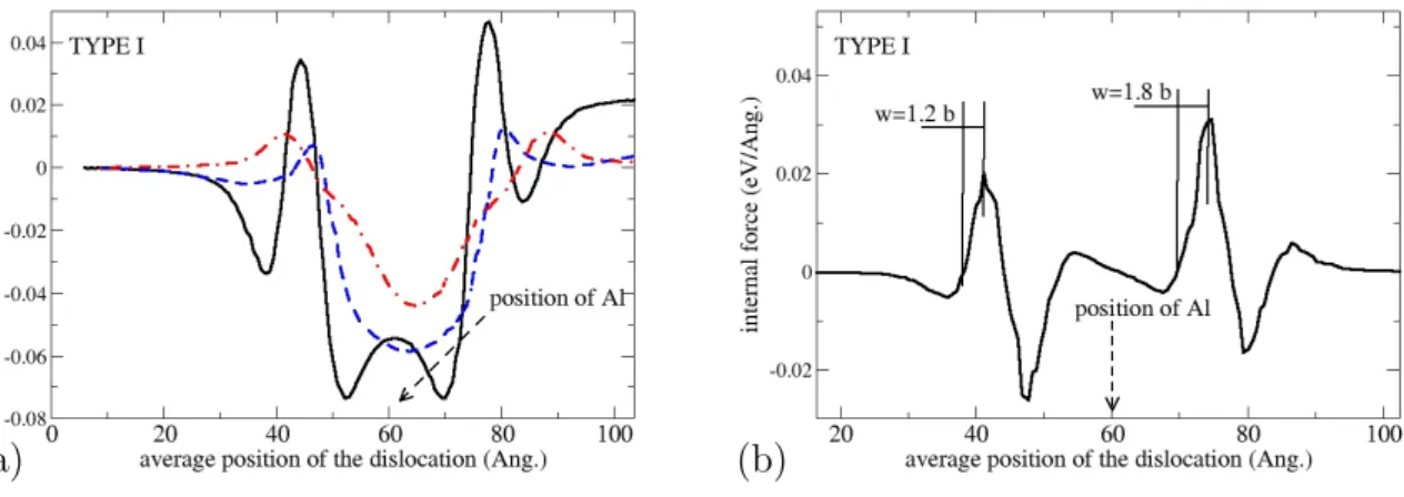
potential does not vary monotonously with distance between the dislocation and the obstacle, as assumed by an elastic interaction model as in Eq.1. On the other hand, for a single impurity in the second nearest plane above the glide plane (dot-dashed line in Fig. 6(a)), the long range repulsive interaction, expected from elastic theory is recovered. Indeed, for a distance between the average position of the dislocation core and the obstacle, larger than 20 ˚A, the internal energy increases monotonously as the distance decreases. Below this cut-off distance, which corresponds to a distance of 3 b, between the leading partial and the obstacle, the internal energy decreases to reach a minimum when the obstacle is at the center of the dislocation stacking fault ribbon. It is noteworthy that for all obstacle types, we found that the internal energy is minimum when the defect is visiting the dislocation stacking fault. This Suzuki effect[16] implies that the pinning of the trailing partial is stronger than that of the leading partial. As may be expected, this short range interaction is not properly described in the standard elastic theory as in Eq.1.
For an obstacle situated immediately above or below the glide plane, in the planes that bound the glide plane, the long range interaction is found to be attractive whereas from elastic theory one would expect that these interactions would have opposite sign, because of sinθ in Eq. 1. In fact, the position of the glide plane, situated between two atomic planes that are separated by b√3/2, is arbitrary. As this fixes the azimuthal angle θ, we have no means to determine accurately this angle for atoms in the nearest atomic planes. This concerns the long range interaction forces which strength are negligible compared to the short range forces. This can be seen from Fig. 6(b) and Fig. 7. Moreover the long range forces with different directions, i.e. either pulling or retaining the dislocation are superposed
1 2 3 4 5 6 7 8 9 10 11 12 13 14 15 16 17 18 19 20 21 22 23 24 25 26 27 28 29 30 31 32 33 34 35 36 37 38 39 40 41 42 43 44 45 46 47 48 49 50 51 52 53 54 55 56 57 58 59 60
For Peer Review Only
type Nature Schema α and w of leading α and w of trailing partial pinning partial pinning type I single Fig. 3 (a) 0.0062/ 1.2b 0.009/ 1.8b
Fig. 3 (b) 0.001/ 2b 0.004/ 3b type II 1st neighbor Fig. 4 (a) 0.018/ 2.4b 0.021/ 3.6b
non-crossing pair Fig. 4 (b) 0.01/ 2.4b 0.019/ 3.6b type III 3rd neighbor Fig. 4 (c) < 0.003/ < b 0.017/ 4b
crossing pair Fig. 4 (f) < 0.003/ < b 0.018/ 4b type IV 1st neighbor Fig. 4 (d) 0.013/ 2.5b 0.017/ 3.7b
crossing pair Fig. 4 (e) < 0.003/ < b 0.018/ 3.6b Fig. 4 (g) 0.009/ 2.4b 0.012/ 3.6b
TABLE I: Summary of different pinning configurations, the manner they interact with the dissociated edge dislocation, their normalized pinning force α and the force range w.
linearly and thus compensate provided the solute concentration is large enough to give a quasi-uniform distribution in a shell that surrounds the dislocation core[9].
In the case of type II dimers, the interactions are expected to result from the size effect of the solute atoms. Indeed, we found that the type II pinning coefficients are approximately twice that of type I obstacles, in agreement with the elastic theory where interactions add linearly. The case of type III and IV dimers is different. If we consider third neighbor pairs of solute atoms across the dislocation glide plane, then according to Eq. 1, the dislocation is attracted by the Al atom in the lower plane and repelled by the one in the upper plane. Both effects compensate at first order and thus, from the elastic theory, the interaction between the edge dislocation and the dimer is expected to be much weaker than for a single atom. This prediction of the elastic theory is not verified as shown in Tab. I. The pinning force for type III and IV is much larger than for single atoms. The physical reason is that in these configurations, the dominant pinning effect is not to the solute-dislocation elastic interactions, but rather to the solute-solute interaction that is either repulsive or attractive.
In the plane below the glide plane, we noticed that the pinning forces of dimers are comparable or smaller that of single Al atoms, depending on which partial is considered. Placing pairs in second nearest neighboring (1¯11) planes, above or below the glide plane does not lead to a yield stress larger than single Al atoms in same planes. This will allow us to neglect the role of pairs in configurations that are placed far from the plane above the glide plane. In these cases, the interaction between the dislocation and solutes could be well approached by considering only type I obstacles.
C. Range of the interactions
In the previous section we quantified the strength of the individual obstacles. In the classical theory of collective pinning[14] an other quantity of interest is the range of the interactions. To measure that range, it is sufficient to calculate the variation of the internal energy of a system under a prescribed stress containing a dislocation which adapts its position. The internal energy is obtained from the sum of all the atomic potential energy at the convergence of each step of the energy minimization procedure under increasing applied stress. This has been done in Fig. 6(a) for type I obstacle. The calculation of the first derivative of the internal energy with respect to the average position of the dislocation is plotted in Fig. 6(b). The positive part of that quantity corresponds to the internal force which is opposed to the dislocation displacement. The range of the interaction between an obstacle of a given type and the dislocation is estimated from the distance which separates the maximum of the force and the nearest position where the force falls to zero. The calculation has also been carried out for different pairs, which is exemplified in Fig. 7. The results for all types are reported in Tab.I. As expected from simple considerations on the size of the obstacles, the range of interaction is of order of the atomic spacing for type I obstacles, and 2 to 3 atomic spacings for type II, III and IV pairs.
IV. SOLUTE HARDENING IN RANDOM SOLID SOLUTION AT 0 K
A. Density of different obstacles
From the previous results, the solid solution hardening has been shown to be mainly due to the solute obstacles contained in planes that bound the glide plane. It is interesting to count the number of significant interactions with
1 2 3 4 5 6 7 8 9 10 11 12 13 14 15 16 17 18 19 20 21 22 23 24 25 26 27 28 29 30 31 32 33 34 35 36 37 38 39 40 41 42 43 44 45 46 47 48 49 50 51 52 53 54 55 56 57 58 59 60
For Peer Review Only
8
FIG. 6: In (a), internal energy of our simulation box versus the average position of the dislocation core. The simulation box contains a single obstacle of type I situated either in the plane above the glide plane (full line), in the plane below (dashed line) or in the second nearest plane above (dot-dashed line). In (b), the derivative of the internal energy for type I obstacle in the plane just above the glide plane.
(a)
(b)
FIG. 7: Plot of the internal force versus the dislocation average position. The obstacle is either a first neighbor pair (type II) (solid line) or a third neighbor pair (type III) (dashed line).
each type of obstacle in the plane above the glide plane. We denote by ni, the number of configuration per atomic
site along the dislocation line, where the obstacle type is labelled by the subscript i. As we saw in Sec.III B that a single Al above the glide plane could pin both partials, so we obtain simply nI = 2.
In case of obstacles made uniquely of pairs, we have first to enumerate the different pinning configurations. The pair configurations of type II may have 3 different bond directions and can pin either the leading partial or the trailing one. This makes 6 different possibilities to place a type II obstacle per atomic site along the dislocation line, so that nII = 6. By contrast one can consider that the interaction of type III obstacles and the leading partial is negligible.
Depending on the relative location of Al atoms in the planes that bound the glide plane we found only 2 different possibilities for type III obstacles to pin the trailing partial, so nIII = 2 . For type IV, this depends strongly on
both the direction of the pair bond and the location of Al atoms. For the leading partial, we found two significant interactions while for the trailing partial there are 3 possibilities. The total of interactions thus rises to nIV = 5. The
total number of possibilities of interaction with Al-Al pairs is thus nII+ nIII+ nIV = 13.
1 2 3 4 5 6 7 8 9 10 11 12 13 14 15 16 17 18 19 20 21 22 23 24 25 26 27 28 29 30 31 32 33 34 35 36 37 38 39 40 41 42 43 44 45 46 47 48 49 50 51 52 53 54 55 56 57 58 59 60
For Peer Review Only
B. Dislocation flexibility
For a chain of isolated Al atoms above the glide plane, the interaction coefficient α is 0.9 10−2 (see Fig. 5). The bending of a dislocation reaches a maximum at the middle of the interval between obstacles, given roughly by αL/4. To reach a value of b, L must be larger than Lb = 4b/α = 556b (138nm). According to Fig. 5(a), the corresponding
resolved shear stress (around 2 MPa) is comparable to the intrinsic lattice friction of a few MPa. So the hardening due to a chain of isolated obstacles, with L > Lb is negligible. For L < Lb the bending can be neglected and the
length of the dislocation segment between pinning point can be considered as equal to L. Similar considerations for pairs lead to Lb = 236b and to a corresponding yield stress of 12 MPa. It is noteworthy that the maximum bending
between two obstacles increases as the distance L. The number of sites that a single Al can occupy on a single partial is Ny = Ly/(b
√
3). For both partials, the proportion of Al at fixed Ly is thus 1/(nINy) for a regular chain.
Assuming the same proportion in the solid solution would involve that CAl = 1/(nINy). In this solid solution, the
mean distance between single Al alongside the Y axis is L = Ly. Replacing Ly by Lb in Ny gives CAl = 0.3 %.
Since we choose to work on larger concentrations CAl> 1 %, this indicates that in the present study, the dislocation
cannot bend freely between two obstacles far apart as Friedel statistics would assume but is closer to Mott-Nabarro assumption of a dislocation described by a sequence of quasi-straight segments.
To obtain a more precise idea of the dislocation behavior in a random solid solution, we use the criterion of Labush as proposed in Ref.9. From our results in previous sections, we can estimate the Labush factor for the different types of obstacles β = αb2/(2cw2) where c is the density of obstacles along the dislocation line. For single solutes, taking
α < 0.01, w = 1.8b and CAl = 1% and considering that c = nICAl, we found β < 0.08. The factor nI in the atomic
concentration of obstacles comes from the fact that both partials may be pinned with a strength of same order. The value found for β is rather close to the case studied by Mott and Nabarro[9], where β ≈ 0 which means that the dislocation is nearly straight. The Friedel limit corresponds to β = ∞ which means either a weak concentration or strong pinning obstacles. For the sake of simplicity, we assume that all pairs have same the strength and force range: α < 0.021 and w = 4b. Then one can suppose that c = (nII+ nIII+ nIV)CAl2 which eventually gives an upper bound
of β that is β < 0.55. We thus work on a system that is far from solid solutions where Friedel statistics applies. This result enhances that it is not possible to determine the solid solution statistics without working out the details of individual obstacles. According to our present study, our first expectations in [11], made on the basis of a yield stress linear in solute concentration prove to be hasty.
The typical picture of the dislocation moving inside the solid solution is shown in Fig. 8(a-c) for different Al concentrations. The three pictures Fig. 8(a), Fig. 8(b) and Fig. 8(c) correspond to an external shear stress just below the yield stress of the solid solutions, i.e. 70, 120 and 200 MPa, respectively. One notes that the bows formed along the partials are much less extended than Lb introduced above, which confirms Mott-Nabarro statistics
in contrast to Friedel statistics. The amplitude of static waves along the partials is smaller than the dissociation width (,i.e. 13b in our simulations for pure Ni) but is still larger than b. This seems to scale as few b and we do not notice a dependency on the external stress.
C. Simulations of solid solutions
To avoid size effects in the simulation of a random solid solution, we chose Ly = 344 b which allows to reduce the
interaction between an obstacle and its periodic images so that this interaction could not generate a hardening larger than 4.8 MPa for pairs (see Fig. 5(b-d)). This is even smaller for type I obstacles. The yield stress observed in the simulations is larger than this value (see Fig. 9) so the interaction between periodic images can be neglected (for the details of size effects, see App. B).
We generated systems with concentrations from 2 to 10 %. For each concentration, we generate different distri-butions of Al atoms. As done for the regular chains, the external shear stress is gradually increased and when the dislocation moves freely we let it glide for 5 passages in the simulation box in order to probe possible stronger pinning configurations. The simulation box along X axis is Lx = 40 b, so we assume that when the dislocation glided over
5 × Lx we reach the maximum of the applied shear stress for the considered random distribution of Al. For each
concentration, the calculations of the yield stress from various distributions have been reported in Fig. 9. Each open symbol corresponds to a given random distribution.
1 2 3 4 5 6 7 8 9 10 11 12 13 14 15 16 17 18 19 20 21 22 23 24 25 26 27 28 29 30 31 32 33 34 35 36 37 38 39 40 41 42 43 44 45 46 47 48 49 50 51 52 53 54 55 56 57 58 59 60
For Peer Review Only
10
FIG. 8: Typical pictures of the glide plane of the simulation cell at various concentrations: CAl= 3 at. % in (a), CAl= 6 at.
% in (b) and CAl= 9 at. % in (c). The box size is 344 b along Y and 40 b along X. The glide proceeds along the direction X.
(a)
(b)
(c)
Y X−→
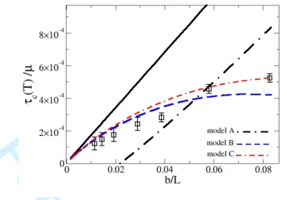
←
−
FIG. 9: Variation of the yield stress versus the Al concentration, computed from the present simulations with different Al random distributions for each concentration (different symbols for each simulation) and different models: Mott-Nabarro statistics for isolated Al (dot-dashed line), for Al pairs (dashed line) and the modified Mott-Nabarro statistics to account for various types of obstacle (continuous line).
1 2 3 4 5 6 7 8 9 10 11 12 13 14 15 16 17 18 19 20 21 22 23 24 25 26 27 28 29 30 31 32 33 34 35 36 37 38 39 40 41 42 43 44 45 46 47 48 49 50 51 52 53 54 55 56 57 58 59 60
For Peer Review Only
D. A model for solid solution hardening at 0 K
In the approximation of a quasi-straight dislocation line (Sec.IV B) where the two partials are rigidly bound, we can now test different models for the hardening of solid solutions at 0 K. In the case of a quasi-straight dislocation (see Eq.30 in Ref.[9]), the yield stress is given by the Mott-Nabarro statistics :
τc= 1 b2(c 2w b f4 m Γ ) 1/3 (2)
with same notation as in Ref.[9], so that Γ = µb2/2, fm = αµb2 and c is the density of obstacles. In Sec.III C, we
calculated the parameters of this formula for different obstacles. However, as one has to account for forces on both partials from various configurations of different obstacles, the formula in Eq.2 is in principle not directly applicable. We propose to extend the Mott-Nabarro statistics to account for obstacles of different nature in interaction with a dissociated dislocation core.
As a first step, we derive a model in case of a quasi-straight undissociated dislocation which interacts with only one type of obstacle. This is the same situation as in Refs.[9, 15], but we proceed differently since we do not make any use of Labush’s method of distribution functions (see Ref.[14] for the original theory and Ref.[15] for its application to dislocation glide in solid solutions). In spite of the fact that our theory is less rigorous than Labush’s one, this will permit us to extend the calculation to a case more complex than the original one.
Let us consider a dislocation which can be separate into segments, the average length of which is Lc. Each segment
corresponds to the wave length of the static wave of our dislocation (see Fig. 8 and Fig. 10). The wavy shape of the dislocation results from the coexistence of regions where the total force is pushing with regions where the total force is retaining the dislocation (see Fig. 10). So this wave length Lc characterizes the solute distribution in the
neighborhood of the dislocation. The difference of density between the pulling and retaining obstacles distributed along the dislocation segment Lc, in a ribbon 2w centered on the average core position, is given by the random
statisticsp2cwLc/s. Here we denoted by s the atomic elementary surface in plane (1¯11): s = 3
√
3b2/8. Since we want to estimate the resistance to the external shear stress, we consider the case where the dislocation is stopped by an excess of retaining obstacles. The total force exerted by the obstacles on the dislocation is: −(Ly/Lc)fmp2cwLc/s.
Submitted to an external shear stress τ , the total variation of enthalpy due to a displacement dx of the dislocation reads dH = τ bLydx − Ly Lc fmdx p 2cwLc/s + δEt, (3)
where δEtis the variation of the energy line tension due to the displacement. We assume that the displacement dx is
small compared to the force range w and that the displacement does not involve a change in distribution forces around the dislocation core. To evaluate δEt, we consider our dislocation as a sine-like string with line tension Γ = µb2/2.
By comparison of the three pictures in Fig. 8, we see that the amplitude of the dislocation bending, denoted by A does not vary significantly with concentration nor with the external stress. On the other hand, one notes that the spatial extension along the dislocation line of the static waves clearly decreases as the concentration increases.
Since one assumes a sine-like shape for the dislocation segment Lc, the retaining and pushing regions have similar
spatial extension. Provided that the dislocation remains pinned by the retaining obstacles, the only parts of the dislocation that can move significantly under the Peach-Kohler force are the regions where the sum of forces is pushing the dislocation. As depicted in Fig. 10, in the region where the obstacles retain the dislocation, the displacement is small compared with the region where the obstacles push the dislocation in the direction of the Peach-Kohler force. In a first order approximation, we neglect the displacement in the region where the obstacles retain the dislocation. During a displacement dx of the average position of the segment Lc, the dislocation displacement in the region where
the obstacles push the dislocation is thus given by 2dx, since the retaining and pushing regions have similar spatial extension. Thus, at the end of the displacement, we have A = Af ≈ A + 2dx. Since the string energy, Et, is given by
(Γ/2)q2A2, where q = 2π/L
c is the wave vector, we obtain:
δEt= Ly Γ(2π)2 2L2 c (A2f − A2) ≈ L y 4Γπ2 L2 c Adx, (4)
to first order in dx. The derivative of the enthalpy variation with respect to dx is, thus to first order in dx:
dH/dx = Ly[τ b − fm p 2cw/(sLc) + 4π2AΓ L2 c ]. (5) 1 2 3 4 5 6 7 8 9 10 11 12 13 14 15 16 17 18 19 20 21 22 23 24 25 26 27 28 29 30 31 32 33 34 35 36 37 38 39 40 41 42 43 44 45 46 47 48 49 50 51 52 53 54 55 56 57 58 59 60
For Peer Review Only
12
FIG. 10: Schematic view of the dislocation (thick line) interacting with a random distribution of obstacles which forces are either pushing or retaining the dislocation. The small arrows indicate the different directions of forces. The notations are defined in text. In the course of an average displacement dx, the dislocation is deformed because of the inhomogeneous force distribution. This leads to an increase of the curvature of roughly 2dx (see text above Eq.4).
The position of the dislocation becomes unstable when dH/dx > 0, which defines the critical stress above which the dislocation glides: τ b = fm p 2cw/(sLc) − 4π2AΓ L2 c . (6)
The segment length Lc depends on the distribution of Al encountered by the dislocation core. The yield stress
corresponds to the maximum of τ with respect to Lc, i.e. when all the dislocation segments of every length Lc can
be released under the stress τ . This maximum value is reached for Lc= L∗c:
L∗c = ( 16π
2ΓA
fmp2cw/s
)2/3 (7)
which decreases as the density of obstacles as expected from the simulations shown in Fig. 8. Combining Eq.6 and Eq.7, and assuming that A ≈ w leads to
τc = 3 8b( c2wf4 m 2π2s2Γ) 1/3, (8)
which gives exactly the same power law as the formula derived by Nabarro in Ref.[9] (see Eq.2), apart from a geometric factor. Eq.8 has also the same form as Mott’s result[8] when A = w = b. A first order development of A as a function of w gives a linear function which the constant term is zero since A must go to zero as w. Indeed, for an external stress that is negligible, when the obstacles are punctual, i.e. w = 0, the dislocation is straight. According to the simulations(Fig. 8), it is reasonable to take A = w. With our notations, Eq.8 may be rewritten as
τc= 3µb 8 ( c2wα4 π2s2 ) 1/3. (9)
We now extend the theory to different types of obstacles and to the dislocation which is dissociated into partials, considered as rigidly bounded. For the quantities fm, α and w, we introduce the subscript i, which represents a single
configuration of a given type in Tab.I, and a subscript j = (1, 2), for the partial which is concerned. The concentration ci is either CAl or CAl2 , since it does not depend on which partial is considered. Along dislocation segment Lc, we
consider the statistics of every type of obstacle such that Eq.5 becomes:
dH = Lydx[τ b − X i,j fm,i,j q 2ciwi,j/(sLc) + 4π2W Γ L2 c ], (10) 1 2 3 4 5 6 7 8 9 10 11 12 13 14 15 16 17 18 19 20 21 22 23 24 25 26 27 28 29 30 31 32 33 34 35 36 37 38 39 40 41 42 43 44 45 46 47 48 49 50 51 52 53 54 55 56 57 58 59 60
For Peer Review Only
where we introduced the quantity W that is the average amplitude of the static wave of the whole core, that is taken as W =P
i,jciwi,j/Pi2ci. The factor 2 at the denominator accounts for the two partials. The line tension Γ is still
given by µb2/2, where b is the total Burgers vector since the partial dislocations are assumed to be rigidly bound.
The coefficients wi,j and αi,j are given in Tab.I. Same arguments as previously developed, lead to the optimal wave
length:
L∗c = ( 16π
2ΓW√s
P
i,jfm,i,jp2ciwi,j
)2/3. (11)
The final formula for the yield stress of a random Al distribution with different types of obstacles is:
τc=
3 8b
(P
i,jfm,i,jp2ciwi,j/s)4/3
(2π2W Γ)1/3 . (12)
This is rewritten within our notations as follows:
τc = 3µb
(P
i,jαi,jp2ciwi,j/s)4/3
8(π2W )1/3 . (13)
The concentration of isolated obstacles is given by ci= CAl− 2CAl2 to avoid the double counting of pairs in the plane
just above the glide plane. For pairs, we have simply ci= CAl2 . The corresponding yield stress is plotted in Fig. 9 as
a continuous line and shows satisfactory agreement with our MS simulations. The length L∗c (Eq.11) varies between 164 b for CAl= 2 % and 7 b for CAl= 10 %. Since Ly> L∗c, the simulation cell is large enough to reduce a possible
size effect due to the fluctuations of the random statistics(App.B). Equation Eq.13 represents an extension of the Mott-Nabarro statistics to the case of various types of obstacle. It is noteworthy that, not only the upward curvature of the yield stress as a function of CAlis well approached by the present expression but even the absolute value of the
yield stress is calculated with good precision without any rescaling factor. Accounting for single solute pinning only would lead to underestimate the yield stress. The results for Mott-Nabarro statistics applied to pairs only is reported in Fig. 9 as a dashed line. The result is closer to our simulations than that for isolated Al. We are thus in a range of concentrations where the pair contribution dominates but both contributions have to be taken into account and properly summed to obtain a good quantitative result. According to Mott-Nabarro statistics applied to pairs only, an exponent 4/3 of the Al concentration can be worked out, replacing c by CAlin Eq.2 or Eq.6. Since the main source
of hardening comes from pair contribution, this exponent, larger than 1, involves the upward curvature of the overall yield stress Eq.13.
In the present development, we did not consider the possibility of Al triplets. In the range of concentrations where such a contribution could dominate that of pairs, a upward curvature should appear clearly since the exponent of CAl
in Eq.2 would be 2. According to the agreement between the simulations and the model presented above, we may reasonably expect that the triplet contribution is not significant in the range of concentrations studied here. At larger concentration in Al, the dislocation pinning of triplets may thus be expected to operate. As we noted for pairs and isolated solutes, the contributions of various cluster size gather to enhance the hardening.
V. TEMPERATURE EFFECT
A. Dislocation dynamics: stop and go motion
Thermal activation is often invoked to explain the unpinning of dislocations when τ < τc. This theory proves
suitable when the activation energy Ea for passing obstacles is much larger than the thermal fluctuations fixed by
kBT , i.e. the time spent at the top of the barrier Ea is negligible in comparison to the occupation of the bottom.
In the case of dislocations under an applied stress τ , the activation energy Ea is defined as E − τ Vact, the difference
between an internal energy barrier E and the work of the Peach-Kohler force which involves an activation volume Vact. In the range of stress-temperature such that Ea/kBT >> 1, the process is thermally activated and it proves
difficult to verify by MD whether the statistics of the activation law applies in such a case. In contrast when Ea/kBT
is of the order of unity, we are able to observe transient arrest periods, which duration δt we call waiting times (see Fig. 12). When the applied stress decreases below the critical stress, and below a value τc(T ), δt becomes larger than
the duration of our simulations. τc(T ) is defined as the finite temperature yield stress of our system.
In his work on solution hardening[15], Nabarro derived a theory to work out the finite temperature yield stress τc(T )
from the zero temperature yield stress τc. As mentioned by Nabarro himself[9], the theory disagrees with experiments.
1 2 3 4 5 6 7 8 9 10 11 12 13 14 15 16 17 18 19 20 21 22 23 24 25 26 27 28 29 30 31 32 33 34 35 36 37 38 39 40 41 42 43 44 45 46 47 48 49 50 51 52 53 54 55 56 57 58 59 60
For Peer Review Only
14
For instance, the power law in concentration does not agree with results on Silver alloys, obtained by Basinski et al. [30]. It would be worth carrying out MD simulations on the thermal activation of the glide process in solid solutions to attempt to improve the theory. This kind of study would require exceedingly long simulations of MD on large simulation cells, so we are not able to present a complete study on that precise point. However, as this proves to be fruitful for the case of zero temperature in Sec.III, our first step is to understand the consequences of thermal fluctuations on the crossing of simple regular chains with periodic condition along Y axis (see Fig. 1). In Fig. 11, we used MD to compute τc(T ) as a function of the distance L between obstacles, for a regular chain of type III obstacles
(see Sec.III). The simulations were performed at 300 K. When the shear stress is large enough, the dislocation is unstopped. The external shear stress has been decreased till the dislocation remains pinned for the duration of our simulations, i.e. a few nano-seconds. Whether a dislocation will move or not depends on the distribution of initial atomic velocities. It is however possible to carry out a statistical treatment over the initial atomic velocities. This results in a distribution of critical stresses rather than a well defined yield stress. Typically 5 independent simulations were performed for each of the 7 values of L depicted in Fig. 11. For a given L, these results are represented as error bars in Fig. 11. We can see that the temperature strongly lowers the resistance of type III Al pair. This decrease is analyzed thoroughly in Sec.V B.
The atomistic processes involved are illustrated in Fig. 12. In our simulation box, we placed 4 pairs of type III (type III, Fig. 4(c)), aligned along the moving dislocation. The distance between the obstacles is fixed to L = 14 b which corresponds to a critical shear stress τc(300K) = 40 Mpa. The detailed atomistic mechanism are followed
by measuring the length of the Al-Al bonds. For τ above τc(T ), the dislocation passes so that the Al pairs follow
the same trajectory and while the crossing they are brought into first neighbor distance. The different stages of the Al-Al bonds length are labelled in Fig. 12(a). Initially the pairs are third neighbors (label A), they becomes second neighbors when the leading partial unpins (B) and then first neighbors (type IV, Fig. 4(d)) when the trailing partial crosses (C). The dislocation makes one loop in the simulation box between (C) and (D), then the leading partial forces the Al atoms to a distance slightly smaller than first neighbors distance. After the second passage of the dislocation, the pairs are again first neighbors (type IV, Fig. 4(e)). Each further dislocation crossing (F) separates the pairs by one b.
When the external stress is slightly below the critical value τc(T ), the dislocation stops (see Fig. 12(b)). As in
Fig. 12(a), we labelled the different stages. Although the two first stages (A and B) are same as in Fig. 12(a), the subsequent evolution differs. The pairs are tentatively put in nearest neighbor positions (C) but eventually return to a second neighbors configuration (D). The latter is preferred to the former because of the repulsive character of the Al-Al interaction in the core of the dislocation. It is noteworthy that the bond length of the 4 independent pairs have been plotted in the same figures Fig. 12(a) and Fig. 12(b). The different plots are superposed so that they are hardly distinguishable which shows that the pairs flip simultaneously and that the dislocation crosses coherently the chain of obstacles.
For an applied stress between τc(T ) and τc, the dislocation may stop for a waiting time that decreases sharply as
the shear stress increases and falls to an extremely low value when the shear stress is larger than τc.
B. Models for temperature effect
We propose different models for the temperature effect on the crossing of simple regular chains. First, we us denote by f (x) the force sustained by the dislocation due to the presence of obstacles in its course. At equilibrium, τ bL + f (x) = 0 where x is the distance between the obstacle and the partial which interacts significantly, and L is the distance that separates two neighboring obstacles. The distance x is the same for all periodic images of the obstacle. We develop f (x) around its maximum (xm):
f (x) = fm+ 1/2
d2f
dx2(xm)(x − xm) 2
. (14)
At a distance corresponding to the range of the interaction w, as estimated in Sec.III C, we can estimate that f (xm± w) ≈ 0, thus d2f /dx2(xm) = −2fm/w2. The force has then a quadratic form. Furthermore the yield stress is
such as fm= −τcbL. Consequently, the equilibrium is given by:
(τ − τc)bL +
τcbL
w2 (xeq− xm)
2= 0 (15)
The stable equilibrium position is:
xeq= xm− w p (τc− τ )/τc. (16) 1 2 3 4 5 6 7 8 9 10 11 12 13 14 15 16 17 18 19 20 21 22 23 24 25 26 27 28 29 30 31 32 33 34 35 36 37 38 39 40 41 42 43 44 45 46 47 48 49 50 51 52 53 54 55 56 57 58 59 60
For Peer Review Only
FIG. 11: Critical shear stress of a regular chain of type III obstacles spaced by L at 300 K (square symbols) and at 0 K (full line).
Integrating the total force τ bL + f (x) between the equilibrium position xeq and the limit of stability xm gives the
total work W one must provide to overcome the potential barrier:
δW = −2b 3 Lwτ
−1/2
c (τc− τ )3/2. (17)
We assume that the whole dislocation moves coherently (which is confirmed by the simulations in Sec.V A). From the bottom of this potential, i.e. x = xeq, to overcome the barrier, the kinetic energy of the dislocation core, Ec must
rise by −δW . The initial kinetic energy of each atom along the X direction is, on the average kBT /2, which gives a
thermal energy per unit length of dislocation kBT /(2b
√
3), where b√3 is the distance between two atoms along the dislocation line. Assuming that the thermal fluctuations are optimally distributed to pass the barrier, we obtain the yield stress at finite temperature:
τc(T ) = τc− (
3kBT
4√3b2w) 2/3
τc1/3. (18)
It is worth noting that this formula shows a power 2/3 of temperature, similar to the theory proposed by Nabarro in Ref.[9] for thermal effect on solid solution hardening. However, in our case of a regular obstacle chain, the difference (τc − τc(T )) is proportional to τ
1/3
c whereas for solid solutions a τ 2/3
c is expected[9]. Since the exponent of τc is
less than 1, there is a boundary value of τc below which τc(T ) becomes negative and thus the predicted hardening
becomes negligible. This boundary increases as the power 2/3 of temperature. Eq.18 is plotted versus 1/L in Fig. 11 (labelled by A, dot-dashed line). Clearly, this model fails to reproduce the numerical simulations. The discrepancy probably stems from the assumption that the thermal activation of the dislocation is associated with a rigid body motion. One has to account for the finite line tension and the fluctuations in shape of the dislocation to describe more accurately the thermal activation process. In order to do so we assume that the free segments of the dislocation trailing partial can be approached by a string which oscillates around an equilibrium position as stationary waves of amplitude A (see Fig. 13). The X component of the total force exerted on the pinned point of the dislocation line is Fp = τ bL − τcbL + N where the first term is the Peach-Koehler force, the second term is the maximum of the
obstacle force and the third one is due to fluctuations of the line tension. Assuming a sine form for the dislocation wave and denoting by A the amplitude of oscillations and qn = nπ/L the wave momentum with mode number n,
then the maximum force due to the line tension projected on X is N = 2qnAΓ. According to the standard oscillating
string theory, the vibration energy of the mode n is Lyq2nA2Γ/2 which is assumed to reach kBT /2 at thermodynamical
equilibrium of the segment. The total force Fp is zero when τ reaches τc(T ) that is:
τc(T ) = τc− 2/b p kBT × Γ/L3. (19) 1 2 3 4 5 6 7 8 9 10 11 12 13 14 15 16 17 18 19 20 21 22 23 24 25 26 27 28 29 30 31 32 33 34 35 36 37 38 39 40 41 42 43 44 45 46 47 48 49 50 51 52 53 54 55 56 57 58 59 60
For Peer Review Only
16
FIG. 12: Time evolution of the distance between Al pairs in a regular chain made of 4 independent pairs separated by 35˚A, at different external shear stress τ , e.g. τ = 60 MPa in (a) and τ = 30 MPa in (b). See the text for a detailed description of the various sequences.
(a)
(b)
As the unpinning of the second partial is the controlling reaction Γ is here given by Γ = µb2
p/2 where bp≈ b/2. Since
τc= αµb/L, Eq.19 can be rewritten as:
τc(T ) = τc−
2τc3/2
b p
kBT × Γ/(αµb)3. (20)
We note that the temperature exponent in Eq.20 is 1/2 whereas it was 2/3 in Eq.18. The exponent of τcin the second
term at the right hand side in Eq.20 is now larger than 1, by contrast to Eq.18. Consequently, the predicted τc(T )
in Eq.20 remains positive for small values of τc. The variation of the theoretical critical stress predicted by Eq.20
is plotted in Fig. 11 (labelled by B, dashed line) and proves to be in good agreement with the simulation results indicating that the oscillating string model captures the physics of thermally activated unpinning of the dislocation in interaction with a regular array of obstacles. The agreement can be improved by adjusting the value of the partial line tension Γ upon atomic simulations in order to take into account the effect of the dissociated core[31]. A rescaling
1 2 3 4 5 6 7 8 9 10 11 12 13 14 15 16 17 18 19 20 21 22 23 24 25 26 27 28 29 30 31 32 33 34 35 36 37 38 39 40 41 42 43 44 45 46 47 48 49 50 51 52 53 54 55 56 57 58 59 60
For Peer Review Only
FIG. 13: Schematic representation of the dislocation deformation when it is pined onto a regular chain of obstacles made of Al pairs of type III. The coefficient A denotes the amplitude of the stationary wave sustained by the pined partial, i.e. the trailing one.
of 80 % of the line tension allows to obtain the plot corresponding to label (C) in Fig. 11. For small value of L in Eq.19 (i.e, large τc in Eq.20), τc(T ) can be negative which indicates a drawback of the model that is ascribed to the
fact that the dislocation cannot be considered as an oscillating string when the obstacles are close from each other. The combination of the rigid string model (model (A)) and of the oscillating string model (model (B)) might allow to improve our approach of the temperature effect. The nucleation of thermally activated double kinks to pass the Al barrier could also be a possibility. In the case of not too small spacings between obstacles, the agreement between the simulations and the oscillating string model shows that it is surely the fluctuations of the dislocation line which operates the unpinning. In this case, it is noteworthy that the stronger the obstacle chain the larger the softening due to the temperature. Hence the effect of Al dimers is expected to be more attenuated than that of isolated solutes. Such a softening of the strongest obstacles could involve a change in the dislocation glide statistics as a function of the temperature.
VI. DISCUSSION
Atomistic simulations shed a new light on the problem of solute hardening[7] in which F.R.N. Nabarro has made major contributions. The complexity of developing reliable inter-atomic potentials for alloys postpone to the future the direct application of these simulations to a variety of solid solutions. However this approach can guide in the understanding of the atomistic aspects which cannot be accounted for by the classical elastic theories. The main finding of our paper is that solute pairs, whether they cross the glide plane or not, play a dominant role in hardening concentrated solid solutions; this reflects into the variation of the yield stress as function of solute concentration. The pair contribution is enhanced by the various possibilities of the bond direction. We have also demonstrated how to take advantage of such simulations to address the still open problem of the thermal activation of dislocation motion in a solid solution. The computer simulations described here can be seen as sophisticated thought experiments which helped us to generalize Mott-Nabarro model for solid solution hardening: the extension we propose, accounts for the effect of atom pairs and attempts to incorporate thermal activation effects. Since the computer simulations depend obviously on the inter-atomic potentials, our results need to be confirmed in different situations, i.e. different potentials and different systems.[32] A comparison with experiments proves difficult because of the low solubility limit in the solid solutions similar to Ni(Al). By way of contrast in the computer simulations, the diffusion process of the solute can be ignored because the simulation time scale is much smaller than the jump rate of defects. This allowed us to address properly the case of one dislocation in a single monocrystal of purely random solution. In the experiments, the presence of the grain boundaries, other impurities or other dislocations may impede the analysis of the solid solution hardening.
The phenomena identified in this paper pinpoint two main issues which should not be overlooked: the importance of chemical bonds in concentrated solid solutions, and the role of the detailed local crystallography. One can expect
1 2 3 4 5 6 7 8 9 10 11 12 13 14 15 16 17 18 19 20 21 22 23 24 25 26 27 28 29 30 31 32 33 34 35 36 37 38 39 40 41 42 43 44 45 46 47 48 49 50 51 52 53 54 55 56 57 58 59 60
For Peer Review Only
18
for instance that short range order hardening could be explored along the same lines, and the case of solute hardening in bcc metals, still largely unsolved, should also benefit from these approaches in a near future.[33]
[1] R. Phillips, Crystals, Defects and Microstructures: Modeling Across Scales, (Cambridge University Press, 2001). [2] S. Yip, Handbook of Materials Modeling, (Springer Netherland, 2005).
[3] R. Madec, B. Devincre, L. Kubin, T. Hoc and D. Rodney, Science 301, 1879 (2003). [4] V. Vitek, Crystal Lattice Defects 5, 1 (1974).
[5] V. Yamakov, D. Wolf, S. R. Phillpot, A. K. Mukherjee and H. Gleiter, Nature Materials, 45 (2002). [6] S. J. Zhou, D. L. Preston, P. S. Lomdahl, D. M. Beazley, Science 279, 1525 (1998).
[7] N. F. Mott and F. R. N. Nabarro, Report on Strength of Solids, (London: The Physical Society, 1948) pp. 1-19.
[8] N. F. Mott, Imperfections in Nearly Perfect Crystals, Ed. by W. Shockley, J. H. Holomonn, R. Maurer and F. Seitz (New York: John Wiley, 1952), pp. 173-190.
[9] F. R. N. Nabarro, in ”Dislocations and Properties of Real Materials” (London, The Institute of Metals, 1985), p. 152. [10] J. Friedel, Les Dislocations, (Gauthier-Villars, Paris, 1956) p. 205.
[11] E. Rodary, D. Rodney, L. Proville, Y. Br´echet, and G. Martin, Phys. Rev. B 70, 054111 (2004).
[12] P. Haasen, in Dislocations in Solids, edited by F.R.N. Nabarro (North-Holland, Amsterdam, 1979), Vol. 4, p. 155. [13] Th. Wille, G. Gieseke and Ch. Schwink, Acta Metall. 35, 2679 (1987).
[14] R. Labush, Phys. Status Solidi 41, 659 (1970).
[15] F. R. N. Nabarro, Journal of the Less-Common Metals 28, 257 (1972). [16] J. Friedel, Dislocations, (Addison-Wesley, 1964) p. 224.
[17] U.F Kocks, A. Argon, M. Ashby, Thermodynamics and Kinetic of slip, Progress in Material Science, (1975) p. 60. [18] B.R. Riddhagni and R.M. Asimow, J. Appl. Phys. 39 4144 (1968). ibid, 5169.
[19] Pr. F.R. Nabarro is gratefully acknowledged for this remark made to one of us, GM. [20] P. Jax, P. Kratochvil and P. Haasen, Acta Metall. 18, 237 (1970).
[21] J.E. Angelo, N.R. Moody and M.I. Baskes, Modell. Simul. Mater. Sci. Eng. 3, 289 (1995). [22] D. Rodney and G. Martin, Phys. Rev. B 61, 8714 (2000).
[23] C.B. Carter and S.M. Holmes, Phil. Mag. 35, 1161 (1977).
[24] A.F. Voter and S.P. Chen, Mater. Res. Soc. Symp. Proc. 82, 175 (1987). [25] F. Ercolessi and J.B. Adams, Europhys. Lett. 26, 583 (1994).
[26] The table Tab.I summarizes the nature of obstacles, the manner they interact with the dislocation, their interaction coefficients α and the force range w.
[27] R.L. Fleisher, Acta Metal. 11, 203 (1963); in The Strengthening of Metals, edited by D. Peckner, Reinold Press Edition, 1964, p. 93.
[28] J. P. Hirth and J. Lothe, Theory of dislocations, (Wiley Interscience, 1982) p. 507. [29] A. H. Cottrell, Dislocations and Plastic Flow in Crystals, (Clarendon Press, Oxford, 1953). [30] Z.S. Basinski, R.A. Foxall and R. Pascual, Scripta Metall. 6, 807 (1972).
[31] K. Hardikar, V. Shenoy and R. Phillips, Journal of Mechanics and Physics of Solids 49, 1951 (2001). [32] D.L. Olmsted, L.G. Hector Jr, W.A. Curtin and R.J. Clifton, Modelling Simul. Mater. Sci. Eng. 13, 371
(2005).
[33] K. Tapasa, D.J. Bacon and Yu. N. Osetsky, Materials Science and Engineering A 400, 109 (2005).
1 2 3 4 5 6 7 8 9 10 11 12 13 14 15 16 17 18 19 20 21 22 23 24 25 26 27 28 29 30 31 32 33 34 35 36 37 38 39 40 41 42 43 44 45 46 47 48 49 50 51 52 53 54 55 56 57 58 59 60
For Peer Review Only
Symbols Meaning value
a0 Ni lattice parameter 3.52 ˚A
b norm of Burgers vector for a edge dislocation b = a0/
√ 2 bp edge part of partial Burger vectors b/2
µ Ni shear modulus in (1¯11) 74600 MPa
v Ni atomic volume 11 ˚A3
vs Al atomic volume 16.6 ˚A3
TABLE II: Notations and values of our constants.
Symbols Meaning
α pinning strength normalized with respect to µb2
β Labush factor
βel coefficient of the hydrostatic work
fm obstacle force
L nearest neighbor distance between obstacles Lc dislocation core wave length in a distribution of obstacles
L∗c dislocation core wave length in the strongest distribution of obstacles
ni number of significant obstacles of type i = (I, II, III, IV )
τ resolved external shear stress
τc yield stress at 0 K
τc(T ) critical shear stress at temperature T
w range of obstacle force
TABLE III: Notations of our variables.
APPENDIX A: NOTATIONS
Our notations for constants and variables are resumed in tables Tab.II and Tab.III, respectively.
APPENDIX B: SIZE EFFECTS IN SIMULATION OF A SOLID SOLUTION
The size effects in solid solution simulations are mainly due to our finite size along the dislocation line, i.e. in the Y direction, Ly. This involves interactions between the dislocation and the solutes and their periodic images along Y
which may artificially pin the dislocation. As it is seen in Sec.III B, according to our calculations, the pinning effect of a regular chain becomes negligible compared to the yield stress of our solid solutions, whenever the obstacle spacing is larger than 100 times the Burgers vector. One could thus have fixed our box size along Y to 100 b but a more subtle size effect has a different origin than the interaction between periodic images.
The number of obstacles (isolated Al atoms or pairs of Al) is denoted by No. As we assume the purely random
disorder, the fluctuation of this number is ∆o =
√
No. The random statistics is satisfactorily represented to the
condition that ∆o<< No. If this condition is not satisfied, then our dislocation may encounter an abnormally high or
low concentration of obstacles either an excess or a lake of√No/2. The size effect on the statistics is tightly related
to the characteristics of the interactions between the obstacles and the dislocation. The number of partials concerned as well as the obstacle density and the range of the interaction should be involved in the estimation of the required size. In order to account for these features, a model is proposed in Sec.IV D. According to this model, the scale of the statistical fluctuations along the dislocation line, L∗c is smaller than the size of the simulation cell along Y direction. We can thus reasonably expect that the inequality ∆o<< Nois verified.
To reach the large Y sizes, we have reduced the dimensions in the other directions and particularly in the X direction. The size Lxis only 10 times larger than the separation width between partials which could involve elastic
interactions between the core dislocation and its periodic images along X. However the distance between periodic images is still 100 b, which is larger than the distance between the dislocation core and the solute atoms in solid solutions. The interaction between dislocation core and the solute atoms is thus expected to dominate the possible interactions between the core dislocation and its periodic images along X direction.
1 2 3 4 5 6 7 8 9 10 11 12 13 14 15 16 17 18 19 20 21 22 23 24 25 26 27 28 29 30 31 32 33 34 35 36 37 38 39 40 41 42 43 44 45 46 47 48 49 50 51 52 53 54 55 56 57 58 59 60