HAL Id: hal-01295061
https://hal.inria.fr/hal-01295061
Submitted on 30 Mar 2016
HAL is a multi-disciplinary open access
archive for the deposit and dissemination of
sci-entific research documents, whether they are
pub-lished or not. The documents may come from
teaching and research institutions in France or
abroad, or from public or private research centers.
L’archive ouverte pluridisciplinaire HAL, est
destinée au dépôt et à la diffusion de documents
scientifiques de niveau recherche, publiés ou non,
émanant des établissements d’enseignement et de
recherche français ou étrangers, des laboratoires
publics ou privés.
Parallelizing Constraint Solvers for Hard RCPSP
Instances
Roberto Amadini, Maurizio Gabbrielli, Jacopo Mauro
To cite this version:
Roberto Amadini, Maurizio Gabbrielli, Jacopo Mauro. Parallelizing Constraint Solvers for Hard
RCPSP Instances. [Technical Report] Inria Sophia Antipolis. 2016. �hal-01295061�
Parallelizing Constraint Solvers for
Hard RCPSP Instances
?Technical Report
Roberto Amadini1,2, Maurizio Gabbrielli1,2, and Jacopo Mauro3
1
Department of Computer Science and Engineering, University of Bologna, Italy.
2
FOCUS Research Team, INRIA, France.
3
Department of Informatics, University of Oslo, Norway.
Abstract. The Resource-Constrained Project Scheduling Problem (RCPSP) is a well-known scheduling problem aimed at minimizing the makespan of a project subject to temporal and resource constraints. Constraint Programming allows to model and solve RCPSPs in a natural and efficient way, especially when Lazy Clause Generation (LCG) techniques are employed. In this paper we show that hard RCPSPs can be efficiently tackled by a portfolio approach that combines the strengths of different —not necessarily LCG-based— solvers by exploiting their parallel execution on multiple cores. Our approach seeks to predict and run the best solvers for a new, unseen RCPSP instance and also enables the bounds communication between them. This on-average allows to outperform the oracle solver that always chooses the best available solver for any given instance.
1
Introduction
The Resource-Constrained Project Scheduling Problem (RCPSP) [9] is the problem of minimizing the makespan (i.e., the total duration) of a project, defined as a collec-tion of tasks subject to precedence relacollec-tions between the activities and constrained by resource availabilities. This well-known NP-hard problem [8] has countless industrial applications and it is one of the most studied scheduling benchmark.
The Constraint Programming (CP) [30] paradigm allows to model and solve hard combinatorial problems. In particular, RCPSP can be naturally and elegantly encoded into a Constraint Optimization Problem (COP) where: (i) integer variables are used to track the start time of each task; (ii) constraints over such variables ensure compliance with the precedence relations and resource capabilities; (iii) a special integer variable keeps track of the makespan. The goal is to find an optimal solution, i.e., a consistent assignment of the variables which minimizes the makespan.
An effective technique for solving CP problems consists in using Lazy Clause Gen-eration(LCG) [28] techniques. The key idea of LCG is to mimic the Finite Domain propagation by properly generating corresponding SAT clauses during the search. LCG can significantly boost the search for many combinatorial problems, including RCPSP
?
Supported by the EU project FP7-644298 HyVar: Scalable Hybrid Variability for Distributed, Evolving Software Systems.
and its variants, but obviously it is not a panacea and there are cases in which LCG is not fruitful.
To exploit the diverse nature and performance of different solving techniques, a fairly recent trend consists in using a portfolio approach [14]. Basically, given a portfo-lio {s1, . . . , sm} of m > 1 solvers, a portfolio solver seeks to predict the best solver(s)
si1, . . . , sik (with 1 ≤ ij ≤ m for j = 1, . . . , k) for solving a new, unseen problem
p and then runs such solver(s) on p. In this context, scheduling k > 1 solvers can re-duce the risk of selecting only one solver —maybe a bad one for p— and especially enables the knowledge sharing between the scheduled solvers, as well as their parallel execution. Surprisingly, despite their effectiveness, portfolio solvers have been poorly adopted in real-life applications.
In this work we join the aforementioned research streams by showing how CP can be successfully applied for solving hard RCPSP instances by means of a parallel portfolio approach. We first retrieved a fairly large number of non-trivial RCPSPs encoded in MiniZinc[26], nowadays one of the most widely used language to define COPs. We then defined some variants of the parallel portfolio solver sunny-cp [3], the gold medalist in the open category of MiniZinc Challenge 2015 [34, 35], to boost the resolution of the RCPSP instances.
We would like to underline that this is not a “standard” application of a portfolio approach because in this case there is a dominant solver (the LCG solver Chuffed [12], publicly available at [11], best solver of the MiniZinc Challenges 2012—2015 in the free search category) which is able to greatly outperform all the other solvers. This set-ting is not unusual in many real-life applications. For instance, companies are typically interested in solving only a specific kind of problem emerging from the business pro-cess. Conversely, this scenario is not so common in the benchmarks used for evaluating portfolios since the effectiveness of a portfolio approach relies on the diversity of good solvers.
The emphasis of this work is not on the Algorithm Selection problem [23,29] where we are only interested in predicting the best solver for a given problem. Here we show instead how it is possible to combine, leverage, and run simultaneously the predicted solvers on RCPSPs to outperform the best available solver and to be on-average better than the Virtual Best Solver, i.e., the oracle solver that always chooses the best solver for any given RCPSP instance (or, equivalently, that always runs simultaneously all the available solvers of the portfolio without synchronization and memory contention issues).
Furthermore, we remark that the focus of this work is not on sunny-cp tool. Conversely, here we are interested in advancing the state of the art of CP techniques for solving difficult RCPSPs problems. In particular, we show that state-of-the-art LCG solvers can be significantly overcome thanks to other constraint solvers not employing LCG. The message of the paper is twofold: (i) we prove that the belief that portfolios can not be applied in real-life scenarios characterized by a dominating solver is false, (ii) we show that by parallelizing the solvers execution and by enabling the bounds communication between the scheduled solvers we can get an overall better solver which is even greater than the sum of its parts. To the best of our knowledge, we are not aware of similar approaches for efficiently solving hard RCPSP instances.
Paper Structure.Section 2 gives background notions about RCPSP and sunny-cp. In Section 3 we explain the evaluation methodology. Section 4 reports the experimental results, while Section 5 draws concluding remarks.
2
Background
In this section we give some background notions about the RCPSP problem and the sunny-cpportfolio solver.
2.1 RCPSP
The RCPSP resolution has attracted a lot of attention over the last decades, since this problem emerges from many real-life scenarios. For this reason, several formulations and techniques have been proposed for efficiently solving RCPSP and its variants [15, 16, 21]. The most effective methods make use of hybrid approaches that combine the effectiveness of modern SAT solvers with other solving techniques such as Finite Do-main propagation or Linear Programming [17,31,32]. To the best of our knowledge, the LCG approach gives the best results for RCPSP [32] and variants like RCPSP/max [33] and RCPSP/max-cal [24].
In this paper we examine a possible CP formulation of RCPSP, as it appears in MiniZinc 1.6 benchmarks,4 and we show how state-of-the-art solvers based on LCG techniques can be significantly overcome by taking advantage of a portfolio of con-straint solvers not necessarily employing LCG.
The model we consider consists of: – a set of resources R = {r1, . . . , rm};
– a set of tasks T = {t1, . . . , tn};
– a set of precedences between tasks P = {P1, . . . , Pn}, such that Pi ⊆ T \ {ti}
contains the successors of tasks ti.
Each resource rjhas a fixed capacity cj ∈ N, and each task tirequires a fixed capacity
qi,j∈ [0, cj] of resource rj. Each task tihas a constant duration di∈ N over time. The
objective is to find an optimal schedule, i.e., a function σ : T → N such that: – σ(ti) is the starting time of ti;
– σ meets all the precedence and capacity constraints;
– the makespan, defined as max{σ(ti) + di| i = 1, . . . , n}, is minimal.
The model is already annotated with a default search strategy imposing to first select the variable having smaller domain (i.e., the min-dom heuristic) and then try to assign to such variable the smaller value of its domain (min-value heuristic). The study of alternative heuristics is outside the scope of this paper and left as future work.
4
Available at https://github.com/MiniZinc/minizinc-benchmarks/blob/ master/rcpsp/rcpsp.mzn
2.2 sunny-cp
sunny-cpis an open-source portfolio solver. While its first implementation was se-quential [4], its current version exploits multicore architectures for running more solvers simultaneously by exploiting their cooperation via bound sharing and restarting poli-cies. sunny-cp won the gold medal in the open category of MiniZinc Challenge 2015 and, to the best of our knowledge, it is currently the only parallel portfolio solver able to solve generic COPs. A detailed explanation about sunny-cp can be found at [3]. Here we briefly recall how it works.
sunny-cpis built on top of SUNNY algorithm [2] taking a fixed solving timeout T and portfolio Π. SUNNY exploits the k-Nearest Neighbours (k-NN) algorithm to produce a sequential schedule σ = [(s1, t1), . . . , (sk, tn)] where solver si ∈ Π has
to be run for ti seconds andPni=1ti = T . Then, σ is parallelized on the c available
cores. The first and most promising c − 1 solvers are allocated to the first c − 1 cores, while the remaining solvers are assigned to the last available core by linearly widening their allocated times for covering the whole time window [0, T ]. In the particular case of RCPSPs, the most promising solvers are those that are faster in finding the minimal makespan values in the k-neighborhood.
Solvers are run in parallel and a “bound-and-restart” mechanism is used for en-abling the bounds sharing between the running solvers. This allows to use the (sub-optimal) solutions found by a solver to narrow the search space of the other scheduled ones. Since sunny-cp treats solvers as black boxes, it does not support the knowledge sharing without their interruption. Therefore, a restarting threshold Tris used to decide
when to stop a solver and restart it with a new bound. A running solver is stopped and restarted if it has not found a solution in the last Trseconds and its current best bound
is obsolete w.r.t. the overall best bound found by another scheduled solver.
sunny-cpsolves problems encoded in the MiniZinc language [26]. By default, it uses a portfolio Π of 12 state-of-the-art solvers disparate in their nature (viz., Chuffed, CPX, G12/CBC, G12/FD, G12/LazyFD, G12/Gurobi, Gecode, MinisatID, Choco, Ha-ifaCSP, iZplus, and OR-Tools). Some of them are provided in two variants: fixed and free. The fixed variant is optional, and forces a solver to use the search strategy pos-sibly defined in the MiniZinc input model. The free variant instead allows a solver to use its preferred search strategy, ignoring any other search annotation that appears in the MiniZinc model. By default, in line with what most of its constituent solvers do, sunny-cpuses the fixed variant of a solver (when provided) to exploit the domain knowledge of who wrote the MiniZinc model. However, as later detailed, the free vari-ant may significvari-antly outperform the fixed one and should be taken into account when solving a problem.
3
Experiments Methodology
The RCPSP model described in Section 2.1 is the most represented problem class in the MiniZinc 1.6 benchmarks with 2904 RCPSP instances coming from different scenarios [1, 6, 10, 22, 25, 27]. However, most of these instances are not challenging: often the best solvers of sunny-cp can solve them in a matter of seconds. These instances are
not so interesting since a pre-solving that statically schedules the best solvers for few seconds can solve them without any prediction. For this reason we focus our attention on the “hardest” RCPSP instances of the benchmark. After running both the fixed (when available) and free version of the constituent solvers of sunny-cp with a time limit of T = 900 seconds,5we discarded all the instances for which at least one solver was
able to prove the optimality of a solution (or the problem unsatisfiability) in less than T /10 = 90 seconds. In this way we obtained a dataset ∆ of 647 RCPSPs for each of which at least one solver of the portfolio is able to find a feasible solution.
Let U be a universe of solvers and T a solving timeout. To measure the performance of solver s ∈ U —whether it be an individual or a portfolio solver— on a problem instance p ∈ ∆ within T seconds, we consider the following three metrics:
– OPT: measures the optima proven. If s proves the optimality of a solution for p, then OPT(s, p) = 1; otherwise, OPT(s, p) = 0;
– TIME: measures the optimization time. If s proves the optimality of a solution for p in t < T seconds, then TIME(s, p) = t; otherwise, TIME(s, p) = T ;
– OBJ: measures the quality of a solution, by normalizing its makespan value in range [0, 1]. If s finds no solution, then OBJ(s, p) = 0. Otherwise, if mkspan(s, p) is the best makespan found by s for problem p and Mp = {mkspan(s, p) | s ∈ U } is
the set of the best makespans for all the solvers of U , then: OBJ(s, p) = 1 −mkspan(s, p) − min Mp
max Mp− min Mp
.
In this way, the better the makespan the higher is OBJ. In particular, we have that OBJ(s, p) = 1 if and only if s finds the best solution in U for p.
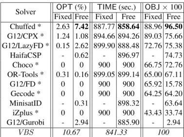
Table 1 shows the average performance of the individual solvers of sunny-cp, with the exception of G12/CBC that was not used due to its very poor performance. We added as baseline the Virtual Best Solver (VBS ), the oracle portfolio solver that —for a given problem and performance metric— always chooses the best solver in the portfolio.6 The VBS is a standard baseline used for evaluating the performance of a
portfolio approach and usually the desired goal is to get as close as possible to the VBS performance.
As can be seen, for almost 90% of the dataset ∆ (578 instances) no solver is able to prove the optimality in 900 seconds. Chuffed clearly dominates all the other solvers, almost reaching the VBS performance. In particular its free version turns out to be very effective. This is probably due to the decision heuristics it uses in its free version, e.g., the Variable State Independent Decaying Sum (VSIDS) [13] heuristic. The effective-ness of LCG is also confirmed in Table 1 by the performance of the others LCG-based solvers, namely CPX and LazyFD.
Note that —depending on the solver and the evaluation metric— using the free search is not always the best choice. Given the diversity of the results by considering different search strategies, we decided to test three different variants of sunny-cp:
5
900 seconds was the timeout of MiniZinc Challenge 2014.
6The VBS of a portfolio Π can be seen as a parallel solver that run simultaneously all the |Π|
solvers without synchronization and memory contention issues (and without bounds commu-nication).
Solver
OPT (%)
TIME (sec.)
OBJ × 100
Fixed Free Fixed
Free
Fixed Free
Chuffed *
2.63 7.42 887.77 858.64 88.96 96.50
G12/CPX *
1.24 1.08 894.66 894.26 89.03 75.66
G12/LazyFD * 0.15 2.62 899.90 888.48 72.76 75.38
HaifaCSP
-
0.62
-
896.97
-
74.73
Choco *
0
0
900
900
66.75 72.76
OR-Tools *
0.31 0.16 899.05 899.14 65.00 67.11
G12/FD *
0
0
900
900
65.92 15.78
Gecode *
0
0
900
900
64.25 64.20
MinisatID
-
0.31
-
898.32
-
63.64
iZplus *
0
0
900
900
43.43 33.74
G12/Gurobi
-
2.94
-
885.90
-
2.94
VBS
10.67
841.33
100
Table 1. Average solvers performance. The fixed version is available only for the solvers marked with *. Peak performances are highlighted in bold.
– sunny-def: the default version of sunny-cp. It uses the portfolio Πdef of the
11 solvers listed in Table 1 by always considering the fixed version of a solver when available;
– sunny-all: uses a portfolio Πallof 11 + 8 = 19 solvers which extends Πdef by
including all the versions of all the available solvers;
– sunny-stc: uses a variable sized portfolio Πc,µof c solvers, where c is the
num-ber of available cores and µ ∈ {OPT, TIME, OBJ} is a performance measure. Specifically, Πc,µis the subset of the best c solvers of Πallaccording to the average
value of µ over dataset ∆.
sunny-allis the natural extension of sunny-def, which allows to measure the impact of adding the free versions of solvers to the default portfolio. Both sunny-all and sunny-def are dynamic approaches, since they select the solvers to run on-line according to the instance to be solved. sunny-stc follows instead a static approach. Indeed, since for each number of cores c its portfolio Πc,µ contains exactly c solvers,
no prediction is performed and all its solvers are launched simultaneously regardless of the instance to be solved. sunny-stc allows to investigate to what extent the solvers prediction of sunny-all is really fruitful and to understand the marginal contribution of the solvers belonging to Πall\ Πc,µ.
There are clearly many different variants of sunny-cp that might be considered. We also tested other plausible sunny-cp variants (e.g., by switching the free/fixed search strategy every time a solver is restarted). These however did not lead to major benefits. Clearly, an exhaustive evaluation of all of the variants is a daunting task due to the combinatorial explosion of all the possible approaches and to the fact that a single test on all the RCPSPs of ∆ requires on average more than 150 computation hours. Following a standard practice for avoiding biasing and overfitting, we validated our
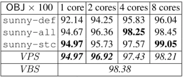
OBJ × 100 1 core 2 cores 4 cores 8 cores
sunny-def
92.14 94.25
95.83
96.04
sunny-all
94.67 96.36
98.25
98.45
sunny-stc
94.97 95.73
97.57
99.05
VPS
94.97 96.92
97.43
98.21
VBS
98.38
Table 2. OBJ performance.
experiments by using a 10-fold cross-validation [5]. We partitioned the dataset ∆ in 10 subsets ∆1, . . . , ∆10called folds, treating in turn a fold ∆ias the test set and the union
S
j6=i∆j of the other folds as the training set. For all the sunny-cp approaches, we
kept the default value Tr= 5 seconds for the restarting threshold. Since sunny-cp is
parallel, we ran the three versions of sunny-cp by considering 1, 2, 4, and 8 cores.
4
Results Discussion
This Section discusses in detail the performance of sunny-def, sunny-all, and sunny-stcin terms of OBJ, OPT, and TIME when exploiting a different number of cores. In addition to the VBS we also introduced the Virtual Parallel Solver (VPSc,µ),
an oracle portfolio solver that for c ∈ {1, 2, 4, 8} and µ ∈ {OPT, TIME, OBJ} simu-lates the parallel and independent execution of the solvers of the portfolio Πc,µ
intro-duced in Section 3. For simplicity, where there is no ambiguity, we will use the notation VPS or VPSc instead of VPSc,µ. We recall that VBS and VPS are “virtual” since
they are not implemented but simulated according to the solvers performance on ∆. Since by definition VPS is a bound of the performance of sunny-stc approach with-out bounds communication and synchronization overheads, the VPS baseline allows to measure the effectiveness of bounds communication. Note also that with this definition the Single Best Solver (SBS ) of the portfolio (i.e., the free version of Chuffed) is equiv-alent to the VPS1and the sunny-stc approaches when using a single core (c = 1)
since Π1,µ = {Chuffed/Free} for every µ ∈ {OPT, TIME, OBJ}. Furthermore, the
VBS is equivalent to VPS|Πall|.
4.1 OBJ Results
Considering the OBJ metric we can say that most of the sunny-cp approaches pro-vide high quality solutions (0.95 < OBJ < 1) even when optimality is not proven. Table 2 shows that the demarcation between the different approaches is not so sharp since SBS is very close to VBS (see Table 1).7
The only approach that performs rather poorly is sunny-def when exploiting just one core. However, we remark that this approach contains only the fixed versions of the
7Note that the OBJ values of the SBS and VBS of Table 1 differ from those of Table 2, since
introducing sunny-cp in the universe U allowed to find new and better makespan values, thus reducing the average OBJ of SBS and VBS .
sunny-def sunny-all sunny-stc 0 20 40 60 80 100 120 140 160 180
1 core 2 cores 4 cores 8 cores
N o . o f in s ta n c e s
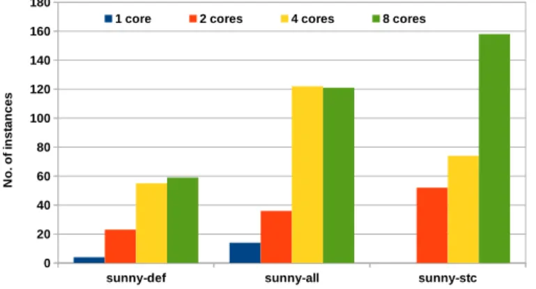
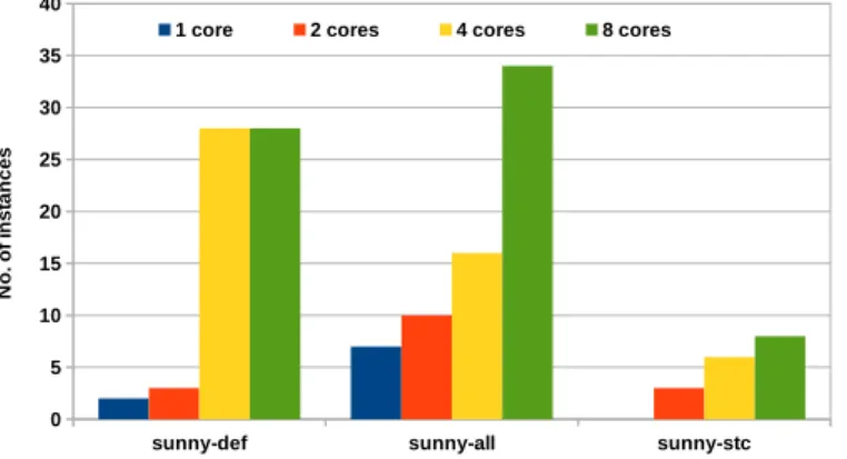
Fig. 1. Number of times sunny-cp outperforms the VBS in terms of OBJ.
solvers: if we add the free versions to the portfolio we can see a clear OBJ improve-ment (from the 92.14 of sunny-def to the 94.67 of sunny-all). Unfortunately, with c = 1 core Chuffed/Free is still better (94.97). This means that the solvers pre-diction is not so accurate in a sequential setting. Nevertheless, the benefits of solvers prediction and bounds communication become more and more evident when increasing the number of available cores. When c = 2, sunny-all overtakes sunny-stc and comes close to VPS2, while for c = 4 it is better than VPS4 and almost as good as
the VBS . In particular, for c ≥ 4 the effectiveness of bounds communication becomes clear. sunny-stc with 4 cores is better than VPS4, i.e., its corresponding version
without bounds communication and synchronization issues. With 8 cores sunny-stc outperforms not only VPS8, but also the VBS . In other terms, 8 cores are enough for
providing better solution than a “magic solver” that runs simultaneously —without syn-chronization issues— all the 19 solvers of Πall. Also sunny-all is able to outperform
VBS with c = 8, even if its performance is worse than sunny-stc. This means that the impact of sunny-all on-line selection is reduced when a high number of cores can be used. This is reasonable since the more algorithms can be selected, the less is the risk of not selecting a good one. Despite a growing performance when increasing the number of cores, sunny-def is instead always worse than the other approaches. This reflects the importance of using the free search for finding high quality solutions.
For the OBJ metric, apart from the free search, the main benefits appear com-ing from the solvers parallelization and the bounds communication, rather than to the solvers selection and scheduling. The VBS is however overtaken on-average by both sunny-alland sunny-stc by using 8 cores (i.e., less than half of the available solvers). Figure 1 shows how many times sunny-cp is able to produce better so-lutions than the VBS . sunny-all outperforms the VBS 121 times with 8 cores (18.7% of ∆). Surprisingly, with 4 cores it outperforms the VBS for one problem more (122 times). This is however not contradictory because the side-effects of restarting the solvers and the race conditions between their concurrent execution do not guarantee the
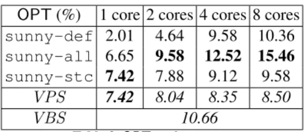
OPT (%)
1 core 2 cores 4 cores 8 cores
sunny-def
2.01
4.64
9.58
10.36
sunny-all
6.65
9.58
12.52
15.46
sunny-stc
7.42
7.88
9.12
9.58
VPS
7.42
8.04
8.35
8.50
VBS
10.66
Table 3. OPT performance.
performance monotonicity as c increases. sunny-stc reaches the peak performance with 8 cores: the VBS is outperformed 158 times (24.42% of ∆), meaning that almost one time out of four it finds a better solution than VBS .
4.2 OPT and TIME Results
The OPT performances are depicted in Table 3. This metric is challenging in our con-text: we are dealing with hard RCPSP instances for which no solver is able to prove the optimality in less than 90 seconds and the VBS can prove only 69 optimum (10.66% of ∆).
sunny-defdoes not perform well with c ≤ 2 cores, but then gradually improves by proving almost the same number of optima of VBS even without the free search variants. This means that sunny-def compensates for the lack of solvers belonging to Πall \ Πdef by properly combining the solvers of its portfolio Πdef. For c ≥ 2 the
best approach is sunny-all, which is able to outperform the VBS when using 4 or more cores. In particular, the gain with 8 cores is somewhat impressive: 4.8% optima proven more than VBS . Here the performance difference is not only due to parallelism and bounds communication, but especially to the solver selection. Indeed, the gap with sunny-stcbecomes larger as the number of cores increases. Furthermore, contrary to what happens for the OBJ metric, it is interesting to see how for c ≥ 4 the default approach sunny-def is better than sunny-stc. In other terms, adding new solvers without an adequate per-instance selection of them can be fruitful in terms of solution quality, but ineffective for what concerns the optima proven.
Figure 2 reports the number of times sunny-cp is able to outperform the VBS in terms of OPT, i.e., how many times it can prove a new optimality not provable by any other version of any given solver. The performance difference between sunny-stcand the other approaches is clear, especially for c ≥ 4. Given the low number of instances solved to optimality by the VBS , the performance of sunny-def with 4 cores (VBS outperformed 28 times) and sunny-all with 8 cores (34 times) are quite significant.
Table 4 shows the average TIME performances. Being the majority of the instances of ∆ very hard to solve, it is not surprising that the TIME values are very close to the timeout T = 900. All the tested approaches perform well, since they are very close to or better than the VBS . On average, sunny-def is able to outperform the VBS with c ≥ 4 cores. For c ∈ {1, 2, 4, 8}, the average TIME of sunny-stc is lower than the
sunny-def sunny-all sunny-stc 0 5 10 15 20 25 30 35 40
1 core 2 cores 4 cores 8 cores
N o . o f in s ta n c e s
Fig. 2. Number of times sunny-cp outperforms the VBS in terms of OPT.
TIME (sec.) 1 core 2 cores 4 cores 8 cores
sunny-def
889.33 869.42 830.71 825.55
sunny-all
858.20 838.41 823.18 797.53
sunny-stc
858.63 853.55 849.45 844.69
VPS
858.63 854.13 852.16 851.17
VBS
841.33
Table 4. TIME performance.
corresponding VPSc. This means that, even if sunny-stc never overtakes the VBS ,
the bounds communication allows to reduce the optimization time for every number of cores c. The best approach results to be sunny-all: for every c ∈ {1, 2, 4, 8} it is better than the other sunny-cp approaches and the corresponding VPSc. Moreover,
it can outperform on-average the VBS with only two cores. Its effectiveness in reducing the optimization time is also corroborated by the fact that for 41 instances (6.33% of ∆) sunny-all can prove the optimality of a solution in less than 90 seconds. 4.3 Summary
Summarizing, we can say that all the sunny-cp variants we tested can be effective on the RCPSP instances of ∆, especially when more than one core is used. The solvers parallelization is not the only key for the success of such approaches. Firstly, the use of the free search (when available) allowed us to improve the solving process. More-over, the bounds communication between the scheduled solvers enables to outperform the VBS . Furthermore, we realized that it is also important —especially for OPT and TIME metrics— to properly schedule a subset of solvers dynamically, i.e., according to the instance to be solved. A simpler static approach can be instead useful for finding good solutions as witnessed by the OBJ results. In general we might say that
sunny-allis the best approach while sunny-def is the worse one, proving that it is im-portant to use solvers able to adopt their own preferred search strategy. However, we should be careful to draw hasty conclusions. Let us show a concrete (counter)example showing the potential and the differences between the tested approaches.
Solver
mkspan
TIME (sec.)
Fixed Free Fixed Free
G12/Gurobi
N/A
—
T
T
Choco
600
597
T
T
Chuffed
593
594
T
T
G12/CPX
593
631
T
T
G12/FD
600
672
T
T
G12/LazyFD
—
—
T
T
Gecode
600
600
T
T
HaifaCSP
N/A 657
T
T
iZplus
1446 1446
T
T
Minisatid
N/A
—
T
T
OR-Tools
600
600
T
T
sunny-def
593
9.90
sunny-all
593
31.55
sunny-stc
593
T
Table 5. RCPSP Example. T is the timeout, N/A means not available, while — means no solu-tions found in T seconds.
Table 5 shows the performance of the different solvers on a RCPSP instance of ∆.8
As can bee seen, none of the single solvers of Πallcan conclude the search within
T = 900 seconds. G12/Gurobi, G12/LazyFD, and Minisatid can not find any solu-tion within the timeout. The fixed search variant here is better for Choco, Chuffed, G12/CPX, and G12/FD while for all the other solvers it is equivalent to the free one. For this instance, the VBS chooses (indifferently) one between the fixed versions of Chuffed and G12/CPX since they found the best makespan value 593, without however proving its optimality (OPT = 0 and TIME = T ).
sunny-defgreatly outperforms VBS , being able to prove the optimality of 593 in less than 10 seconds (OPT = 1 and TIME = 9.90). This is because G12/CPX finds the bound 593 in few seconds and the other scheduled solvers are restarted with such new bound. Now, Gecode can prove almost instantaneously that 593 is the opti-mal makespan, while without this help the best value it finds in half an hour of com-putation is 600. sunny-all works similarly, but more slowly. This time difference is due to the SUNNY algorithm, which computes instantaneously the solvers sched-ule with |Πdef| = 11 solvers, while with |Πall| = 19 it takes about 23 seconds for
0 5 10 15 20 25 30 35 40 45 43 27 13 9 3 2 2 1 O p ti m a P ro v e n
Fig. 3. No. of optima proven by individual solvers of sunny-all with 8 cores.
computing the schedule of the solvers. Finally, sunny-stc cannot prove the opti-mality of 593 since it schedules G12/CPX but not Gecode. Indeed, Π8,OPT contains
Chuffed (Free/Fixed), G12/CPX (Free/Fixed), G12/LazyFD (Free/Fixed), HaifaCSP, iZplus (Fixed).
The behavior depicted in Table 5 is not an isolated case. As an example, Figure 3 shows how many times a constituent solver of sunny-all proves the optimality when 8 cores are available. In total sunny-all proves the optimality of 100 instances (15.46% of ∆), 31 instances more than the VBS . Despite Chuffed Free completes the search the largest number of times (43/100), the majority of the instances are solved to optimality by other solvers. Moreover, we can not say that in this case sunny-all is enhancing Chuffed Free, since when it is executed alone it can prove the optimality of more instances (48 instances, i.e., 7.42% of ∆ as reported in Table 1). The same applies to its fixed version and G12/CPX. Conversely, sunny-all can significantly boost the individual OPT performance of non-LCG solvers like G12/Gurobi, Choco and Gecode. G12/Gurobi proves 27 optima, 8 more than its individual performance. Particularly in-teresting it is also the difference for Choco (both versions) and Gecode (fixed version) since none of such solvers is able to prove any optima when is run alone. By exploiting instead the bounds found by other solvers they can conclude the search in a not negli-gible number of times: Gecode proves 13 optima and Choco 11 optima (9 with the free version, and 2 with the fixed one).
5
Conclusions
The Resource-Constrained Project Scheduling Problem (RCPSPs) is a well-known scheduling problem applicable in many real-life scenarios. A state-of-the-art
method-ology consists in solving RCPSPs through Lazy Clause Generation (LCG) techniques, which allow to combine the strengths of SAT solving and Finite Domain propagation.
In this paper we show how it is possible to integrate Constraint Programming, Al-gorithm Selection, Multicore Computing and other search heuristics for solving hard RCPSP instances. We improve the state of the art on RCPSP solving by showing how the performance of state of the art LCG solvers can be significantly overcome by us-ing a portfolio approach. In particular, our methodology lies in the use of a portfolio of different constraint solvers for selecting and running a subset of them on multiple cores. We not only seek to predict which are the best solvers for a new, unseen RCPSP instance, but we also enable the bounds communication between the scheduled solvers. To the best of our knowledge, in the literature there are no similar approaches for solv-ing RCPSPs and variants.
Empirical evaluations conducted on hundreds of non-trivial instances show that, by exploiting different versions of the sunny-cp solver, it is possible to get parallel portfolio solvers able to outperform on-average the oracle solver that always chooses the best available solver for any given instance. Improvements are manifold in terms of both solution quality, optima proven and optimization time. We noticed in particular significant performance gains in quickly proving more optima.
We believe that this work may open the way to several extensions. Probably the most interesting ones concern the analysis of how to properly integrate and combine the (concurrent) execution of different constraint solvers. In particular, a major sci-entific challenge consists in understanding the interaction between constraint solvers. There are many open questions. Which information should be shared (e.g., only bounds, or other knowledge such as nogoods or snippets of the search tree)? When and how this information should be exchanged? When restarting a solver is useful and when is in-stead harmful?
In this work we focused on system having less cores than available solvers. Clearly, different techniques (e.g., running the same, randomized solver in parallel, search space splitting techniques) can be adopted with powerful clusters where the number of cores exceeds the portfolio size. The evaluation of portfolio approaches in such a setting is left as a future work.
Concerning the RCPSP problem, it would be interesting to compare and integrate our approach with Operations Research techniques. Moreover, it is certainly worth to evaluate and combine other search heuristics for improving the RCPSP resolution (e.g., precedence-setting searches, texture-based heuristics [7]).
From the portfolio perspective, we hope that this work can stimulate the utilization of portfolio solvers also in real-life scenarios where typically a single, dominant solver is used for solving different instances of the same problem. It would therefore be inter-esting to try to apply our approach also to other variants of RCPSP (e.g., RCPSP/max, RCPSP/max-cal, or Cyclic/RCPSP) and to other classes of problems (e.g., job shop scheduling or bin packing).
Finally, recalling that sunny-cp was used only since it was the only parallel folio solver for COPs, in the future it would be interesting to adapt and test other port-folio approaches or related techniques such as Algorithm Configuration [18–20] for the automatic tuning of solvers parameters.
Acknowledgements
We would like to thank the Optimization Research Group of NICTA (National ICT of Australia) for allowing us to use Chuffed and G12/Gurobi solvers, as well as for granting us the computational resources needed for building and testing sunny-cp.
References
1. Ram´on Alvarez-Vald´es and Jos´e Manuel Tamarit. Heuristic algorithms for resource-constrained project scheduling: A review and an empirical analysis. In Advances in Project Scheduling, Studies in Production and Engineering Economics, pages 113–134. Elsevier, 1989.
2. Roberto Amadini, Maurizio Gabbrielli, and Jacopo Mauro. SUNNY: a Lazy Portfolio Ap-proach for Constraint Solving. TPLP, 14(4-5):509–524, 2014.
3. Roberto Amadini, Maurizio Gabbrielli, and Jacopo Mauro. A multicore tool for constraint solving. In IJCAI, pages 232–238. AAAI Press, 2015.
4. Roberto Amadini, Maurizio Gabbrielli, and Jacopo Mauro. SUNNY-CP: a sequential CP portfolio solver. In SAC, pages 1861–1867. ACM, 2015.
5. S. Arlot and A. Celisse. A survey of cross-validation procedures for model selection. Statis-tics Surveys, 4:40–79, 2010.
6. Philippe Baptiste and Claude Le Pape. Constraint Propagation and Decomposition Tech-niques for Highly Disjunctive and Highly Cumulative Project Scheduling Problems. Con-straints, 5(1-2):119–139, 2000.
7. J. Christopher Beck, Andrew J. Davenport, Edward M. Sitarski, and Mark S. Fox. Texture-Based Heuristics for Scheduling Revisited. In AAAI, pages 241–248. AAAI Press / The MIT Press, 1997.
8. J. Blazewicz, J.K. Lenstra, and A.H.G.Rinnooy Kan. Scheduling subject to resource con-straints: classification and complexity. Discrete Applied Mathematics, 5(1):11 – 24, 1983. 9. Peter Brucker, Andreas Drexl, Rolf H. Mohring, Klaus Neumann, and Erwin Pesch.
Resource-constrained project scheduling: Notation, classification, models, and methods. Eu-ropean Journal of Operational Research, 112(1):3–41, 1999.
10. Jacques Carlier and Emmanuel N´eron. On linear lower bounds for the resource constrained project scheduling problem. European Journal of Operational Research, 149(2):314–324, 2003.
11. Geoffrey Chu. Chuffed source code. https://github.com/geoffchu/chuffed. 12. Geoffrey Chu, Maria Garcia de la Banda, and Peter J. Stuckey. Automatically Exploiting
Subproblem Equivalence in Constraint Programming. In CPAIOR, volume 6140 of LNCS, pages 71–86. Springer, 2010.
13. Nachum Dershowitz, Ziyad Hanna, and Alexander Nadel. A clause-based heuristic for SAT solvers. In SAT, volume 3569 of LNCS, pages 46–60. Springer, 2005.
14. Carla P. Gomes and Bart Selman. Algorithm portfolios. Artif. Intell., 126(1-2):43–62, 2001. 15. S¨onke Hartmann and Dirk Briskorn. A survey of variants and extensions of the resource-constrained project scheduling problem. European Journal of Operational Research, 207(1):1–14, 2010.
16. Willy Herroelen, Bert De Reyck, and Erik Demeulemeester. Resource-constrained project scheduling: A survey of recent developments. Computers & OR, 25(4):279–302, 1998. 17. Andrei Horbach. A Boolean satisfiability approach to the resource-constrained project
18. Frank Hutter, Holger H. Hoos, and Kevin Leyton-Brown. Sequential Model-Based Optimiza-tion for General Algorithm ConfiguraOptimiza-tion. In LION, volume 6683 of LNCS, pages 507–523. Springer, 2011.
19. Frank Hutter, Holger H. Hoos, Kevin Leyton-Brown, and Thomas St¨utzle. ParamILS: An Automatic Algorithm Configuration Framework. J. Artif. Intell. Res. (JAIR), 36:267–306, 2009.
20. Serdar Kadioglu, Yuri Malitsky, Meinolf Sellmann, and Kevin Tierney. ISAC - Instance-Specific Algorithm Configuration. In ECAI, volume 215 of Frontiers in Artificial Intelligence and Applications. IOS Press, 2010.
21. Rainer Kolisch and S¨onke Hartmann. Experimental investigation of heuristics for resource-constrained project scheduling: An update. European Journal of Operational Research, 174(1):23–37, 2006.
22. Oumar Kon´e, Christian Artigues, Pierre Lopez, and Marcel Mongeau. Event-based MILP models for resource-constrained project scheduling problems. Computers & Operations Re-search, 38(1):3–13, 2011.
23. Lars Kotthoff. Algorithm Selection for Combinatorial Search Problems: A Survey. AI Mag-azine, 35(3):48–60, 2014.
24. Stefan Kreter, Andreas Schutt, and Peter J. Stuckey. Modeling and solving project scheduling with calendars. In CP, volume 9255 of Lecture Notes in Computer Science, pages 262–278. Springer, 2015.
25. S. Lawrence. Resource Constrained Project Scheduling: An Experimental Investigation of Heuristic Scheduling Techniques (Supplement). Technical report, Graduate School of Indus-trial Administration, Carnegie Mellon University, 1984.
26. Nicholas Nethercote, Peter J. Stuckey, Ralph Becket, Sebastian Brand, Gregory J. Duck, and Guido Tack. MiniZinc: Towards a Standard CP Modelling Language. In CP, volume 4741 of LNCS, pages 529–543. Springer, 2007.
27. Wilhelmus Petronella Maria Nuijten and E. H. L. Aarts. A Computational Study of Con-straint Satisfaction for Multiple Capacitated Job Shop Scheduling. European Journal of Operational Research, 90(2):269–284, 1996.
28. Olga Ohrimenko, Peter J Stuckey, and Michael Codish. Propagation via lazy clause genera-tion. Constraints, 14(3):357–391, 2009.
29. John R. Rice. The Algorithm Selection Problem. Advances in Computers, 15:65–118, 1976. 30. F. Rossi, P. van Beek, and T. Walsh, editors. Handbook of Constraint Programming. Elsevier,
2006.
31. Andreas Schutt, Thibaut Feydy, Peter J. Stuckey, and Mark Wallace. Why cumulative de-composition is not as bad as it sounds. In CP, volume 5732 of Lecture Notes in Computer Science, pages 746–761. Springer, 2009.
32. Andreas Schutt, Thibaut Feydy, Peter J. Stuckey, and Mark G. Wallace. Explaining the cumulative propagator. Constraints, 16(3):250–282, 2011.
33. Andreas Schutt, Thibaut Feydy, Peter J. Stuckey, and Mark G. Wallace. Solving RCPSP/max by lazy clause generation. J. Scheduling, 16(3):273–289, 2013.
34. Peter J. Stuckey, Ralph Becket, and Julien Fischer. Philosophy of the MiniZinc challenge. Constraints, 15(3):307–316, 2010.
35. Peter J. Stuckey, Thibaut Feydy, Andreas Schutt, Guido Tack, and Julien Fischer. The miniz-inc challenge 2008-2013. AI Magazine, 35(2):55–60, 2014.