HAL Id: hal-03001840
https://hal.archives-ouvertes.fr/hal-03001840
Preprint submitted on 12 Nov 2020HAL is a multi-disciplinary open access
archive for the deposit and dissemination of sci-entific research documents, whether they are pub-lished or not. The documents may come from teaching and research institutions in France or abroad, or from public or private research centers.
L’archive ouverte pluridisciplinaire HAL, est destinée au dépôt et à la diffusion de documents scientifiques de niveau recherche, publiés ou non, émanant des établissements d’enseignement et de recherche français ou étrangers, des laboratoires publics ou privés.
How far can we go? Determining the optimal loan size
in progressive lending
Nahla Dhib, Arvind Ashta
To cite this version:
Nahla Dhib, Arvind Ashta. How far can we go? Determining the optimal loan size in progressive lending. 2020. �hal-03001840�
How far can we go? Determining the optimal loan size in progressive lending
Dr Nahla Dhib
LJAD laboratory, Mathematical departure Campus Valrose, Cote d'Azur University, Nice France
Dr. Arvind Ashta
CEREN EA 7477, Burgundy School of Business, Université Bourgogne Franche-Comté, Dijon, France
Abstract
The microcredit literature indicates that progressive lending should reduce default rates but that it may lead to over-indebtedness. In this study, we show that progressive lending may be safe over a range of loan sizes, beyond which a rational borrower would indulge in a strategic default. This range of loan sizes may be dependent on borrower characteristics (risk -taking, self-confidence, productivity, interest rates, subsistence needs) as well as the Microfinance Institution’s strategy. Many crowdfunding sites are using artificial intelligence to assess borrower risk through social ratings. We are arguing that production functions of the borrowers also need to be added.
1. Introduction
The World Bank reports that only 69% of adults have a bank account (Demirgüç-Kunt et al. 2018). Their report indicates that only 47% have taken a loan, and this is lower at 44% in developing countries. Indeed, one of the most important growth objectives of banks is lending to the poor and the World Bank is devoting considerable energy to gather data and report on the leve l of financial inclusion. It is important in this objective that appropriate loans are given to people depending on their specific characteristics and needs. For this, supply side constraints on providing customized loans may be overcome by using artificial intelligence wisely (Makridakis 2017; Pansera, Ehlers, and Kerschner 2019).
In the past, bankers hesitated to lend directly to the poor owing to 1) information asymmetries that increase the risk; 2) lack of complementary social and human capital; and 3) small loan sizes that increase the cost of providing small loans, and microfinance institutions (MFIs) have come in to fill this market gap (Armendàriz and Morduch 2010). On the first issue, there is a large literature on the reasons for market failure, credit rationing or over-lending, owing to asymmetric information, focusing on adverse selection and moral hazard (Akerlof 1970; Stiglitz and Weiss 1981; de Meza and Webb 2000). In lending, the adverse selection problem of the lender is not being able to distinguish safe from risky borrowers b efore the loan is given; while the moral hazard increases if interest rates are high, thus leading to a backward bending supply curve. Over the last several decades, bankers have developed credit scoring tools that help
bankers make decision on borrower risk, but these scores are influenced by credit histories (Bumacov, Ashta, and Singh 2017).
Microcredit is often considered a leading social innovation because it involves giving loans to poor people, thus giving them a chance to finance their venture and escape poverty, despite a lack of cr edit history (Ashta et al. 2013; Armendàriz and Morduch 2010). Microfinance Institutions were able to give loans with low default rates because they used a number of schemes to overcome the low transaction size and asymmetric problems of lending to the poor: for example, group lending (Besley and Coate 1995; Ghatak 1999; Guttman 2008), lending only to women (especially in South Asia), frequency of loan repayments, and progressive lending (Egli 2004; Singh and Padhi 2017). As a result, many MFIs had loan repayment rates of above 99%. As borrowers moved from group lending to individual lending (Dowla and Barua 2006), the use of credit scoring started being adopted by MFIs and this has indeed made the credit officers more productive, thus increasing their outreach and the financial inclusion of the poor (Bumacov, Ashta, and Singh 2014).
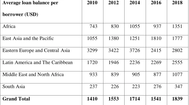
The second problem of microfinance was the small transaction size as can be seen in Table 1. The average loan size is $1839 in 2018, after filtering out the database of the Microfinance Information Exchange (MIX) for loans greater than $30000. However, the median loan size is much lower: the global median is $684 for 2018. The low transaction size, meant that operating and transac tion costs were high and consequentially interest rates were high (Rosenberg, Gonzalez, and Narain 2009; Shankar 2007). One way to lower costs is to standardize loan products and operational procedures (Khan and Ashta 2012; Akula 2010). Considerable effort to reduce these costs and improve performance is also being made through advanced technologies (Li, Hermes, and Meesters 2019; Soltane Bassem 2014), notably crowdfunding to reduce financing costs (Attuel-Mendes 2014; Allison et al. 2015; Assadi 2016),
information systems to reduce information processing costs (Iyengar, Quadri, and Singh 2010), and mobile banking to reduce delivery costs (Morawczynski 2011; Shrivastava 2010). The most promising of these,
mobile payments, has received global attention since many the unbanked in Africa and Asia have mobile phones. However, as mobile loans have gone up, repayment rates have fallen. The difficulty of the lenders is that they cannot anticipate the behaviour of the borrower if there are no credit histories. They are therefore turning to social credit scoring using the big data available on telephone and internet networks to analyse the personality of the potential borrower.
Insert Table 1 about here
The use of social data for credit scoring in the developing world was probably pioneered by Lenddo, a company that operated in Philippines and Columbia and has since expanded (Hardeman 2012). These credit scoring algorithms are improving thanks the increasing use of artificial intelligence and machine learning. Many startups all over the world are bein g financed by venture capitalists including the International Finance Committee (IFC), the private investing arm of the World Bank group. For example, In Africa, Credit Suisse is trying to capture similar data from mobile telephones, using biometrics and facial recognition for identity checks as well as behavioural characteristics captured on their telephone including calling histories and financial transactions (Crosman 2017). With the development of artificial intelligence and machine learning, and with the increasing use of mobile and internet banking, such customization of financial services to borrower’s
estimated needs is not only possible but will be essential to competitivity of financial service providers (WEF 2019).
Our economic intuition that motivates this study is that these algorithms will improve if, in addition to the borrower’s social profile, their capacity to produce revenue greater than the loan repayment is also considered. This means that the borrower characteristics should include production functions appropriate to the size and sector of the borrower’s business. These production functions themselves can be estimated dynamically based on machine learning.
To resume our study in a nutshell, lenders want to increase financial inclusion and make profits. For this, they want to give more and bigger loans and yet ensure that t he borrower reimburses so that they make a profit. Our study shows that there is a range of loan sizes below which there is credit rationing and above which the borrower would make a strategic default, and this depends on the borrower
characteristics, their production function as well as the strategy of the financial institution.
The next section provides a brief literature review of the borrower characteristics that may influence this progressive lending. We then introduce a simple model to understand the equilibrium position using Markovian Chains. Once the basics of our model is clear, we introduce how their
perceived production function may limit the possibilities of their graduation to future stages, depending on their perceptions of optimal loan size and how the behaviour of borrowers depends on their perception of the lender’s objective of financial inclusion.
2. Literature review
The economics of microfinance considers that the poor always pay back because they fear that nobody will give them a second chance if they do not repay (Yunus 2003). Indeed, many microfinance authors indicate that part of the dynamic incentives provided by microfinance institutions (MFIs) is new loans, and
even bigger loans, to successful entrepreneurs who pay back and threats to stop lending to those who do not (Armendàriz and Morduch 2010; Egli 2004; Shapiro 2015). Yet, entrepreneurship evidence indicates that half the small business enterprises close within three to five years (INSEE 2012), indicating that micro-entrepreneurs who grow may be the exception rather than the rule and that dynamic incentives have a bias towards those who are confident of success.
At the same time, if one poor person does not pay back, the MFI knows that there is a risk of contagion and no one would pay back (Bond and Rai 2009). Therefore, MFIs are vigilant on their solvency issues (Schulte and Winkler 2019). Since it is too expensive to use legal enforcement for such small loan sizes, the MFI must either coerce borrowers to pay back or it must find a valid reason for rescheduling the loan such as attributing the failure of the entrepreneur to an external shock (earthquakes, floods, typhoon). The MFI is therefore interested, financially, in increasing the loan size for successful entrepreneurs, as well as refinancing those failed micro- entrepreneurs who have a chance to be
successful later (Dowla and Barua 2006), which we call a second chance. It may also be interested in a social objective: to graduate people to financial inclusion where they may get even larger loans at market conditions. Indeed, some researchers consider that with progressive lending, it is normal that average loan sizes should increase.
Yet, there may be a limit to the loan sizes that microfinance borrowers take because it may be possible to earn less with bigger loans if the production function flattens with increasing capital, assuming a sole entrepreneur (no employee). Although there is evidence that this is the case (Mahmood, Hussain, and Z. Matlay 2014), there is still a need to explain the existence of this optimal loan size theoretically.
The optimal loan size may differ for heterogeneous people and segments of people. For example, Agier and Szafarz (2013)) find that there may be glass ceilings from the lender’s side and women are provided smaller loans, and they therefore make smaller profits. However, it is also possible that women may consider that the optimal loan size is smaller and may request smaller loans and make smaller profits.
They may, therefore, be less inclined to graduate to large loans and towards complete financial inclusion till their self-confidence and skills are improved.
We know that MFIs lend more to a village that it close to market or if there is high agricultural productivity (Mallick and Nabin 2018). This may be because MFIs seek to give loans where the repayment rates are expected to be higher. In other words, MFIs intuitively look at the production function of the borrower. This is similar to banks which also give more loans in expansionary business cycles when expected production is more important (Hyun and Uddin 2016). Therefore, in this paper we incorporate the importance of the production function into our model.
This paper is prescient of the importance of this question of financial inclusion in the years to come. Indeed, as microfinance markets grow and saturate, loan sizes are increasing because MFIs try to offer bigger incentives to attract clients. MFIs may offer different kinds of loans because clients have different preferences: risk averse borrowers are less willing to take up individual loans and less selfish borrowers may prefer joint liability loans (Baulia 2019). Therefore, customization is essential for growth.
Along with growth of MFIs, default rates are increasing since screening levels are falling and borrowers may borrow from multiple lenders (Mallick and Nabin 2018). As borrowers resort to multiple- borrowing, a recognized problem in growing and saturated markets, they are
effectively increasing their probability of a second chance. Although credit bureaus may limit multiple borrowings, even multiplying borrowing from one MFI to two, increases the probability of a second chance. Both these factors increase the effect of default (size and probability).
In this study, we contend that MFIs could look at the production function of the MFI and use it to decide the point at which progressive loans should stop till the production process becomes more productive.
Tedeschi (2006) shows that for progressive lending to work, the borrower’s profitability must be high, lending costs must be low, the risky group of borrowers cannot be too risky, and the average probability of default must be sufficiently low. However, she did not look at the range of loan sizes for which progressive lending might work. Developing her perspective, we offer further insights to borrower needs and the decision process behind borrower behaviour.
Our study helps in understanding the dynamics of the interaction between success and failure probabilities perceived by microfinance borrowers as well as their perceptions of the possibilities of a second chance (rescheduling), on the one hand, and the objectives of the MFIs to offer them loans, and then graduate them from microloans to bigger loans and, eventually, to financial inclusion, on the other hand.
3. Research Methodology
The research question we have asked is not why people default but how to determine at what point of a progressive loan cycle a person would default so that the lender can stop lending to an otherwise good customer.
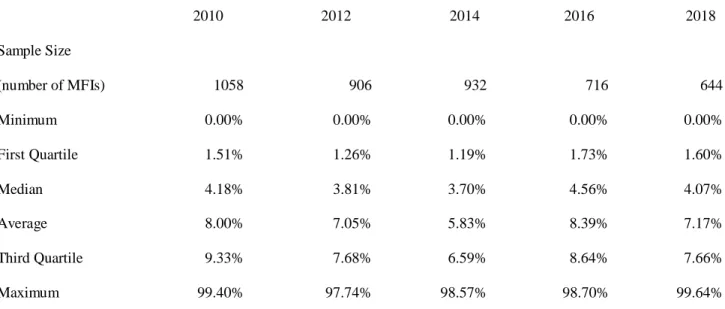
We confirmed that these are important questions based on preliminary interviews with executives from four MFIs. Since one of these respondents indicated that they were never concerned by defaults, we checked the MIX data for the most used indicator of risk in microfinance: the PAR-30, that gives the portfolio that is at risk if payments are delayed by more than 30 days, as a
percentage of the total loan portfolio. We can see from the following table 2 that indeed a quarter of MFIs may not be very concerned by the default question because they may have good control systems; but the median PAR-30 is 4.07% in 2018. The average is pulled up by extreme values and is close to the third quartile. The data shows that half of the MFIs are living with high credit risk and that a quarter may be seriously facing this problem.
To answer our specific research question, the methodology we use is that of a thought experiment. Thought experiments have been used in diverse fields: philosophy (Rawls 1971), ethics (Caste 1992; Wempe 2008) economics (Margolis 1982; Kessler and Masson 1989; Lucas 2003), political economy (Mankiw 2013) and business (Elkington, Emerson, and Beloe 2006). Our thought experiment starts, as a first step, with understanding why different people chose to default which helps in understanding why people may default in different situations. We then add, as a second step, the simple economic production function to show that the same person could default as their firm becomes bigger, even if their other characteristics do not change.
For the first step, there are many studies and textbook that explain why people default. We provide an alternative perspective to these studies using Markovian chains. A large number of high level journals in management (Gershkov, Moldovanu, and Strack 2018; Ibrahim, Armony, and Bassamboo 2017; Zhang 2009) have used Markovian Decision processes highlighting their importance in furthering understanding. From our study, we show that Markovian models provide insights which could be specific to the individual decision making for taking bigger loans or for defaulting.
Markovian chains are simplified systems that are used to explain different stages in a process and the possible transition from one stage to another, using probabilities that are fixed and known. They are extensively used in economics and social sciences, but most researc hers use finite number of possible states. We use the stochastic process to explain the dynamic of borrower's rational behaviour and the lender's decision which affects the actions of beneficiary. If we imagine a set of poor beneficiaries of successive loans, the use of Markovian chain lets us estimate the probability and proportion of borrowers reaching inclusion.
In an information asymmetric environment, a MFI may use a pooling model to separate the quality of borrowers (bad or good) through group lending ((Banerjee and Cadot 1996; Van Tassel 1999). Of course, there may be different approaches provided by MFI' to separate the type of lending under specific assumptions. For example Ghosh and Van Tassel (2013), used a separating model to show that encouraged donors to invest in microfinance as this may lead to poverty reduction and ensure a perfect equilibrium in a market where the lender compensates the higher interest rate by decreasing his funding cost. In our case, we used. Markov chain in an individual loan setting. We do not use pooling, except if individual borrowers can be grouped by similar characteristics through cluster analysis. We analyse the sequence of successive loans during transition from a state to another, potentially leading to inclusion.
For the second step, we add a simple Cobb Douglas production function. This simple function is even simpler in microfinance because most micro-entrepreneurs work alone of have a part-time helper. As a result, the labour component of the Cobb-Douglas function can be assumed to be 1 and the production function simplifies to be dependent largely on the amount of capital invested, the productivity of the capital and that of labour and capital working together. Assuming further that poor people have some small fixed savings, the production would then depend upon the microcredit that the person can avail.
While the economics of each step is simple, the novelty of combining them leads to determining, for each individual borrower, at what point a rational borrower may prefer to strategically default. Most of the simplifying assumptions that we have made can be relaxed by using computers and machine learning, in the near future, can improve the parameters that we may have taken as fixed to describe this thought experiment.
4. Modeling the strategies of borrowers
In this section, we build our basic model using Markov chains. We consider a
beneficiary who takes a microcredit to create a small business and produces an income. If she succeeds in the small business, she receives successive larger loans. We assume that at the first state M, she invests and if she succeeds, she gets to the second state B with a bigger loan. At each stage, the behaviour of borrower is influenced by the financial capital and human capital as well as future expectations. These future expectations are based on a production function which tapers off. Costs increase linearly. Therefore, profit expectations are parabolic, init ially increasing and later decreasing. To take care of this, we need three stages rather than two: the first two stages could be on the increasing phase and the third could be on the decreasing phase. Therefore, we suppose that if she succeeds at B, she gets to inclusion state I. At any time, if she loses, she returns to exclusion state E. We define a trajectory ω = (M, B, I, E) where M is initial micro loan size, B is big loan size, I is inclusion, E is exclusion.
Additionally, we assume that the lender has a financial and a social objective and seeks to maximize the proportion of inclusion (π). This means that the lender would like the borrower to improve her financial state and succeed in her activity. This would also allow the borrower to repay the loan, ensuring the profit of the lender. The borrower’s success depends on her ability to manage her small business and she identifies her strategy during the trajectory taking in account the success probability of the small activity.
We suppose that the economic activity of the borrower follows a trajectory ω with known transition probabilities from each state (αM, αB , αI , γE ). We further consider that the
dynamics of borrower behaviour depends on these success probabilities that can be captured by a Markov chain. These alphas capture not only the capacity of the borrowers but also their preferences. For example, some borrowers may prefer to remain unemployed unless they find an extremely high return project letting them become millionaires. Others may be willing to work for a small profit to avoid a situation of idleness. This may partly depend on their respective initial wealth. Similarly, the alphas also capture their desire to make a strategic default or not to do so. We assume that 1 − γ captures the
expectation of the borrower to get a second chance if she loses (and defaults). This expectation may be determined with respect to stationary strategy of the lender in terms of providing refinance, the number of alternative lenders, and if the lenders have information on the previous defaults of a borrower through credit bureaus. This implies that decisions of the borrower are influenced by perceptions of lender’s actions.
Any borrower’s actions are determined by success probability pi of a process of Markov Chain (Xt), defined at a state (i) of a set (ω) with πi > 0,), πi = 1. This stochastic process is illustrated in Figure 1.
Insert figure 1 about here
Drawing all probabilities in Figure 1, we define the transition matrix (P) where the rows indicate the current state and the columns indicate the transition state, as shown below (equation 1).
Referring to the property of Markov chain to solve a stationary distribution, we define a vector of lender’s objectives π whereby he aims to bring his borrower to financial inclusion through a trajectory ω = (M , B, I, E). This vector summarizes the proportion of borrowers who move from a stage to the next one. For example, the lender may have an objective of providing micro loans to a fraction of the excluded people. Later, he may graduate a fraction of this first fraction of people to a bigger loan. Then, he may graduate another fraction of these second fraction of people to inclusion. Finally, he may try to keep on servicing a fraction of the included people by matching the offer of banks.
Therefore, the borrower is facing an MFI which has its own objective for borrowers in different states (M , B, I and E). For example, it may decide that it would like 20% of the excluded to be given loans (πM ), 20% of those who get microloans to be graduated to big loans (πB ), 20% of the big loan recipients to get even larger financial inclusion loans at commercial rates (πI ). Finally, it may decide that 20% of those who default would be given a second chance (πE ). These objectives of the lender are captured in the vector,
V = (πM , πB , πI , πE ) (2)
Equilibrium distribution will result when we multiply the borrower’s transition matrix P by the vector of the lender’s objectives V.
To optimize the borrower’s inclusion position, we maximize the previous expression (3) to provide an equilibrium state, which gives,
This equilibrium stage will be achieved only for 1 − αM > 1 − αB or π*E=0
We can see from equation (4) that an optimal strategy for inclusion is dependent on the risk of success or failure in each State as well as the probability 1 − γ capturing the expectation by the borrower of the proportion of people to whom the lender will provide a second chance and πE is the proportion of excluded people to whom the MFI would like to offer loans. This objective may depend on the funding availability of the MFIs as well as its perception of the human and physical capital and chance of success of borrowers in that area. These do not necessarily exclude those who have lost once since the MFI will look at the whole market of the excluded.
In each case, we keep four States where a borrower can either advance one stage in a period or return to exclusion.
I. Dynamics of Interaction between Borrower Strategies and lender Objectives
Assuming all probabilities of transition are known, we could have an optimum solution which results from the interaction of the strategy of the borrower and the objective of the lender to lead the borrower to financial inclusion. What would this be? What do we learn from the stochastic process? Each borrower is different, and we could have thousands of cases which could be regrouped. Here, we illustrate with five cases, with different probabilities of transition from one stage to the next, reflecting that borrowers are heterogeneous in capabilities and preferences. For example, in case 1 we assume equal probabilities of 0.25 of success but with larger probability of failure, but most failures lead to an
expectation of a second chance (with probability of 0.75); in case 2 we increase the probability of success with large loans and maintain the high probability of second chance; in case 3, we maintain the low probability of success of case one but reduce the probability of second chance to 0.2; in case 4, we
increase the probability of success further and take an intermediate perception of the probability of second chance. The Table 3 clarifies the differences between these 4 simple cases. Finally, in Case 5, we introduce more complexity where the borrower can not only succeed to the next stage but could also remain in the same stage or even go back one stage, with an intermediate probability of a second chance of 0.4.
Insert Table 3 about here
Case 1: In this situation, we can suppose that the lender is financing risky activities since the success probability is low (αM = 0.25). This means that it may lead to a difficult situation where bad debts are anticipated (αI = 0.25). Its detrimental for the MFI to lend to borrowers in such situations since it is unlikely to lead to financial inclusion. Therefore, the lender needs to provide a second chance, and this is captured by the high probability of 0.75 (1 − γE ) to try to bring the borrower back towards inclusion. This provides borrowers a situation where they can make a strategic default, knowing that they may get a second chance. In fact, they carry on their risky investments with the same probability of success (αB = 0.25).
However, the second chance means that loans are being given to refinance by deferring the loan repayment. This is usually the case where the default amount is a small part of the microloan. Otherwise, if the default is a large part of the loan, it means that if the business i s to continue, the total size of the loan increases and the total risk increases for refinanced
borrowers because they have not yet repaid the first series of loans and the fact of taking a second microcredit makes the borrower more vulnerable and increases her debts. To make it simple, we assume that the borrower will start a new business and start the markovian cycle with a loan (M) either from this MFI or, more probably, from another MFI who does not have access to the credit history of default.
We note that different iterations with different values for an initial starting vector V for the lender will change the final V. However, the proportions as a function of πE remain stable at those indicated in V ∗ below. These proportions are dependent purely on the parameters of the transition matrix (1). We deduce that the best cycle for this combination of borrower strategy and lender objective is cycle 3 for Microloans, Inclusion and Exclusion, while bigger loans perform better in cycle 4. This means that success in large loans after success in
microloans is difficult to achieve and, therefore, the chance of exclusion goes up and the chance of inclusion reduces. This could explain the initial optimism of microfinance. For example, Servet (2015) and Tedeschi (2008) show that successive loans can help some and increase the vulnerability for others, but they do not mention why.
We also deduce that the result of the lender at the end of the period shows the fraction of borrowers who achieve the inclusion state by trajectory of (M,B,I,E) is less than the part of exclusion. This consequence creates a disappointing result for the lender who seeks to
maximize inclusion but finds that a very small part of the excluded population attains this state.
We reach an interesting conclusion which can help the lender to optimal decisions. If the lender selects risky borrowers, the lender should assure the accompanying and the
controlling of borrowers to improve her business and increase the profit probability (αB > αM ), but this increases the costs for the lender. This strategy of accompaniment and coaching reduces the vulnerability of the borrower by improving her skills, thus leading to graduating to a larger loan size with less chance of failure. We examine this in case 2. Alternatively, to improve inclusion, the lender could also reduce the perception of the possibility of second chance of a borrower by increasing his γE. This would then entail a decisive step against strategic default
and facilitate the selection of less risky activities by the borrower. We examine this later in case 3.
Case 2: We now study a second borrower with better capabilities for running a small business (B) and otherwise similar preferences to case 1 (see Table 3 for details). During this trajectory, compared to the borrower in case 1, the situation of borrower is the same in the first period (M to B), but is less risky in the second stage because of economies of scale or owing to better management due to better skills (B to I) and therefore we assume that the borrower increases her success probability αB > αM . However, when the business becomes too big, she is unable to manage it any better than the first case. The borrower assumes that there is the same high chance to be given a second loan of size M by the lender. Again, we find that she prefers to return to E than to carry on to I.
We find that the part of inclusion after 4 states is better for the second borrower than the first case because of the higher (αB > αM). However, the lender still finds that the stable
situation is below the initial objective of inclusion. The borrower carries on her micro-business, but it never leads to inclusion since she anticipates a low probability to succeed if this business becomes too large. We can deduce that lender loses the chance for creating inclusion.
The lender may, therefore, require a strategy of providing skill training to the borrower to improve the success probability in State I. This would then promote the lender’s objective of financial inclusion (we will see this in Case 4). However, we first see, in Case 3, the effects of a strategy of the lender to decrease the borrower’s perception of the probability of second chance to return to the state M after losing in States M, B or I.
Case 3 : We examine what happens if the MFI reduced the borrower’s perception of a second chance (see Table 3). We find, therefore, that if the perception of a second chance is low, the borrower would have an even lower preference to continue to the inclusive state, compared to the first case. Overall, it is still not very encouraging for the lender since a lot of people are excluded and they will have high bad-debts of the people who fail along the way. However, it allows them to rotate the borrowers and have new borrowers (in the following stage) who may succeed better.
Comparing case 2 to case 3, we can say that it is better for the MFI to select more competent borrowers or less risky activities than to reduce the perception of a second chance. This would then make a compelling case for using credit scoring tools.
Case 4: It is clear that if we took a combination of case 2 and case 3, the inclusion rate may go up or down. However, if we want inclusion to go up substantially, we need a bigger change in
assumptions and select borrowers who are more competent or activities that are less risky and keep some intermediate chance of refinancing (see table 3).
Since the probability of success is higher than the first three cases, the borrower represents a good client for lenders who select less risky activities and more competent micro-entrepreneurs. Assuming that borrowers finance their small business by successive loans, we calculate the part of inclusion. We find from this case that it is possible to bring more than half of all potential borrowers into inclusion. However, this may require compromises: for example, the MFI may need to discriminate against the most vulnerable persons who may be less competent and riskier. As a result, the MFI may have to adopt a top-down approach in the sense of first including the not-so-poor and then gradually moving to the very poor.
Case 5: Having understood the simple Markovian models with either/or possibilities in each case, we now introduce a slightly more realistic model where the borrower can progress, remain in the same situation, or regress. This means, for example, that one can progress (from M to B) or that one can remain still in the same state (M to M), or one can return to previous states (B to M). We suppose that α is the probability of the borrower to remain in the same state during her trajectory ω = (M , B, I, E), β is the probability when the borrower succeeds to get to the next state and λ is the probability of the borrower returning to a previous state. However, in each state, the borrower has a risk of failure and falling back to exclusion represented by (1 − α − β). For this case, we assume that the lender proposes an intermediate perception of probability of second chance (1 − γ). Based on these assumptions, the trajectory of the micro entrepreneur is illustrated by the figure 2:
Insert Figure 2 about here
As in the preceding cases, the lender aims to maximize inclusion. Referring to the property of Markov chains (see equation (2 and 3), the following expression describes the stationary distribution,
We find that with such dynamic assumptions, and a good interaction between borrower strategies and lender objectives, we can have a reasonable inclusion rate.
Based on the above, we can see that the MFI and the borrowers can play on the different success rates and perceptions, as well as on the final inclusion objectives of the MFI. The use of Markovian model lets us understand the impact of each of these in the different states and the MFI can play on these to select its borrowers as well as help them develop appropriate skills for greater success. This explains why many MFIs and crowd lending sites are building complicated credit scoring models to incorporate borrower
characteristics.
However, we can go one step further, and see how Markov chains help us learn more about the fragility of customers falling from inclusion to exclusion or rising from exclusion to inclusion by introducing an additional element: the expected cash flow produced from small business financed by small loans.
Insert Figure 3 about here
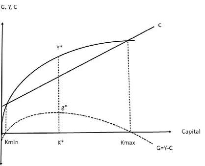
II. Introducing Expected cash flows into the Markov Chain analysis We introduce a rationality constraint incorporating that success means earning an income from the business. We assume that cash flows and income are the same since it is only working capital that is usually financed in thAis setting. It is only if borrowers cover all charges in each state that they can grow in the
small business from M to B and from B to I by increasing the size of loan. In terms of our diagram (figure 3), we suppose that a borrower can provide her irreducible consumption at a non-zero intercept but that as income increases owing to loans, she pays more interest to finance her small business. Therefore, the consumption curve is upward sloping. The borrower produces her net income (gross of interest expense) according to the concave curve. We are effectively assuming that borrowers have no other income.
The borrower aims to maximize her earnings (g = Y − C) after taking care of her reimbursement and her consumption needs (C). The income (Y) is assumed to follow a Cobb-Douglas function, and we accordingly suppose that the borrower produces an income Y (K, L) = Kθ ∗ L1−θ , where K is capital and L is Labour. In the case of our micro-entrepreneurs (L = 1) since they do not employ anyone else, they each produce a total income Y (K) = η ∗ Kθ ) where η > 0 includes the human capital added by the coaching and training of lender. The borrower expects financial charges (K ∗ r) which represents the reimbursement of loan and the consumption needs (C = K ∗ (1 + r) + c). Note that,
g(K, r) = η ∗ Kθ − (K ∗ (1 + r) + c) (12)
Combining this constraint with our earlier discussion on Markov chains in part 1, we can say that the continuation or progress of a borrower in states M, B or I assume that she expects a positive result g in each state. Otherwise, she would default and go to E. Thus, the alphas of success in M, B and I are a function of g being positive, which itself depends on Y and C, where Y depends on the productivity of capital and the coaching provided by the lender.
To calculate the optimum contract on this scenario, we suppose a function f for any borrower (x) who has a trajectory of states (M , B, I, E),
where the lender offers his borrower a lower interest rate (r− < r) to stay with the MFI, rather than going to a bank, in the inclusion state.
Using our Markov chains of figure 1, we calculate the expected net cash flow (Z) on transition from actual state to next one by the following equation,
Z(xt, xt+1) = E(f (xt+1)|xt) (14)
What can we then say about the optimal loan size as a percentage of Z and how does the set of probabilities of success influence it? To answer this question, we discuss the optimal cash flow expected (Z) on transition from one state to another which leads to financial inclusion depending to the size of
microcredit.
Z(xt, xt+1) = αxt ∗ g(xt, xt+1)(K, r) (15)
To link the two parts of our discussion, we illustrate in the following cases how this ties together. For each case, we take three scenarios with loan sizes of 1000, 2000 and 3000 corresponding to states M, B and I. Although meant to be purely illustrative, these are reasonable in view of the world average loan size as can be seen from Table 1: the microloan is smaller than the world average, the big loan is slightly bigger than the world average and the borrower included has a much larger loan size. We assume the expected cash flows for the business model are the same for any business, borrowers are heterogeneous and their success probabilities (α) are different, as stated in equation
We develop the five cases of part IV and for this we take their respective αs and the γ. Figures 4 to 8 show the expected profits for the five cases in each of the four states (M,B, I E) as determined by the assumed production function.
Insert Figures 4 to 7 about here
* Case 1: At first glance, expected profits are increasing in each state and we would expect the rational borrower to be incentivized by bigger loans. However, if the borrower has a high expectation of a second chance, we note that in exclusion she has an expectation of Z(E, M ) = 49.47. Therefore, rather than go from M to B, she would prefer to default and go to E. Our first insight is that there are situations where only the borrowers who are straight away given loans of size B that feel incentivized to want bigger loans of size I. Therefore, we can conclude that for this kind of borrower, we may need to give bigger loans from the beginning. Alternatively, in opposition to part I, the lender needs to reduce the perception of the second chance of the borrower. This additional insight would not have materialized if we had not introduced the production function.
*Case 2: This kind of borrower has higher expectations in the intermediate Big loan than in the biggest I size loan or in the exclusion state. So, for this borrower the best would be to stay in the B state rather than opt out to go to exclusion or try to progress to inclusion. However, in the Markov chain we defined that she cannot stay in the same state. The MFI will try to push her to I, and she prefers this to exclusion where she expects only Z(E, M ) = 49.47. Our second insight is that there are situations where full inclusion may not be the best outcome for poor borrowers faced with such probabilities of success. Alternatively, as discussed in the previous part, the lender must provide training so that the borrower increases her perception of success in the last state and wants to go towards financial inclusion.
*case 3: αM = 0.25 < αB = 0.5 > αI = 0.25: As shown in Figure 6, if the borrower carries on her small business on trajectory (M to B to I), she expects earning (Z(M , B) = 16.49 < Z(B, I ) =
47.84 < Z(I, I ) = 63.69. Therefore, normally she is incentivized to continue towards financial inclusion. Moreover, since we have drastically reduced her perception of second change to 0.2, we find that her expectation in exclusion is very low Z(E, M ) = 13.19 . This confirms our insight that the threat of stopping lending is a great incentive to continue towards financial inclusion, if the borrower perceives that the threat is realistic.
*case 4: Although the numbers differ, we see that the results are similar to those of case 3. This kind of borrower is more confident and has higher expectations of success and would also not be tempted to opt out.
*case 5: As mentioned earlier, the first four cases provide simple insights that can be gained by using the Markov chain, while the fifth case is more realistic and the new Markov Chain
illustration (figure8) provides a very rich understanding. The total expected probabilities seem to give a simple result, comparable to cases 3 and 4. However, the devil is in the detail because no one has the possibility to do all the different things: they must choose between progressing, staying in the same state, regressing or defaulting. As shown in figure 8, the person who decides to progress seems to be most rational since all these probabilities are increasing Z(M , B) < Z(B, I ) < Z(I, I )) and more than the expectations with a second chance Z(E, M ). However, what happens to someone who fails in her quest for progress? We find Z(M , M ) < Z(B, B)) if staying at same state. This means that those who fail in the M stage, would be tempted to default (Z( M , M ) < (E, M )), while those who are in the B Stage would be happy to stay in that state (Z(B, B) > Z(E, M )). However, if the loss is too high, then the borrower needs to come back and the expectations reduce (Z(B, M ) < Z(I, B)) if returning to previous state. Here, we find that the borrower would rather default than be given a smaller loan since
these expectations are lower than Z(E, M). Thus, the insight we get from all this is that once such a person is financially included, it is difficult for her to borrow less. She would be happier to default than get smaller loans.
Insert Figure 8 about here
Depending on the risk preferences of the borrower, her expected incomes, the perception of possibility of a second chance, and her ability to manage a small business at different scales, she may either continue her business or exercise a default option.
III. The impact of optimal loan size on financial inclusion objectives This decision to continue or to default may depend on the optimal loan size. If the borrower is below the optimal loan size, she would try to stay along the trajectory of financial inclusion. However, if she perceives that taking a bigger loan is beyond the optimal loan size, she may not proceed further, and may even default. Therefore, it is important for the lender to understand what each borrower considers her optimal loan size, depending on her productivity and in each stage (M,B,I,E).
The lender can then decide his loan offerings according to the optimal loan size for each borrower type, which in turn depends on their human capital and their level of consumption. As illustrated in Figure 9, continuing from equation (23), in each state, g = Y − C needs to be positive. Therefore, there is a
minimum capital size, Kmin and a maximum capital size Kmax, which determine the range of viable alternatives. However, we can see that there is an optimal capital size which maximizes the net gain (g), i.e., it maximizes the difference between Operating Income (Y) and Consumption (C). We can see that the more the size of the loan increases, the borrower anticipates more charges
(KB > KM => r ∗ KB > r ∗ KM ) during the following transition state. In fact, she should produce a net income g(KB , r) > g(KM , r). This will be true if the production function Y is still greater than the consumption function C.
Insert figure 9 about here
We can deduce the optimal loan size k∗ for any productivity fraction of θ provided by the borrower from the equation 23.
K∗ = (η ∗ θ/r)1/(1−θ) (16)
The additional insight that we can get from this is that since this gain (g) reduces after k∗, the borrower will not want a loan bigger than K∗ . Therefore, if the financial inclusion loan size (I) is more than K*, the borrower may prefer to stay at a lower level (M or B) or even default (E). Thus, the lender needs to either ensure that the loan size for financial inclusion (I) is smaller than the borrower’s k∗ or that he finds way to increase the borrower’s k∗ by either lowering interest rates or by suggesting more productive business lines to the micro entrepreneur, thus increasing the productivity of capital (θ) or by increasing the productivity of human capital through training (η).
7. Discussion, Practical implications, and Concluding Remarks
Part 3 of this study has shown that Markovian models are useful to understand the interaction between borrower strategies and lender objectives by clarifying that there are diverse kinds of borrowers
and lender strategies need to adapt to this heterogeneity. Part 4 shows that these different borrowers may choose to default if they are not provided the correct loan sizes and appropriate training or if they consider that they are highly likely to get a second chance. One recommendation that follows is that MFIs need to provide training to borrowers to improve their human capital. Of course, this would need to be modelled since the costs of the MFI would increase.
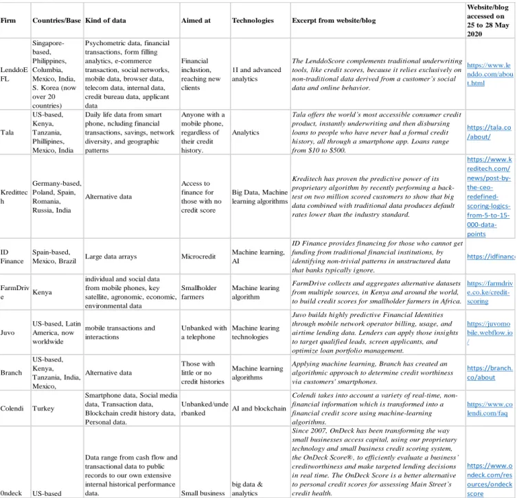
We note that our model has links to what is happening today in the real world of using artificial intelligence and data analytics for credit scoring. Table 4 provides examples of some lenders who are using credit scoring, often aimed at small businesses, microcredit or financially excluded people. Many of them indicate on their website that they are using alternative data to the traditional financial or operating data. This has been made possible with new technologies. We also take an excerpt from each website to indicate the use or impact of their work, as claimed by them.
Insert table 4 about here
Moreover, most researchers indicate that the lender proposes successive loans with increasing size as an incentive mechanism to improve the profit. However, our analysis in part 5 shows that this incentive will not motivate the borrower if the production function does not allow greater income, i.e., if the
business is not scalpel beyond K∗. Therefore, borrowers may prefer not to graduate to successive lending states. Formally, we propose
Proposition 1: There is a range of loan sizes where progressive lending works. The upper limit of this range depends upon the borrower characteristics as well as the production function.
We have noted that the rational borrower of our type may prefer to default in many situations. However, owing to moral and social considerations, they may not default, leading to high stress and even suicides emanating from shame (Ashta, Khan, and Otto 2015; Karim 2008). Future research can factor in these considerations for understanding why borrowers default. Part 6 shows that this action of the
borrower may affect the microfinance institution’s objective of financial inclusion.
Certainly, the qualitative evaluation of the probability to default or reimburse depends on many variables. However, if we have data, a future researcher could run a Cox regression which would validate our model by estimating the probability of default or reimbursement connected to different variables (gender, family conditions and obligations, the objective to improve busin ess, education and many other). With such a model, the MFI can draw a prototype of ideal borrowers who would get to inclusion and detect the weak points in the chain which deserve attention to avoid default.
We have already indicated that with the development of artificial intelligence and machine learning, these issues will increasingly be incorporated in credit scoring models for decision -making. Our study suggests that in addition to these borrower characteristics, the lender may also be able to incorpor ate borrower’s production function in his lending strategy, which should also be possible with the
development of artificial intelligence and machine learning. In fact, AI and machine learning may also refine the estimated production functions over time.
We note that our model is limited to entrepreneurial lending where successive loans can be repaid by higher incomes: it is not applicable to consumer microlending.
Agier, Isabelle, and Ariane Szafarz. (2013). "Microfinance and Gender: Is There a Glass Ceiling on Loan Size?" World Development 42: 165-181.
https://doi.org/https://doi.org/10.1016/j.worlddev.2012.06.016.
Akerlof, George A. (1970). "The Market for "Lemons": Quality Uncertainty and the Market Mechanism."
Quarterly Journal of Economics 84 (3): 488-500..
Akula, Vikram. (2010). A Fistful of Rice: My Unexpected Quest to End Poverty Through Profitability. Boston, MA: Harvard Business Press.
Allison, Thomas H., Blakley C. Davis, Jeremy C. Short, and Justin W. Webb. (2015). "Crowdfunding in a Prosocial Microlending Environment: Examining the Role of Intrinsic Versus Extrinsic Cues. ."
Entrepreneurship: Theory & Practice 39 (1): 53-73.
Armendàriz, Beatriz, and Jonathan Morduch. (2010). The Economics of Microfinance. Cambridge, MA: MIT Press.
Ashta, Arvind, Karl Dayson, Rajat Gera, Samanthala Hettihewa, N.V. Krishna, and Christopher Wright. (2013). "Microcredit as a Social Innovation." In The International Handbook on Social Innovation, edited by Frank Moulaert, Diana MacCallum, Abid Mehmood and Abdelillah Hamdouch, 80-92. Cheltenham, UK.: Edward Elgar.
Ashta, Arvind, Saleh Khan, and Philipp E. Otto. (2015). "Does Microfinance Cause or Reduce Suicides? Policy Recommendations for Reducing Borrower Stress." Strategic Change: Briefings in
Entrepreneurial Finance 24 (2): 165–190.
Assadi, Djamchid, ed. (2016). Strategic Approaches to Successful Crowdfunding. Hershey, PA: IGI Global. Attuel-Mendes, Laurence. (2014). "Crowdfunding platforms for microfinance: a new way to eradicate
poverty through the creation of a global hub?" Cost Management 28 (2): 38-47. Banerjee, Saugata, and Olivier Cadot. (1996). "Syndicated lending under asymmetric creditor
information." Journal of Development Economics 49 (2): 289-306.
Baulia, Susmita. (2019). "Take-up of joint and individual liability loans: An analysis with laboratory experiment." Journal of Behavioral and Experimental Economics 82: 101456.
https://doi.org/https://doi.org/10.1016/j.socec.2019.101456.
Besley, T., and S. Coate. (1995). "Group lending, repayment incentives and social collateral." Journal of
Development Economics 46: 1-18.
Bond, Philip, and Ashok S. Rai. (2009). "Borrower runs." Journal of Development Economics 88 (2): 185-191. https://doi.org/https://doi.org/10.1016/j.jdeveco.2008.06.005.
Bumacov, Vitalie, Arvind Ashta, and Pritam Singh. (2014). "The Use of Credit Scoring in Microfinance Institutions and Their Outreach " Strategic Change: Briefings in Entrepreneurial Finance 23 (7-8). ---. (2017). "Credit scoring: A historic recurrence in microfinance." Strategic Change 26 (6): 543-554.
https://doi.org/10.1002/jsc.2165.
Caste, Nicholas J. (1992). "Drug Testing and Productivity." Journal of Business Ethics 11 (4): 301-306. Crosman, Penny. (2017). "Behind Credit Suisse’s foray into microlending to the global poor." American
Banker. https://www.americanbanker.com/news/behind-credit-suisses-foray-into-microlending-to-the-global-poor.
de Meza, David, and David Webb. (2000). "Does credit rationing imply insufficient lending?" Journal of
Public Economics 78 (3): 215-234. https://doi.org/https://doi.org/10.1016/S0047-2727(99)00099-7..
Demirgüç-Kunt, Asli, Leora Klapper, Dorothe Singer, Saniya Ansar, and Jake Hess. (2018). The Global
Findex Database 2017: Measuring Financial Inclusion and the Fintech Revolution. World Bank
(Washington, DC: World Bank).
https://globalfindex.worldbank.org/sites/globalfindex/files/2018-04/2017%20Findex%20full%20report_0.pdf.
Dowla, Asif, and Dipal Barua. (2006). The poor always pay back: The Grameen II story. Bloomfield, CT: Kumarian Press.
Egli, Dominik. (2004). "Progressive Lending as an Enforcement Mechanism in Microfinance Programs."
Review of Development Economics 8 (4): 505-520. 10.1111/j.1467-9361.2004.00249.x
Elkington, John, Jed Emerson, and Seb Beloe. (2006). "The Value Palette: A Tool For Full Spectrum Strategy." California Management Review 48 (2): 6-28.
http://search.ebscohost.com/login.aspx?direct=true&db=bth&AN=19902360&site=ehost-live. Gershkov, Alex, Benny Moldovanu, and Philipp Strack. (2018). "Revenue-Maximizing Mechanisms with
Strategic Customers and Unknown, Markovian Demand." Management Science 64 (5): 2031-2046. https://doi.org/10.1287/mnsc.2017.2724..
Ghatak, M. (1999). "Group Lending, Local Information, and Peer Selection." Journal of Development
Economics 60 (6): 27-51.
Ghosh, Suman, and Eric Van Tassel. (2013). "Funding microfinance under asymmetric information."
Journal of Development Economics 101: 8-15.
Guttman, Joel M. (2008). "Assortative matching, adverse selection, and group lending." Journal of
Development Economics 87: 51-56.
Hardeman, B. (2012). "Lenddo's Social Credit Score: How Who You Know Might Affect Your Next Loan." Accessed April 1, 2020.
Hyun, Junghwan, and Azad Uddin. (2016). "Heterogeneous lending behaviors and gross loan flows in developing economies." Economic Modelling 55: 359-372.
https://doi.org/https://doi.org/10.1016/j.econmod.2016.02.024..
Ibrahim, Rouba, Mor Armony, and Achal Bassamboo. (2017). "Does the Past Predict the Future? The Case of Delay Announcements in Service Systems." Management Science 63 (6): 1762-1780.
https://doi.org/10.1287/mnsc.2016.2425..
INSEE. (2012). Taux de survie en 2011 des entreprises créées en 2006 selon le secteur d'activité :
comparaisons régionales. INSEE (France).
Iyengar, Kishen Parthasarathy , Najam Ahmad Quadri, and Vikas Kumar Singh. (2010). "Information Technology and Microfinance Institutions: Challenges and Lessons Learned." Journal of Electronic
Commerce in Organization 8 (2): 1-11.
Karim, Lamia. (2008). "Demystifying Micro-Credit: The Grameen Bank, NGOs, and Neoliberalism in Bangladesh." Cultural Dynamics 20 (1): 5-29. https://doi.org/10.1177/0921374007088053.. Kessler, Denis, and André Masson. (1989). "Bequest and Wealth Accumulation: Are Some Pieces of the
Puzzle Missing?" Journal of Economic Perspectives 3 (3): 141-152..
Khan, Saleh, and Arvind Ashta. (2012). "Cost control in Microfinance: Lessons from the ASA case." Cost
Management 26 (1): 5-22.
Li, Lin Yang, Niels Hermes, and Aljar Meesters. (2019). "Convergence of the performance of microfinance institutions: A decomposition analysis." Economic Modelling 81: 308-324.
https://doi.org/https://doi.org/10.1016/j.econmod.2019.05.014.
Lucas, J. R. Robert E. (2003). "Macroeconomic Priorities." American Economic Review 93 (1): 1-14.
http://search.ebscohost.com/login.aspx?direct=true&db=bth&AN=9467558&site=ehost-live. Mahmood, Samia, Javed Hussain, and Harry Z. Matlay. (2014). "Optimal microfinance loan size and
poverty reduction amongst female entrepreneurs in Pakistan." Journal of Small Business and
Enterprise Development 21 (2): 231-249.
Makridakis, Spyros. (2017). "The forthcoming Artificial Intelligence (AI) revolution: Its impact on society and firms." Futures 90: 46-60. https://doi.org/https://doi.org/10.1016/j.futures.2017.03.006. Mallick, Debdulal, and Munirul H. Nabin. (2018). "Cost effectiveness or serving the poor? Factors
determining program placement of NGOs in Bangladesh." Economic Modelling 69: 281-290.
Mankiw, N. Gregory. (2013). "Defending the One Percent." Journal of Economic Perspectives 27 (3): 21-34. https://doi.org/10.1257/jep.27.3.21.
Margolis, Howard. (1982). "A thought experiment on demand-revealing mechanisms." Public Choice 38 (1): 87-91.
Morawczynski, Olga. (2011). "Saving through the mobile: A study of M-PESA in Kenya." In Advanced
Technologies for Microfinance: Solutions and Challenges, edited by Arvind Ashta. Hershey, PA:
IGI Global.
Pansera, Mario, Melf-Hinrich Ehlers, and Christian Kerschner. (2019). "Unlocking wise digital techno-futures: Contributions from the Degrowth community." Futures 114: 102474.
https://doi.org/https://doi.org/10.1016/j.futures.2019.102474. Rawls, J. (1971). A Theory of Justice. Cambridge: Harvard University Press.
Rosenberg, Richard, Adrian Gonzalez, and Sushma Narain. (2009). The New Moneylenders: Are the Poor
Being Exploited by High Microcredit Interest Rates? CGAP (Washington, D.C.).
Schulte, Markus, and Adalbert Winkler. (2019). "Drivers of solvency risk – Are microfinance institutions different?" Journal of Banking & Finance 106: 403-426.
https://doi.org/https://doi.org/10.1016/j.jbankfin.2019.07.009.
Shankar, Savita. (2007). "Transaction costs in group microcredit in India." Management Decision 45 (8): 1331-1342. 10.1108/00251740710819069
Shapiro, DA. (2015). "Microfinance and dynamic incentives." Journal of Development Economics 115: 73-84.
Shrivastava, Prateek. (2010). "Build it - Will They Come? A Study of the Adoption of Mobile Financial Services by Low Income Clients in South Africa." Journal of Electronic Commerce in Organizations 8 (3): 1-14. 10.4018/jeco.2010070101
Singh, Vijeta, and Puja Padhi. (2017). "Dynamic Incentives and Microfinance Borrowers:A Comparative Study of Self-help Groups and Joint Liability Groups: A Case Study of Mirzapur District in India."
Journal of Land and Rural Studies 5 (1): 67-92. https://doi.org/10.1177/2321024916677609. Soltane Bassem, Ben. (2014). "Total factor productivity change of MENA microfinance institutions: A Malmquist productivity index approach." Economic Modelling 39: 182-189.
https://doi.org/https://doi.org/10.1016/j.econmod.2014.02.035. Stiglitz, Joseph E., and Andrew Weiss. (1981). "Credit Rationing in Markets with Imperfect Information." American Economic
Review 71 (3): 393-410.
Tedeschi, Gwendolyn Alexander. (2006). "Here today, gone tomorrow: Can dynamic incentives make microfinance more flexible?" Journal of development Economics 80 (1): 84-105.
Van Tassel, Eric. (1999). "Group lending under asymmetric information." Journal of Development
Economics 60 (1): 3-25.
WEF. (2019). The New Physics of Financial Services – How artificial intelligence is transforming the
financial ecosystem. World Economic Forum. https://www.weforum.org/reports/the-new-physicsof-financial-services-how-artificial-intelligence-istransforming-the-financial-ecosystem. Wempe, Ben. (2008). "Four Design Criteria for any Future Contractarian Theory of Business Ethics."
Journal of Business Ethics 81 (3): 697-714. https://doi.org/10.1007/s10551-007-9542-x. Yunus, Muhammad. (2003). Banker to the Poor: Micro-Lending and the Battle Against World Poverty.
New York: Public Affairs.
Zhang, Zhe George. (2009). "Performance Analysis of a Queue with Congestion-Based Staffing Policy."
Figure 1: Markov chain describes the dynamic of the borrower’s strategy depending on her profit probabilities α and the perception of the probability of a second chance γ, Source: Authors
Figure 2: Markov chain illustrates borrower-strategy with different possibilities in each state (succeed, stay, recede, or exclude) along with intermediate possibility of second chance. Source: Authors
Figure 3: Earnings (Y) and Consumption (C) functions for a small business Source: Authors
Figure 8: Expected profit (z) with possibility of advancing, staying in the same state retreating to a previous state. Source: Authors
Table 1: Average loan size in microfinance (2010-2018) in US dollars Average loan balance per
borrower (USD)
2010 2012 2014 2016 2018
Africa 743 830 1055 937 1351
East Asia and the Pacific 1055 1380 1251 1810 1777
Eastern Europe and Central Asia 3299 3422 3726 2415 2802 Latin America and The Caribbean 1720 1946 2236 2269 2555
Middle East and North Africa 933 839 905 877 1077
South Asia 237 226 223 276 347
Grand Total 1410 1553 1714 1541 1839
Source: Based on MIX data downloaded on March 18, 2020, after filtering out balances over $30,000. The number of MFIs reporting this data declined from 1381 in 2010 to 684 in 2018.
Table 2 Portfolio at risk (30 days) of microfinance institutions (2010-2018) 2010 2012 2014 2016 2018 Sample Size (number of MFIs) 1058 906 932 716 644 Minimum 0.00% 0.00% 0.00% 0.00% 0.00% First Quartile 1.51% 1.26% 1.19% 1.73% 1.60% Median 4.18% 3.81% 3.70% 4.56% 4.07% Average 8.00% 7.05% 5.83% 8.39% 7.17% Third Quartile 9.33% 7.68% 6.59% 8.64% 7.66% Maximum 99.40% 97.74% 98.57% 98.70% 99.64%
Table 3: Alternative probabilities of success and second chance Success probability Second
Chance Probability
Low Intemediate High
Low Case 3 (0.25, 0.25, 0.25, 0.20) Intermediate Case 4 (0.5, 0.7, 0.8, 0.4) High Case 1 (0.25, 0.25, 0.25, 0.75) Case 2 (0.25, 0.50, 0.25, 0.75) Source: Authors
Table 4: Credit scoring applications
Source: Authors, different websites last accessed on June 16, 2020. Firm Countries/Base Kind of data Aimed at Technologies Excerpt from website/blog
Website/blog accessed on 25 to 28 May 2020 LenddoE FL Singapore-based, Philippines, Columbia, Mexico, India, S. Korea (now over 20 countries)
Psychometric data, financial transactions, form filling analytics, e-commerce transaction, social networks, mobile data, browser data, telecom data, internal data, credit bureau data, applicant data Financial inclustion, reaching new clients 1I and advanced analytics
The LenddoScore complements traditional underwriting tools, like credit scores, because it relies exclusively on non-traditional data derived from a customer’s social data and online behavior.
https://www.le nddo.com/abou t.html Tala US-based, Kenya, Tanzania, Phillipines, Mexico, India
Daily life data from smart phone, ncluding financial transactions, savings, network diversity, and geographic patterns Anyone with a mobile phone, regardless of their credit history. Analytics
Tala offers the world’s most accessible consumer credit product, instantly underwriting and then disbursing loans to people who have never had a formal credit history, all through a smartphone app. Loans range from $10 to $500. https://tala.co /about/ Kredittec h Germany-based, Poland, Spain, Romania, Russia, India Alternative data Access to finance for those with no credit score
Big Data, Machine learning algorithms
Kreditech has proven the predictive power of its proprietary algorithm by recently performing a back-test on two million scored customers to show that big data combined with traditional data produces default rates lower than the industry standard.
https://www.k reditech.com/ news/post-by- the-ceo- redefined- scoring-logics- from-5-to-15- 000-data-points ID Finance Spain-based,
Mexico, Brazil Large data arrays Microcredit
Machine learning, AI
ID Finance provides financing for those who cannot get funding from traditional financial institutions, by identifying non-trivial patterns in unstructured data that banks typically ignore.
https://idfinance.com/sustainability/
FarmDriv
e Kenya
individual and social data from mobile phones, key satellite, agronomic, economic, environmental data
Smallholder farmers
Machine learing algorithm
FarmDrive collects and aggregates alternative datasets from multiple sources, in Kenya and around the world, to build credit scores for smallholder farmers in Africa.
https://farmdriv e.co.ke/credit-scoring Juvo US-based, Latin America, now worldwide
mobile transactions and interactions
Unbanked with a telephone
Machine learing technologies
Juvo builds highly predictive Financial Identities through mobile network operator billing, usage, and airtime lending data. Lenders can apply those insights to target qualified leads, screen applicants, and optimize loan portfolio management.
https://juvomo bile.webflow.io / Branch US-based, Kenya, Tanzania, India, Mexico, Alternative data Those with little or no credit histories Machine learning algorithms
Applying machine learning, Branch has created an algorithmic approach to determine credit worthiness via customers' smartphones.
https://branch. co/about
Colendi Turkey
Smartphone data, Social media data, Transaction data, Blockchain credit history data, Personal data.
Unbanked/unde
rbanked AI and blockchain
Colendi takes into account a variety of real-time, non-financial information which is transformed into a financial credit score using machine-learning algorithms.
https://www.co lendi.com/faq
0ndeck US-based
Data range from cash flow and transactional data to public records to our own extensive internal historical performance
data. Small business
big data & analytics
Since 2007, OnDeck has been transforming the way small businesses access capital, using our proprietary technology and small business credit scoring system, the OnDeck Score®, to efficiently evaluate a business’ creditworthiness and make targeted lending decisions in real time. The OnDeck Score is a better alternative to personal credit scores for assessing Main Street’s credit health.
https://www.o ndeck.com/res ources/ondeck score