Algorithmical and mathematical approaches of causal graph dynamics

(1)

HAL Id: tel-01188690

https://tel.archives-ouvertes.fr/tel-01188690

Submitted on 31 Aug 2015

HAL is a multi-disciplinary open access

archive for the deposit and dissemination of sci-entific research documents, whether they are pub-lished or not. The documents may come from teaching and research institutions in France or abroad, or from public or private research centers.

L’archive ouverte pluridisciplinaire HAL, est destinée au dépôt et à la diffusion de documents scientifiques de niveau recherche, publiés ou non, émanant des établissements d’enseignement et de recherche français ou étrangers, des laboratoires publics ou privés.

Algorithmical and mathematical approaches of causal

graph dynamics

Simon Martiel

To cite this version:

Simon Martiel. Algorithmical and mathematical approaches of causal graph dynamics. Other [cs.OH]. Université Nice Sophia Antipolis, 2015. English. �NNT : 2015NICE4043�. �tel-01188690�

(2)

UNIVERSIT´

E NICE SOPHIA ANTIPOLIS

ECOLE DOCTORALE STIC

SCIENCES ET TECHNOLOGIES DE L’INFORMATION ET DE LA COMMUNICATION

TH`

ESE

pour l’obtention du grade de

Docteur en Sciences

de l’Universit´e Nice Sophia Antipolis Mention: Informatique

pr´esent´ee et soutenue par

Simon MARTIEL

Approches informatique et math´

ematique

des dynamiques causales de graphes

Th`ese dirig´ee par Pablo ARRIGHI et Bruno MARTIN soutenue le 6 juillet 2015

Jury :

M. Pablo ARRIGHI Université Aix-Marseille Directeur de thèse M. Bruno MARTIN Université Nice Sophia Antipolis Directeur de thèse

M. Vincent DANOS CNRS Rapporteur

M. Emmanuel JEANDEL Universit´e de Lorraine Rapporteur M. Jarkko KARI University of Turku Rapporteur

M. Gilles DOWEK INRIA Examinateur

M. Jean-Louis GIAVITTO CNRS Examinateur M. Eric GOLES Universidad Adolfo Ib´a˜nez Examinateur

(3)

Abstract

English

Cellular Automata constitute one of the most established model of discrete physical transformations that accounts for euclidean space. They implement three fundamental symmetries of physics: causality, homogeneity and finite density of information. Even though their origins lies in physics, they are widely used to model spatially distributed computation (self-replicating ma-chines, synchronization problems,...), as well as a great variety of multi-agents phenomena (traffic jams, demographics,...). While being one of the most studied model of distributed computation, their rigidity forbids any trivial extension toward time-varying topology, which is a fundamental requirement when it comes to modelling phenomena in biology, sociology or physics: for instance when looking for a discrete formulation of general relativity. Causal graph dynamics generalize cellular automata to arbitrary, bounded degree, time-varying graphs. In this work, we generalize the fundamental structure results of cellular automata for this type of transformations. We endow our graphs with a compact metric space structure, and follow two approaches. An axiomatic approach based on the notions of continuity and shift-invariance, and a constructive approach, where a local rule is applied synchronously on every vertex of the graph. Compactness allows us to show the equivalence of these two definitions, extending the famous result of Curtis-Hedlund-Lyndons theorem. Another physics-inspired symmetry is then added to the model, namely reversibility. We answer the question whether the inverse of a causal graph dynamics is itself a causal graph dynamics, and prove the existence of a block decomposition of reversible causal graph dynamics, thereby gen-eralizing two results of reversible cellular automata theory. We present the construction of a family of intrinsically universal local rules, indexed by the degree of the simulated rule, such that every local rule can be simulated by

(4)

2

one of these rules, with a constant delay, whilst preserving the space-time structure of the computation. We also present the construction of a universal construction machine, able to construct any instance of causal graph dynam-ics. Finally, we provide a correspondence between graphs and ∆−complexes, allowing us to define causal dynamics of discrete geometrical spaces.

Fran¸cais

Le modèle des automates cellulaires constitue un des modèles le mieux établi de physique discrète sur espace euclidien. Ils implantent trois symétries fon-damentales de la physique: la causalité, l’homogénéité et la densité finie de l’information. Bien que l’origine des automates cellulaires provienne de la physique, leur utilisation est très répandue comme modèles de calcul distribué dans l’espace (machines auto-réplicantes, problèmes de synchro-nisation,...), ou bien comme modèles de systèmes multi-agents (congestion du trafic routier, études démographiques,...). Bien qu’ils soient parmis les modèles de calcul distribué les plus étudiés, la rigidité de leur structure in-terdit toute extension triviale vers un modèle de topologie variant dans le temps, qui se trouve être un prérequis fondamental à la modélisation de cer-tains phénomènes biologiques, sociaux ou physiques, comme par exemple la discrétisation de la relativité générale.

Les dynamiques causales de graphes généralisent les automates cellulaires aux graphes arbitraires de degré borné et pouvant varier dans le temps. Dans cette thèse, nous nous attacherons à généraliser certains des résultats fonda-mentaux de la théorie des automates cellulaires. En munissant nos graphes d’une métrique compacte, nous présenterons deux approches différentes du modèle. Une première approche axiomatique basée sur les notions de conti-nuité et d’invariance par translation, et une deuxième approche constructive, où une règle locale est appliquée en parallèle et de manière synchrone sur l’ensemble des sommets du graphe. La compacité nous permettra de prou-ver l’équivalence entre ces deux définitions, étendant le célèbre résultat de Curtis, Hedlund et Lyndon sur les automates cellulaires. Nous ajouterons ensuite une symmétrie supplémentaire au modèle: la réversibilité. Nous répondrons à la question de savoir si toute instance bijective de notre modèle admet bien une dynamique inverse, et nous montrerons comment toute in-stance réversible peut être décomposée en un circuit d’opérations locales et réversibles. Nous présenterons la construction d’une famille de règles locales

(5)

3 intrinsèquement universelles, indexées selon le degré de la règle simulée, et capables de simuler toute autre instance du modèle, tout en préservant la structure spatio-temporelle du calcul. Ce résultat nous permettra ensuite de décrire une machine de construction universelle capable de construire n’importe quelle instance du modèle. Enfin nous étudierons une correspon-dance entre graphes et ∆−complexes nous permettant ainsi de définir les dynamiques causales d’espaces géométriques discrets.

(6)

(7)

Remerciements

Je voudrais commencer par remercier mes deux directeurs de thèse, Pablo et Bruno. Pablo pour m’avoir fait découvrir le monde merveilleux de la recherche, la richesse des interactions entre physique et informatique et surtout pour avoir pris le temps de s’occuper d’un étudiant qui est arrivé dans son bureau, il y a maintenant six ans, en lui demandant un sujet de stage en in-formatique quantique. Bruno pour avoir accepté de m’encadrer sur un sujet original, pour s’être prêté au jeu des dynamiques causales de graphes et pour avoir pris le temps de relire ma thèse avec autant d’attention.

Je voudrais ensuite remercier les membres de l’équipe MC3: Enrico (pour m’avoir concocté un Master de rêve), Sandrine (si Bruno est mon “père de thèse”, Sandrine est sans aucun doute ma “mère de thèse”), Christophe (pour les discussion de relativité, les jeux vidéos, et les groupes de travail sur les grands ordinaux), mon co-bureau Pierre-Alain (pour les longues discussions autout d’un thé), ainsi que ceux de passage: Émilie, Jonas et Fabien.

Je me dois de remercier mes trois rapporteurs qui ont accepté de relire cette thèse: Vincent Danos, Emmanuel Jeandel et Jarkko Kari, ainsi que mes examinateurs Jean-Louis Giavitto, Gilles Dowek et Éric Golès.

Je voudrais remercier toutes ces personnes qui ont croisé ma route au cours de ces dernières années, et avec qui j’ai eu l’occasion de collaborer ou simplement de discuter: Kevin Perrot, Simon Perdrix, Zizhu Wang, Vincent Nesme, Eric Thierry, Pascal Vanier, Maxime Senot.

Enfin, je voudrais remercier tous ceux qui m’ont supporté pendant mes études, en particulier les ex-lyonnais, Bruno, Guilhem, Florent, Étienne, Alexis, ainsi que les ni¸cois, Julien, Damien et Mug.

Et pour finir ceux qui me supportent ou m’ont supporté au quotidien, ma famille, et surtout Elsa pour sa bravoure sans égale face à mon bordel constant.

(8)

(9)

Chapter 1 Introduction

Interactions between theoretical physics and computer science are often de-scribed as unilateral. Either physicists require some algorithmic knowledge to simulate some natural phenomenon, or computer scientists use different phys-ical theories to design new computational models and study their properties. It seems, however, that the interaction between those two fields could lead to a more profound dialogue. It turns out that the current trend in theoretical physics is to identify physical systems to the ’information’ they carry, and not by the ’matter’ they are constituted of. In fact, this vision can be directly traced back to the postulates of different physical theories. For instance, the notion of entropy, present in thermodynamics, captures the notion of “quan-tity of information” inside a closed physical system. There is a growing opin-ion that physics will soon enter a ‘computatopin-ional’ trend. Taking this view to an extreme in this direction, one could imagine making the Gedankenexper-iment that the universe is nothing but a large parallel computer, processing bits of information rather than mechanical processes: this is the “digital physics” paradigm. This vision was proposed by numerous great researchers, such as Fredkin, Toffoli and Margolus [Fre92, FT82, Mar88, Mar84].

One of the most famous computation model born thanks to this approach of physics is the model of cellular automata. This model, introduced by von Neumann and Ulam in the forties, is the simplest discrete model captur-ing three fundamental symmetries of physics: causality (information travels with a bounded speed across space), homogeneity (the laws of physics are the same everywhere, at every time) and bounded density of information (a bounded volume of space cannot contain an unbounded amount of in-formation). In their primary definition, cellular automata consist in arrays

(12)

10 CHAPTER 1. INTRODUCTION

of cells, each of them containing a state in a finite set. The arrays evolve synchronously and in discrete time steps, the state of each cell being up-dated according to the states of its neighbours. In a more computer science oriented-vision, cellular automata can be seen as the synchronous applica-tion of a local rule throughout the grid. Later, in 1969, Hedlund, together with Curtis and Lyndon, gave a mathematical reality to the model by prov-ing that cellular automata defined usprov-ing local rules are, in fact, uniformly continuous and shift-commuting transformations over a set of configurations. This plurality of the formalisms places this model directly at the interface between physics, mathematics and computer science. However, the rigidity of the underlying space is often cited as a limitation of the model. Indeed, while they are the perfect choice when considering dynamics on Euclidean space, they fail to model dynamics over irregular topologies, like for instance general discrete metric spaces, or arbitrary interaction agent networks. Cel-lular automata have been generalized in many flavours. Some generalizations explore the way a cellular automaton can act upon its set of configurations, such as asynchronous cellular automata, while others try to generalize the configurations space. For instance, it is possible to nicely generalize cellular automata to act upon Cayley graphs. A Cayley graph is a graph representing a finitely generated group: each vertex of the graph represents an element of the group, and for each relation a · b = c where b is a generator, an edge between vertices a and c is added, labelled with b at one end and b−1 _{at the}

other. These graphs have the nice feature of being very regular: all vertices have the same degree and are indistinguishable, making it easy to generalize the notion of cellular automata acting upon them. Even though this general-ization allows the definition of cellular automata acting upon a much relaxed set of configuration, the underlying space is still regular and fixed in time.

However, there are many situations where the interaction of some agents (for instance some particles, some computer process, or some biological agent) according to some interactions networks, leads to a change in the network itself. A good example would be a network composed of people and their address books. The interaction network would change locally (e.g. you could share your contacts with one of your friend), or maybe a new person could enter the network. Another, more physical, example would the case of general relativity. In this case, the network would represent space itself, with its curvature. Some massive particle will then move across space along the path dictated by its curvature. The motion of the particle will, in turn, modify space curvature, thus modifying the underlying network. Modelling those

(13)

11 dynamics require a less restricted, time-varying interaction network. There have been several approaches to generalize cellular automata not just to Cayley graphs, but to arbitrary connected graphs of bounded degree, with, sometimes, time-variation of the topology:

• With a fixed, arbitrary topology, in order to describe certain distributed algorithms [PR02, DMG08, Gru10], or to generalize the Garden-of-Eden theorem [Gro99, CSS04].

• Through the simulation environments of [GS08, VMPDJ11, KKBS05] which offer the possibility of applying a local rewriting rule simultane-ously in different non-conflicting places.

• Through concrete instances advocating the concept of cellular automata extended to time-varying graphs as in [TKM09, KK07, KCN+_{10], some}

of which are advanced algorithmic constructions [TKM02, TMKK05]. • Through amalgamated graph transformations [BFH87, L¨ow93] and

par-allel graph transformations [EL93, Tae96, Tae97], which work out rig-orous ways to apply a local rewriting rule synchronously throughout a graph.

• Through rule-based graph rewriting languages [DL04], or their stochas-tic versions [DFF+_12].

The approach of this thesis is different in the sense that it first generalizes Cayley graphs and then applies the mathematical characterization of cellu-lar automata as the set of shift-invariant continuous transformations in order to generalize cellular automata, thus defining a new model: Causal Graph Dynamics. Compared to the above cellular automata approaches, our model extends the fundamental structure theorems about cellular automata to ar-bitrary, connected, bounded degree, time-varying graphs. Compared with the above mentioned graph rewriting papers, the contribution is to deduce aspects of amalgamated/parallel graph transformations from the axiomatic and topological properties of the global function.

The subject of this thesis is to study and develop this model, which was first introduced by Arrighi and Dowek in [AD12]. In this first version, the authors already achieved an extension of cellular automata to arbitrary, bounded degree, time-varying graphs, although through a notion of conti-nuity, with the same motivations. However, this work failed to endow the

(14)

configuration space with a compact metric, necessary to the formulation of a similar result as Hedlund’s theorem, and the existence of such a metric was left as an open question. It also leaves open whether causal graph dynamics are (locally) computable. Indeed, in this early formalization of the model, the graph structure used to define the configuration space of the cellular au-tomata had identified vertices. The shift-invariance of a graph transformation was then naturally translated as a weak commutation with renamings of the vertices. While this allows a relatively compact definition for shift-invariance, it does not prevent the graph transformation to hide possibly uncomputable functions inside the identifiers of the vertices. In order to tackle this issue, we had to define a new model of graph, where vertices have no identifier whatsoever.

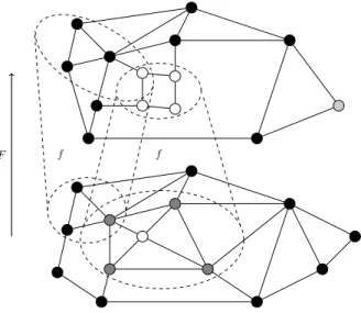
This thesis is organized as follows. Chapter 2 is dedicated to the construction of this model of graph. The introduction of this new model of graph allows to define our model of causal graph dynamics as graph transformations satisfy-ing three properties: continuity, shift-invariance and boundedness. Alterna-tively, these transformations can also be defined as the synchronous mapping of a local rule on every vertex of a graph (see Figure 1.1).

These two definitions and their equivalence are presented in Chapter 3, thus generalizing Hedlund’s theorem. We will then focus on an additional symmetry almost omnipresent in physics: reversibility. Given the variety of results in reversible cellular automata theory, it seems quite natural to study this additional property when considering extension of cellular automata. More particularly, the fact that causal graph dynamics can, for instance, change the number of vertices of a graph brings novel questions. Another, more physical, motivation is the design of a quantum version of causal graph dynamics, which is yet to achieve. Several aspects of this symmetry are addressed in chapter 4. First, the correspondence between invertibility and reversibility is studied. Then, a decomposition of reversible causal graph dynamics into bounded-depth circuit of reversible local gates is presented. Another fructifying area of discrete computational models is the study of their universality. Intrinsic universality, in particular, is a subject of choice. This type of universality explores the capacity of the model to simulate it-self efficiently, and has been intensively studied for cellular automata and their various extensions. In the scope of studying a computational model as a physical toy model, the quest of the simplest universal instance of the model takes a completely new meaning, and could help us understand the true structure of physical laws. Another, less common, form of universality

(15)

13

f

F f

Figure 1.1: Representation of a graph transformation F induced by the homogeneous and synchronous application of a local rule f on every vertex of a graph.

is von Neumann’s notion of universal construction machine, where a machine can read a description of any instance of the model and build this instance. Chapter 5 provides a natural definition of intrinsic universality and describes the construction of a family of intrinsically universal local rules, together with a universal construction machine. A natural application of causal graph dy-namics to physics is the modelling of discrete version of general relativity. Even though this model seems adequate, in terms of structure of the dynam-ics, to the study of this complicated field, the structure of the configuration space is still too relaxed to be considered as a discrete geometrical space. Chapter 6 explores a correspondence between generalized Cayley graphs and ∆-complexes which leads, in the two-dimensional case, to a definition of dis-crete surface causal dynamics.

(16)

How to read this thesis?

Even though the origin of causal graph dynamics model lies in physics, I was conducted to study very different aspects of this model, some of which have nothing to do with constructing a discrete model able to embed the power of relativity. Here are some guidelines to read this thesis. Although Chapter 2 and 3 are mandatory to get the basic definitions of the model, a reader having no particular interest in the axiomatic approach of the model might want to focus its reading on sections 2.1, and 3.2, which provides sufficient background to understand the universal construction of Chapter 5. On the other hand, a reader whose interest lies in the reversibility of CGD, and in particular the relations between invertibility and reversibility, might want to skip the details of the local rule construction, as it is not a requirement for the results of Chapter 4.

(17)

Chapter 2 Generalized cayley graphs

Classical graphs. In the original work of Arrighi and Dowek [AD12], the model of causal graph dynamics was based on what we could refer to as “usual” graphs, with the added feature of using ports to name the neigh-bours of a vertex and having a bound on the degree of the graph. This model is sufficient to define cellular automata over time-varying graphs. In order to define local rules over graphs, the authors needed to use identifiers in vertices. The influence of those identifiers was then limited by enforcing a weakened commutation relation between the cellular automaton and any renaming of the vertices. Even though the intricacies of these identifiers was sort of decoupled from the rest of the evolution, this still made it impossible to prove that applying a causal graph dynamics to a finite graph was a com-putable process, which seemed to be a desirable property. It became natural to try to embed this absence of influence of the identifiers, by just removing these identifiers right from the start in the graph model itself, rather than “artificially” removing them when defining the cellular automata.

Cayley graphs. Cayley graphs are directed graphs, or digraphs, encoding a finitely generated group. The Cayley graph of a group having a set of gen-erators S = {s1, s−11 , ..., sn, s−1n } is a graph whose vertices are the elements

of the group and whose edges are of the form (g, g · s) where s ∈ S and · denotes the group operation. The regularity of these graphs allows to eas-ily generalize the classical definition of cellular automata by replacing the n−dimensional Euclidean grid topology by a Cayley graph. One interesting feature of these graphs is the fact that, even though their vertices are labelled by an element of the group, one does not need this information to refer to a

(18)

16 CHAPTER 2. GENERALIZED CAYLEY GRAPHS

precise vertex. Indeed one could imagine referring to a vertex by using the sequence of edges we need to traverse to reach it, starting from the identity. To go even further, we might want to fully describe the target vertex, and give the set of all paths starting from the identity and leading to it. In fact this representation is equivalent to describe the group as a language over he set of its generators S considered as a finite alphabet, together with an equivalence relation induced by the group equality.

Generalized Cayley graphs. Now consider a “classical” graph where a vertex is pointed. Even though it is not a Cayley graph, we can still describe a vertex of this graph by using the set of paths starting from the pointed vertex and leading to it. Using ports to number the adjacent edges of the vertices, each path can be seen as a word over the alphabet of the ports and the set of all paths as a language. We can still quotient this language by the relation “lead to the same vertex”. The corresponding structure is not necessarily a group, but can represent any “classical” graph. This structure is what we call a generalized Cayley graph.

The content of this chapter is based on [AMN13] and [AM12], co-authored with Pablo Arrighi and Vincent Nesme.

2.1 Brief overview.

This first section offers a brief overview of the model of generalized Cayley graph (or pointed graph modulo) used in this thesis. Sections 2.2, 2.3 and 2.4 provide the formal definition of the graph model and its properties. Finally, appendix A provides all the details and interpretations of this model. Pointed graph modulo. Basically, the pointed graphs modulo are the usual, connected, undirected, possibly infinite, bounded-degree graphs, but with a few added twists:

• Each vertex has ports in a finite set π. A vertex and its port are written u : a.

• An edge is an unordered pair {u : a, v : b}. I.e. edges are between ports of vertices, rather than vertices themselves. Because the port of a vertex can only appear in one edge, the degree of the graphs is bounded by |π|. We shall consider connected graphs only.

(19)

2.1. BRIEF OVERVIEW. 17 1 2 3 4 :a :b :b :c :c :b :a :b (a) 1 2 3 4 :a :b :b :c :c :b :a :b (b) :a :b :b :c :c :b :a :b (c)

Figure 2.1: The different types of graphs. (a) A graph. (b) A pointed graph. (c) A generalized Cayley graph. In (c), vertices have no name and the formal way of describing this graph structure is given in section A.

• There is a privileged pointed vertex playing the role of an origin, so that any vertex can be referred to relative to the origin, via a sequence of ports that lead to it.

• The graphs are considered modulo isomorphism, so that only the rela-tive position of the vertices can matter.

• The vertices and edges are given labels taken in finite sets Σ and ∆, so that they may carry an internal state just like the cells of a cellular automaton.

• The labelling functions are partial, so that we may express our partial knowledge about part of a graph. For instance it is common that a local function may yield a vertex, its internal state, its neighbours, and yet have no opinion about the internal state of those neighbours. The set of all pointed graphs modulo (see Figure 2.1(c)) of ports π, vertex labels Σ and edge labels ∆ is denoted XΣ,∆,π.

Paths and vertices. Since we are considering pointed graphs modulo iso-morphism, vertices no longer have a unique identifier, which may seem im-practical when it comes to designating a vertex. Two elements come to our rescue. First, these graphs are pointed, thereby providing an origin. Sec-ond, the vertices are connected through ports, so that each vertex can tell between its different neighbours. It follows that any vertex of the graph can

(20)

be designated by a sequence of ports in (π2₎∗ _{that lead from the origin to}

this vertex. The origin is designated by ε. For instance, say two vertices designated by a path u and a path v, respectively. Suppose there is an edge e = {u : a, v : b}. Then, v can be designated by the path u.ab, where “.” stands for the word concatenation.

Operations. Given a pointed graph modulo X, Xr _{denotes the subdisk of}

radius r around the pointer. The pointer of X can be moved along a path u, leading to Y = Xu. The pointer can be moved back where it was before,

leading to X = Yu. We use the notation Xur for (Xu)r i.e., first the pointer

is moved along u, then the subdisk of radius r is taken. Figure 2.2 describes those two operations.

2.2 Generalized Cayley Graphs

The current section formalizes the notion of generalized Cayley graphs. Fun-damental algebraic properties, in terms of languages and comparison with Cayley graphs, are provided in Appendix A.

Notations. Let π be a finite set, Π = π2 _{denotes pairs of elements in π,}

and V = P(Π∗_{) the set of languages over the alphabet Π. The operator ‘.’}

represents the concatenation of words and ε the empty word, as usual. Whilst generalized Cayley graphs will be up to isomorphism, we still need to manipulate plain graphs, non-modulo, at different stages. The vertices of these graphs (See Figure 2.1(a)) we consider in this work are uniquely identified by a name u in V . (This particular choice of the universe of names is actually irrelevant until Definition 8, where it becomes natural.) A vertex u may also be labelled with a state σ(u) in Σ a finite set. Each vertex has ports in the finite set π. A vertex u and its port a is denoted u : a.

An edge is an unordered pair {u : a, v : b}. Such an edge connects vertices u and v; We shall consider connected graphs only. The port of a vertex can only appear in one edge, so that the degree of the graphs is always bounded by |π|. Edges may also be labelled with a state δ({u : a, v : b}) in ∆ a finite set.

Definitions 1 to 4 are as in [AD12]. The first two are reminiscent of the many papers seeking to generalize cellular automata to arbitrary, bounded degree, fixed graphs [PR02, DMG08, Gru10, Gro99, CSS04, TKM09, KK07, TKM02,

(21)

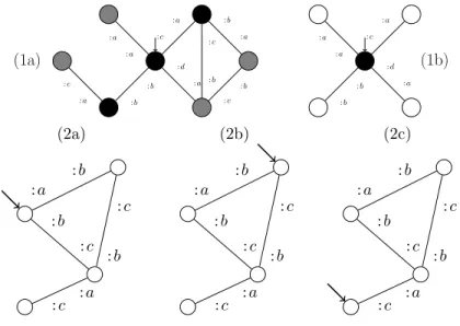
2.2. GENERALIZED CAYLEY GRAPHS 19 (1a) : a : a : c : a : b : b : d : a : b : a : b : c : c : b : a : c (1b) : a : a : c : a : b : b : d : a (2a) : a : b : c : b : b : c : a : c (2b) : a : b : c : b : b : c : a : c (2c) : a : b : c : b : b : c : a : c

Figure 2.2: Operations over pointed graphs modulo. (1) From X to X0_:

taking the subdisk of radius 0. In general the neighbours of radius r are just those vertices which can be reached in r steps starting from the origin, whereas the disk of radius r, written Xr_{, is the subgraph induced by the}

neighbours of radius r + 1, with labellings restricted to the neighbours of radius r and the edges between them. (2a) A pointed graph modulo X. (2b) Xab the pointed graph modulo X shifted by ab. (2c) Xbc.ac the pointed graph

modulo X shifted by bc.ac, which also corresponds to the graph Xab shifted

by cb.ac. Shifting this last graph by cb.ac = ca.bc produces the graph (2b) again.

TMKK05, BFH87, L¨ow93, EL93, Tae96, Tae97]. They are illustrated by Figure 2.1(a).

Definition 1 (Graph). A graph G is given by

• An at most countable subset V (G) of V , whose elements are called vertices.

• A finite set π, whose elements are called ports.

• A set E(G) of non-intersecting two element subsets of V (G) : π, whose elements are called edges. In other words an edge e is of the form

(22)

{u : a, v : b}, and ∀e, e′ _{∈ E(G), e ∩ e}′ _{6= ∅ ⇒ e = e}′_.

The graph is assumed to be connected: for any two u, v ∈ V (G), there exists v0, . . . , vn∈ V (G), a0, b0. . . , an−1, bn−1 ∈ π such that for all i ∈ {0 . . . n − 1},

one has {vi: ai, vi+1: bi} ∈ E(G) with v0 = u and vn= v.

Definition 2 (Labelled graph). A labelled graph is a triple (G, σ, δ), also denoted simply G when it is unambiguous, where G is a graph, and σ and δ respectively label the vertices and the edges of G:

• σ is a partial function from V (G) to a finite set Σ; • δ is a partial function from E(G) to a finite set ∆.

The set of all graphs with ports π is written Gπ. The set of labelled graphs

with states Σ, ∆ and ports π is written GΣ,∆,π. To ease notations, we

some-times write v ∈ G for v ∈ V (G).

In definition 2 the labelling functions are possibly partial, e.g. a vertex may be potentially stateless. Allowing for this possibility is convenient to describe local rules, which produce vertices and their relations to neighbour vertices, without necessarily having an opinion on the states of the neighbour vertices. A concrete example of this is given in Section 3.2 and Figure 3.4.

We now want to single out a vertex. Definition 3 is illustrated by Figure 2.1(b).

Definition 3 (Pointed graph). A pointed (labelled) graph is a pair (G, p) with p ∈ G. The set of pointed graphs with ports π is written Pπ. The set of

pointed labelled graphs with states Σ, ∆ and ports π is written PΣ,∆,π.

The idea is now to get rid of all the unnecessary information in these graphs. Definition 4 of isomorphism formalizes the notion of vertex renaming in a graph.

Definition 4 (Isomorphism). An isomorphism R is a function from Gπ to

G_π which is specified by a bijection R(.) from V to V . The image of a graph G under the isomorphism R is a graph RG whose set of vertices is R(V (G)), and whose set of edges is {{R(u) : a, R(v) : b} | {u : a, v : b} ∈ E(G)}. Similarly, the image of a pointed graph P = (G, p) is the pointed graph RP = (RG, R(p)). When P and Q are isomorphic we write P ≈ Q, defining

(23)

2.2. GENERALIZED CAYLEY GRAPHS 21 an equivalence relation on the set of pointed graphs. The definition extends to pointed labelled graphs.

Notice that pointed graph isomorphism renames the pointer in the same way as it renames the vertex upon which it points; which effectively means that the pointer does not move. Later we shall introduce a distinct kind of oper-ation, which moves the pointer, not to be confused with this isomorphism. When describing a graph, we do not need to specify the name or the identity of the vertices in order to uniquely describe this graph. In definition 5, we use the notion of isomorphism to get rid of all names in the graph.

Definition 5 (Generalized Cayley graphs). Let P be a pointed (labelled) graph (G, p). The generalized Cayley graph X is eP the equivalence class of P with respect to the equivalence relation ≈. The set of generalized Cayley graphs with ports π is written Xπ. The set of labelled generalized Cayley

graphs with states Σ, ∆ and ports π is written XΣ,∆,π.

These pointed graphs modulo will constitute the set of configurations of the generalized cellular automata that we will consider in this work.

We will need a notion of path in a generalized Cayley graph:

Definition 6 (Path). Given a generalized Cayley graph X, we say that α ∈ Π∗ _{is a path of X if and only if there is a finite sequence α = (a}

ibi)i∈{0,...,n−1}

of ports such that, starting from the pointer, it is possible to traverse the graph according to this sequence. More formally, α is a path if and only if there exists (G, p) ∈ X and there also exists v0, . . . , vn∈ V (G) such that for

all i ∈ {0, . . . , n − 1}, one has {vi : ai, vi+1 : bi} ∈ E(G), with v0 = p and

αi = aibi. Notice that the existence of a path does not depend on the choice

of (G, p) ∈ X. The set of paths of X is denoted by L(X).

Notice that paths can be seen as words on the alphabet Π and thus come with a natural operation ‘.’ of concatenation, a unit ε denoting the empty path, and a notion of inverse path α which stands for mirror of path α. The detailed algebraic structure of the set of paths L(X) of a generalized Cayley graph X is described in Appendix A.

Two paths are equivalent if they lead to same vertex:

(24)

X, we define the equivalence of paths relation, denoted ≡X, on L(X) such

that for all paths α, α′ _{∈ L(X), α ≡}

X α′ if and only if, starting from the

pointer, α and α′ _{lead to the same vertex of X. More formally, α ≡}

X α′ if

and only if there exists (G, p) ∈ X and v1, . . . , vn, v1′, . . . , vn′′ ∈ V (G) such that

for all i ∈ {0 . . . n − 1}, i′ _{∈ {0 . . . n}′ _{− 1}, one has {v}

i: ai, vi+1: bi} ∈ E(G),

{v′

i′ : a′_i′, v′_i′₊₁ : b_i′′} ∈ E(G), with v₀ = p, v₀′ = p, α = (aibi)i∈{0,...,n−1},

α′ _{= (a}′

i′b′_i′)i∈{0,...,n′_−1} and v_n = v_n′. We write ˜α for the equivalence class of

α with respect to ≡X.

For mainly technical reasons, it will often be useful to undo the modulo, i.e. to obtain a canonical instance of a pointed graph modulo.

Definition 8 (Associated graph). Let X be a generalized Cayley graph. Let G(X) be the graph such that:

• The set of vertices V (G(X)) is the set of equivalence classes of L(X); • The edge {˜α : a, ˜β : b} is in E(G(X)) if and only if α.ab ∈ L(X) and

α.ab ≡X β, for all α ∈ ˜α and β ∈ ˜β.

We define the associated graph to be G(X). Conventions. Appendix A proves that:

• a generalized Cayley graph X, • its associated graph G(X)

• the algebraic structure hL(X), ≡Xi

can be viewed as three presentations of the same mathematical object. It further provides an axiomatization of these algebraic structures. Altogether, this justifies the fact that each vertex of this mathematical object can be designated by

• ˜α an equivalence class of L(X), i.e. the set of all paths leading to this vertex starting from ˜ε,

• or more directly by α an element of an equivalence class ˜α of X, i.e. a particular path leading to this vertex starting from ε.

These two remarks lead to the following mathematical conventions, which we adopt for convenience. From now on:

(25)

2.3. BASIC OPERATIONS 23 • ˜α, α will no longer be distinguished. The latter notation will be given the meaning of the former. We shall speak of a “vertex” α in V (X) (or simply α ∈ X).

• It follows that ‘≡X’ and ‘=’ will no longer be distinguished. The latter

notation will be given the meaning of the former. I.e. we shall speak of “equality of vertices” α = β (when strictly speaking we just have

˜ α = ˜β).

In any case, we will make sure that a rigorous meaning can always be recov-ered by placing tildes back.

2.3 Basic operations

2.3.1 Operations on generalized Cayley graphs

For a pointed graph (G, p) non-modulo (see [AD12] for details):

• the neighbours of radius r are just those vertices which can be reached in r steps starting from the pointer p;

• the disk of radius r, written Gr

p, is the subgraph induced by the

neigh-bours of radius r + 1, with labellings restricted to the neighneigh-bours of radius r and the edges between them, and pointed at p.

Notice that the vertices of Gr

p continue to have the same names as they

used to have in G. For generalized Cayley graphs, on the other hand, the analogous operation is:

Definition 9 (Disk). Let X ∈ XΣ,∆,π be a generalized Cayley graph and G

its associated graph. Let Xr_{be f}_Gr

ε. The generalized Cayley graph Xr ∈ XΣ,∆,π

is referred to as the disk of radius r of X. The set of disks of radius r with states Σ, ∆ and ports π is written Xr

Σ,∆,π.

A technical remark is that the vertices of Xr_{no longer have quite the same}

names as they used to have in X. This is because, in a generalized Cayley graph, vertices are designated by those paths that lead to them, starting from the vertex ε, and there were many more such paths in X than there are in its subgraph Xr_{. Still, it is clear that there is a natural inclusion V (X}r_{) ⊆ V (X),}

(26)

e

ε

e

aa

e

bb

g

bb.ac

e

ca

e

da

g

da.cb :a :a :b :b :a :c :c :a :d :a :b :a :c :b :c :b

e

ε

e

aa

e

bb

e

ca

e

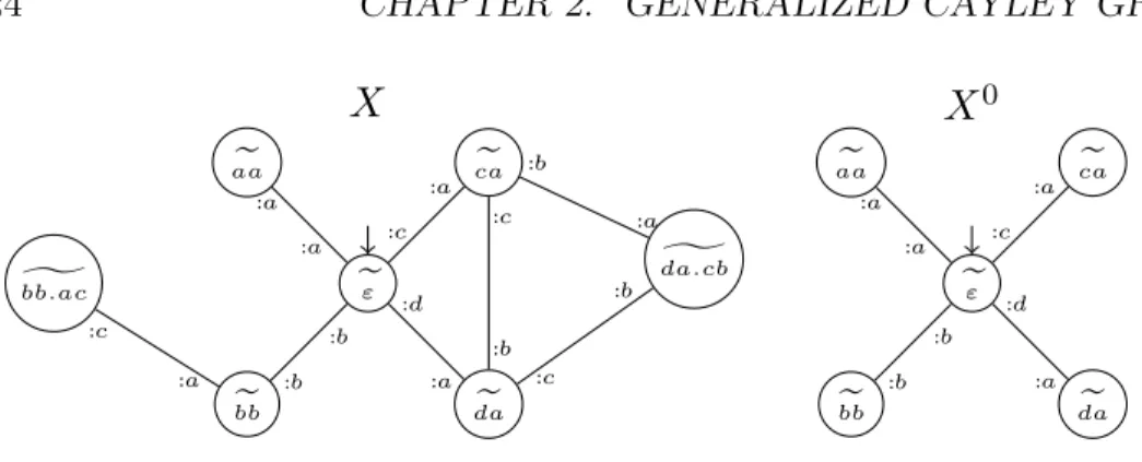
da :a :a :b :b :c :a :d :a

X

0

Figure 2.3: A generalized Cayley graph and its disk of radius 0. Notice that the equivalence classes describing vertices in X0 _{are strict subsets of those in}

X, even though their shortest representative is the same. For instance the path ca.cb is in ˜da in X but is not a path in X0_{, and thus does not belong}

to ˜da in X0_.

u ⊆ u′_{. Thus, we will commonly say that a vertex of u ∈ X}r _{belongs to X,}

even though technically we are referring to the corresponding vertex u′ _{of X.}

Similarly, we will commonly say that a vertex of u′ _{∈ X belongs to X}r _when

we actually mean that there is a unique vertex u of Xr _{such that u ⊆ u}′_.

Definition 10 (Size). Let X ∈ XΣ,∆,π be a generalized Cayley graph. We

say that a vertex u ∈ X has size less or equal to r + 1, and write |u| ≤ r + 1, if and only if u ∈ Xr_{. We denote V (X}r

π) =

S

X∈Xr

πV (X).

It will help to have a notation for the graph where vertices are named rela-tively to some other pointer vertex u.

Definition 11 (Shift). Let X ∈ XΣ,∆,π be a generalized Cayley graph and

G its associated graph. Consider u ∈ X or Xr _{for some r, and consider the}

pointed graph (G, u), which is the same as (G, ε) but with a different pointer. Let Xu be(G, u). The generalized Cayley graph X^ u is referred to as X shifted

by u.

The composition of a shift, and then a restriction, applied on X, will simply be written Xr

u. Whilst this is the analogous operation to Gru over pointed

graphs non-modulo, notice that the shift-by-u completely changes the names of the vertices of Xr

(27)

2.3. BASIC OPERATIONS 25 holds no information about its prior location, u.

We may also want to designate a vertex v by those paths that lead to the vertex u relative to ε, followed by those paths that lead to v relative to u. The following definition of concatenation coincides with the one that is induced by the concatenation of words belonging to the classes u and v:

Definition 12 (Concatenation). Let X ∈ Xπ be a generalized Cayley

graph and G its associated graph. Consider u ∈ X and v ∈ Xu or Xur

for some r. Let G′ _{be the associated graph of (X}

u)v, R be an isomorphism

such that G′ _{= RG, and u.v be R}−1_{(ε). The vertex u.v ∈ X is referred to as}

u concatenated with v.

According to Definition 11, G′ _{and G are isomorphic. Moreover, the}

restric-tion of R−1 _{to V (G}′_{) is uniquely determined; hence definition 12 is sound.}

It also helps to have a notation for the paths to ε relative to u.

Definition 13 (Inverse). Let X ∈ Xπ be a generalized Cayley graph and G

its associated graph. Consider u ∈ X. Let G′ _{be the associated graph of X} u

and R be an isomorphism such that G′ _{= RG, and u be R(ε). The vertex}

u ∈ Xu is referred to as the inverse of u.

Notice the following easy facts: (Xu)v = Xu.v, u.u = ε. Notice also that the

isomorphism R such that G(Xu) = RG(X) maps v to u.v. This last property

suggests that we may define shifts upon graphs (non-modulo) as a certain class of isomorphisms. In order to formalize this notion within the set of graphs without appealing to graphs modulo, we will need that the vertices of our graphs non-modulo be of a particular form.

2.3.2 Operations on graphs

In Section 2.2 we said that a graph G ∈ Gπ would have vertex names in

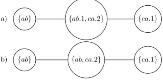
V . But now we shall allow vertices to have names in disjoint subsets of V.S, with S = {ε, 1, 2, . . . , b} a finite set of suffixes. For instance, given some generalized Cayley graph X, having vertices u, v in V (X), we may build some graph G having vertices {v}, {u.1}, {u.3, v.1} . . . i.e. subsets of V (X).S. Later, {u.1} will be interpreted as the vertex which is ‘the first successor of u’, {u.3, v.1} as the vertex which is ‘the first successor of v and the third successor of u’, {v} as the vertex which is ‘the continuation of v’. Disjointness is just to keep things tidy: one cannot have a vertex which is the

(28)

first successor of u ({u.1}, say) coexisting with another which is the ‘the first successor of u and the second successor of v’ ({u.1, v.2}, say) — although some other convention could have been used. Still, some form of suffixes is necessary in order to provide just the little, extra naming space that is needed in order to create new vertices. Figure 2.4 illustrates this restriction over the vertices names.

{ab} {ab.1, ca.2} {ca.1}

{ab} {ab, ca.2} {ca.1}

a)

b)

Figure 2.4: a) Is a valid graph as all its vertices names are disjoint subsets. However, b) is not valid as vertices names {ab} and {ab, ca.2} intersect.

Definition 14 (Shift isomorphism). Let X ∈ Xπ be a generalized Cayley

graph. Let G ∈ Gπ be a graph that has vertices that are disjoint subsets of

V (X).S or V (Xr_{).S for some r. Consider u ∈ X. Let R be the isomorphism}

from V (X).S to V (Xu).S mapping v.z 7→ u.v.z, for any v ∈ V (X) or V (Xr),

z ∈ S. Extend this bijection pointwise to act over subsets of V (X).S, and let u.G to be RG. The graph u.G has vertices that are disjoint subsets of V (Xu).S, it is referred to as G shifted by u. The definition extends to labelled

graphs.

Definitions 15 and 16 are standard, see [BFH87, L¨ow93] and [AD12], although here again the vertices of G are given names in disjoint subsets of V (X).S for some X. Basically, we need a notion of union of graphs, and for this purpose we need a notion of consistency between the operands of the union:

Definition 15 (Consistency). Let X ∈ Xπ be a generalized Cayley graph.

Let G be a labelled graph (G, σ, δ), and G′ _{be a labelled graph (G}′_{, σ}′_{, δ}′_{), each}

one having vertices that are pairwise disjoint subsets of V (X).S. The graphs are said to be consistent if and only if:

(29)

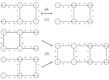
2.3. BASIC OPERATIONS 27 2 3 ε 1 ba.ε ba.1 :d :b :a :c :b :d :c :a :b :a :b :a ab.2 ab.3 ab.ε ab.1 ε 1 :d :b :a :c :b :d :c :a :b :a :b :a (1) ab. 3 ε 1 2 ab.2 ab.1 :a :c :b :d :c :a :d :b :a :b :a :b ab.2 ab.3 ab.ε ab.1 ε 1 :d :b :a :c :b :d :c :a :b :a :b :a 3 ε 1 2 ab.2 ab.3 ab.ε ab.1 :a :c :b :d :c :a :d :b :d :b :a :c :b :d :c :a :a :b :a :b (2)

Figure 2.5: Operations over graphs. (1) A shift of a graph on the vertex ba. The structure of the graph is preserved, only the names of the vertices are changed. The new vertex ε is the former vertex ba. (2) A graph union. Here the two graphs on the left hand side intersect on vertices ε, 1, ab.1 and ab.2. As the two are consistent (e.g. in both graph, vertices ε and ab.2 are connected along an ab edge) their union can be computed, resulting in the right hand side graph.

(ii) ∀x, y ∈ G ∀x′_{, y}′ _{∈ G}′_{∀a, a}′_{, b, b}′ _{∈ π}

({x : a, y : b} ∈ E(G) ∧ {x′: a′, y′: b′} ∈ E(G′_{) ∧ x = x}′_{∧ a = a}′_{) ⇒ (b = b}′_{∧ y = y}′_),

(iii) ∀x, y ∈ G ∀x′_{, y}′ _{∈ G}′_{∀a, b ∈ π} _{x = x}′ _{⇒ δ({x : a, y : b}) = δ}′_({x′_{: a, y}′_:

b}) when both are defined,

(iv) ∀x ∈ G ∀x′ _{∈ G}′ _{x = x}′ _{⇒ σ(x) = σ}′_(x′_{) when both are defined.}

They are said to be trivially consistent if and only if for all x ∈ G, x′ _{∈ G}′

we have x ∩ x′ _{= ∅.}

The consistency conditions aim at making sure that both graphs “do not disagree”. Indeed: (iv) means that “if G says that vertex x has label σ(x), G′ _{should either agree or have no label for x”; (iii) means that “if G says}

(30)

that edge e has label δ(e), G′ _{should either agree or have no label for e”; (ii)}

means that “if G says that starting from vertex x and following port a leads to y via port b, G′ _{should either agree or have no edge on port x : a”.}

Condition (i) is in the same spirit: it requires that G and G′_{, if they have a}

vertex in common, then they must fully agree on its name. Remember that vertices of G and G′ _{are disjoint subsets of V (X).S. If one wishes to take}

the union of G and G′_{, one has to enforce that the vertex names will still be}

disjoint subsets of V (X).S.

Trivial consistency arises when G and G′ _{have no vertex in common: thus,}

they cannot disagree on any of the above.

Definition 16 (Union). Let X ∈ Xπ be a generalized Cayley graph. Let

G be a labelled graph (G, σ, δ), and G′ _{be a labelled graph (G}′_{, σ}′_{, δ}′_{), each}

one having vertices that are pairwise disjoint subsets of V (X).S. Whenever they are consistent, their union is defined. The resulting graph G ∪ G′ _{is the}

labelled graph with vertices V (G) ∪ V (G′_{), edges E(G) ∪ E(G}′_{), labels that}

are the union of the labels of G and G′_.

Finally, recall that for a pointed graph (G, p) non-modulo Gr

p, is the

subgraph induced by the neighbours of radius r + 1, with labellings restricted to the neighbours of radius r and the edges between them, and pointed at p [AD12].

2.4 Topological properties

Having a well-defined notion of disks allows us to define a topology upon X_Σ,∆,π, which is the natural generalization of the well-studied Cantor metric upon cellular automata configurations [Hed69].

Definition 17 (Gromov-Hausdorff-Cantor metrics). Consider the func-tion

d : XΣ,∆,π× XΣ,∆,π −→ R+

(X, Y ) 7→ d(X, Y ) = 0 if X = Y (X, Y ) 7→ d(X, Y ) = 1/2r _otherwise

(31)

2.4. TOPOLOGICAL PROPERTIES 29 The function d(., .) is such that for ǫ > 0 we have (with r = ⌊− log₂(ǫ)⌋):

d(X, Y ) < ǫ ⇔ Xr _{= Y}r_.

It defines an ultrametric distance. Soundness:

[Nonnegativity, symmetry, identity of indiscernibles] are obvious. [Equivalence] d(X, Y ) < ǫ ⇔ d(X, Y ) = 1/2k with k ∈ N ∧ 1/2k < ǫ ⇔ k = min{r ∈ N | Xr _{6= Y}r_{} ∧ 1/2}k < ǫ ⇔r=k−1 Xr = Yr with r ∈ N ∧ 1/2r+1 < ǫ ⇔ Xr _{= Y}r _{with r = ⌊− log} 2(ǫ)⌋.

[Ultrametricity] Consider k such that 1/2k _{= d(X, Z) and l such that}

1/2l _{= d(X, Y ). By definition of the metric X, Z differ only after index k}

and X, Y differ only after index l. Suppose k ≤ l so that Y, Z differ only after index k. But then d(Y, Z) = 1/2k _{which is d(X, Z).}

[Triangle inequality] is obvious from the ultrametricity.

The fact that generalized Cayley graphs are pointed graphs modulo, i.e. the fact that they have no “vertex name degree of freedom” is key to proving the following property. Indeed, compactness crucially relies on the set be-ing “finite-branchbe-ing”, meanbe-ing that the set of possible generalized Cayley graphs, as one progressively enlarges the radius of a disk, remains finite. This does not hold for usual graphs.

Lemma 1 (Compactness). (XΣ,∆,π, d) is a compact metric space, i.e.

ev-ery sequence admits a converging subsequence.

Proof. This is essentially K¨onig’s Lemma. Let us consider an infinite se-quence of graphs (X(n))n∈N. Because Σ and ∆ are finite, and there is an

infinity of elements of (X(n)), there must exist a graph of radius zero X0

such that there is an infinity of elements of (X(n)) fulfilling X(n)0 _{= X}0_.

Choose one of them to be X(n0), i.e. X(n0)0 = X0. Now iterate: because

the degree of the graph is bounded by |π|, and because Σ and ∆ are finite but there is an infinity of elements of (X(n)) having the above property, there must exist a pointed graph of radius one X1 _{such that (X}1₎0 _{= X}0 _{and such}

(32)

that there is an infinity of elements of (X(n)) having X(n)1 _{= X}1_{. Choose}

one of them as X(n1), i.e. X(n1)1 = X1. Etc. The limit is the unique graph

X′ _{having disks X}′k _{= X}k _{for all k.}

Recall the difference in quantifiers between the continuity of a function F over a metric space (X, d):

∀X ∈ X ∀ǫ > 0 ∃η > 0 ∀Y ∈ X, d(X, Y ) < η ⇒ d(F (X), F (Y )) < ǫ, and its uniform continuity:

∀ǫ > 0 ∃η > 0 ∀X, Y ∈ X, d(X, Y ) < η ⇒ d(F (X), F (Y )) < ǫ. Uniform continuity is the physically relevant notion, as it captures the fact that F does not propagate information too fast. In a compact setting, it is equivalent to simple continuity, which is easier to check and is the mathemat-ically standard notion. This is the content of Heine’s Theorem, a well-known result in general topology [FAP90]: given two metric spaces X and Y and F : X −→ Y continuous, if X is compact, then F is uniformly continuous.

The implications of these topological notions for cellular automata were first studied in [Hed69], with self-contained elementary proofs available in [Kar11]. For cellular automata over Cayley graphs a complete reference is [CSC10]. For causal graph dynamics [AD12], these implications had to be reproven by hand, due to the lack of a clear topology in the set of graphs that was considered. Here we are able rely on the topology of generalized Cayley graphs and reuse Heine’s theorem out-of-the-box, which makes the setting of generalized Cayley graphs a very attractive one in order to generalize cellular automata.

2.5 Summary of the results

We constructed a model graph, generalized Cayley graphs, having the fol-lowing properties:

• neighbours of vertices are numbered, with numbering in a finite set π, hence bounding the degree of the graph,

• a particular, pointed, vertex plays the role of origin in the graph, • vertices are named relatively to this origin.

(33)

2.5. SUMMARY OF THE RESULTS 31 We defined several operations over these graphs. In particular, we defined a notion of shift, which consists in moving the origin along a given path in the graph, and a notion of disk. We also endowed the set of generalized Cayley graphs with a compact metric, allowing us to define uniformly continuous transformations over this set.

(34)

(35)

Chapter 3 Causal graph dynamics

Generalizing cellular automata. Now that our configuration space is well defined, we will present our definition of cellular automata over generalized Cayley graphs, namely causal graph dynamics. The main challenge here is to preserve the two definitions of “classical” cellular automata, giving them legitimacy as both physics toy-models and computational models, and to prove their equivalence.

The first two sections of this chapter give two alternative definitions of our model: section 3.1 is based on the notions of causality and homogeneity, while section 3.2 is based on the notion of local rule. Finally, section 3.3 provides a proof of the equivalence between these two definitions.

The content of this chapter is based on [AMN13] and [AM12], co-authored with Pablo Arrighi and Vincent Nesme.

3.1 Causal dynamics

The notion of causality extends the known mathematical definition of cellular automata over grids and Cayley graphs. This extension will have two main features: not only the graphs become arbitrary, but they can also vary in time.

In order to define these causal dynamics, we will need to define three properties over graph transformations. The first two properties, continuity and shift-invariance, are very similar to their equivalent in CA theory, even though their expression is less immediate due to the complexity of the config-uration set. The last property, boundedness, is here to prevent our dynamics

(36)

34 CHAPTER 3. CAUSAL GRAPH DYNAMICS

to locally create an infinite number of new vertices.

The main difficulty we encountered when elaborating an axiomatic def-inition of causality from XΣ,∆,π to XΣ,∆,π (the set of generalized Cayley

graphs), was the need to establish a correspondence between the vertices of X ∈ XΣ,∆,π, and those of its image by a dynamics F , F (X). Indeed,

on the one hand it is important to know that a given u ∈ X has become u′ _{∈ F (X), e.g. in order to express the shift-invariance F (X}

u) = F (X)u′.

But on the other hand since u′ _{is named relative to ε, its determination}

requires a global knowledge of X.

The following analogy provides a useful way of tackling this issue. Say that we were able to place a white stone on the vertex u ∈ X that we wish to follow across the application of the dynamics F . Later, by observing that the white stone is found at u′ _{∈ F (X), we would be able to conclude that u}

has become u′_{. This way of grasping the correspondence between an image}

vertex and its antecedent vertex is a local, operational notion of an observer moving across the dynamics.

Definition 18 (Dynamics). A dynamics (F, R•) is given by

• a function F : XΣ,∆,π → XΣ,∆,π;

• a map R•, with R• : X 7→ RX and RX : V (X) → V (F (X)).

For all X, the function RX can be pointwise extended to sets, i.e. RX :

P_{(V (X)) → P(V (F (X))) maps S to R}_X_{(S) = {R}_X_{(u) | u ∈ S}.}

The intuition is that RX indicates which vertices {u′, v′, · · · } = RX({u, v, · · · }) ⊆

V (F (X)) will end up being marked as a consequence of {u, v, · · · } ⊆ V (X) being marked. Now, clearly, the set {(X, P(V (X))) | X ∈ XΣ,∆,π} is

iso-morphic to XΣ′_,∆,π with Σ′ = Σ × {0, 1}. Hence, we can define the function

F′ _{that maps (X, S) ∼}_{= X}′ _{∈ X}

Σ′_,∆,π to (F (X), R_X(S)) ∼= F′(X′) ∈ X_Σ′_,∆,π,

and think of a dynamics as just this function F′ _{: X}

Σ′_,∆,π → X_Σ′_,∆,π. This

alternative formalism will turn out to be very useful.

Definition 19 (Shift-invariance). A dynamics (F, R•) is said to be

shift-invariant if and only if for every X and u ∈ X, v ∈ Xu,

• F (Xu) = F (X)RX(u)

(37)

3.1. CAUSAL DYNAMICS 35 The second condition expresses the shift-invariance of R•. Notice that

RX(ε) = RX(ε).RX(ε); hence RX(ε) = ε.

In the F′ _{: X}

Σ′_,∆,π → X_Σ′_,∆,π formalism, the two above conditions are

equiv-alent to just one: F′_(X

u) = F′(X)RX(u).

Definition 20 (Continuity). A dynamics (F, R•) is said to be continuous

if and only if:

• F : XΣ,∆,π → XΣ,∆,π is continuous,

• For all X, for all integer m, there exists an integer n such that for all X′_{, X}′n _{= X}n _{implies dom R}m

X′ ⊆ V (X′n), dom R_Xm ⊆ V (Xn) and

Rm

X′ = Rm_X.

where Rm

X denotes the partial map obtained as the restriction of RX to the

codomain F (X)m_{, using the natural inclusion of F (X)}m _{into F (X).}

The second condition expresses the continuity of R•. It can be reinforced

into uniform continuity: for all m, there exists n such that for all X, X′_,

X′n _{= X}n _{implies R}m

X′ = Rm_X.

Indeed, in the F′ _{: X}

Σ′_,∆,π → X_Σ′_,∆,π formalism, the two above conditions are

equivalent to just one: F′ _{continuous. But since continuity implies uniform}

continuity upon the compact space XΣ′_,∆,π, it follows that F′ is uniformly

continuous, and thus the reinforced second condition. We need one third, last condition:

Definition 21 (Boundedness). A dynamics (F, R•) from XΣ,∆,π to XΣ,∆,π

is said to be bounded if and only if there exists a bound b such that for all X, for all w′ _{∈ F (X), there exists u}′ _{∈ im R}

X and v′ ∈ F (X)bu′ such that

w′ _{= u}′_.v′_.

With the help of these three conditions, we can state our main definition: Definition 22 (Causal dynamics). A dynamics is causal if it is shift-invariant, continuous and bounded.

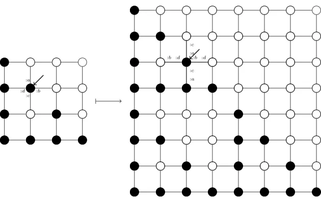
Example: The inflating grid. An example of causal dynamics is the in-flating grid dynamics illustrated in Figure 3.1. In the inin-flating grid dynamics each vertex gives birth to four distinct vertices, such that the structure of the initial graph is preserved, but inflated. The graph has maximal degree

(38)

4, and the set of ports is π = {a, b, c, d}, vertices and edges are unlabelled. For this dynamics, the R• operator is defined as follows:

RX(u0· u1· · · un) = R(u0) · R(u1) · · · R(un)

where R is the function acting on letters in π2 _{described in the following}

table: u ∈ π2 _R(u) aa aa.db ab ab.db.ac ac ac.ac ad ad.bd ba bd.ba.db bb bd.bb.db.ac bc bd.bc.ac bd bd.bd ca ca.ca cb ca.cb.db cc ca.cc.db.ac cd ca.cd.ac da da db db.db dc dc.db.ac dd dd.ac

For instance, if two vertices are sep-arated by a single edge cb in X, then moving the pointer from the first one to the second one will re-sult in moving the pointer along the path R(cb) = ca.cb.db in F (X).

Lemma 2 (Bounded inflation). Consider a causal dynamics F from XΣ,∆,π

to XΣ,∆,π. There exists a bound b such that for all X and u ∈ Xr, we have

|RX(u)| ≤ (r + 1)b.

Proof. Let ac ∈ Π, and let E the subset of XΣ,∆,π of those X such that

ac ∈ X. E is closed — any sequence of elements of E converging in XΣ,∆,π

converges in E — and XΣ,∆,π is compact, therefore E is compact. By

con-tinuity, the function X 7→ |RX(ac)| is continuous from E to N; since E is

compact, it must be bounded. The result then follows from the triangle inequality and shift-invariance.

(39)

3.1. CAUSAL DYNAMICS 37 :a :d :c :b :a :c :c :a :d :b :b :d

Figure 3.1: The inflating grid dynamics. Each vertex splits into 4 vertices. The structure of the grid is preserved. For this precise graph, all edges are connected to ports as stipulated on the pointed vertex (port : a on top, : b on the right, : c on the bottom and : d on the left).

(40)

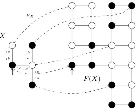
38 CHAPTER 3. CAUSAL GRAPH DYNAMICS : c : d : b : c : a : b : c : a

X

F

(X)

RX

Figure 3.2: To each original vertex of X, RX associates a vertex of F (X)

within the square of four it creates. More precisely, it is mapped to that of the four vertices whose ports a and d get out of the square.

(41)

3.2. LOCALIZABLE DYNAMICS 39

3.2 Localizable dynamics

The notion of localizability of a dynamics F captures exactly the same idea as the constructive definition of a cellular automata, namely that F arises as a single local rule f applied synchronously and homogeneously across the input graph.

The general idea is that the local rule f looks at a portion of the generalized Cayley graph X (a disk Xr_{) and produces a piece of graph G = f (X}r_).

The same is done synchronously at every location u ∈ X producing pieces of graph G′ _{= f (X}r

u). The produced pieces must be consistent (see Subsection

2.3.2) so that we take their union. Their union is a graph, but taking its modulo leads to a generalized Cayley graph F (X).

We now formalize this idea.

First, we must make sure that a local rule is an object that adopts the same naming conventions for vertices as those of the basic graph operations of Subsection 2.3.2.

Definition 23 (Dynamics non-modulo). A function f from XΣ,∆,π to

G_Σ,∆,π is said to be a dynamics if and only if for all X the vertices of f (X) are disjoint subsets of V (X).S, and ε ∈ f (X).

Intuitively, the integer z ∈ S stands for the ‘successor number z’. Hence the vertices designated by {1}, {2} · · · are successors of the vertex ε, whereas {ε} is its ‘continuation’, i.e. its direct descendant. The vertices designated by {ab.1}, {ab.2} · · · are successors of its neighbour ab ∈ Xr_{. A vertex named}

{1, ab.3} is understood to be both the first successor of vertex ε and the third successor of vertex ab. Recall also that ε, just like ab, are not just words but entire equivalence classes of these words, i.e. elements of V (X).

Next, we disallow local rules that would suddenly produce an infinite graph. Definition 24 (Boundedness non-modulo). A function f from Xr

Σ,∆,π

to GΣ,∆,π is said to be bounded if and only if for all X, the graph f (X) is

finite.

Finally, we make sure that the different pieces of graphs that are produced by the local rule are consistent with one another.

Definition 25 (Local rule). A function f from XΣ,∆,π to GΣ,∆,π is a local

(42)

• For any disk Xr+1 _{and any u ∈ X}0 _{we have that f (X}r_{) and u.f (X}r u)

are non-trivially consistent.

• For any disk X3r+2 _{and any u ∈ X}2r+1_{we have that f (X}r_{) and u.f (X}r u)

are consistent.

It is clear that we do not need to formulate any consistency condition beyond u ∈ X2r+1_{, because f (X}r_{) and u.f (X}r

u) then become trivially

con-sistent, as they share nothing in common, see Figure 3.3. The only subtlety in Definition 25 is to impose that within u ∈ X0_{, the produced pieces of}

graphs f (Xr_{) and u.f (X}r

u) be non-trivially consistent, i.e. consistent and

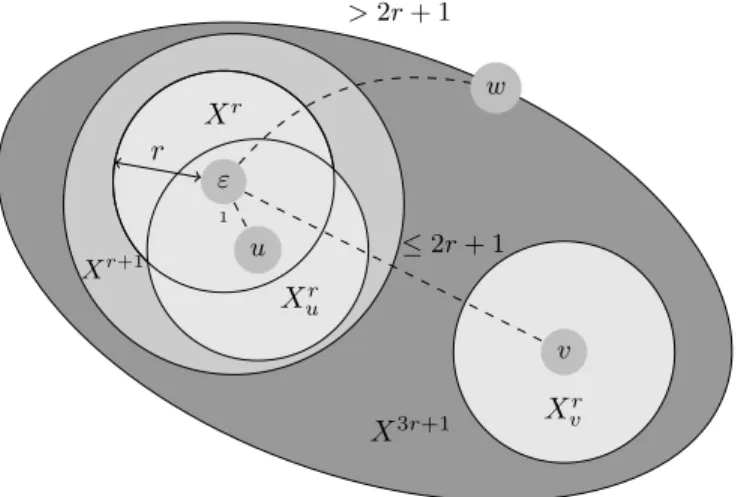
overlapping (see Figure 3.3). The point here is to enforce the connectedness of the union of the pieces of graphs via a local, syntactic restriction. To

illus-ε w Xr > 2r + 1 r u 1 Xr u Xr+1 v Xr v ≤ 2r + 1 X3r+1

Figure 3.3: The consistency conditions for a local rule. The drawing rep-resents disks of a generalized Cayley graph X upon which a local rule f of radius r will be applied. f (Xr_{) and u.f (X}r

u) have to be non-trivially

consis-tent since ε and u are at distance 1. f (Xr_{) and v.f (X}r

v) have to be consistent

but their intersection is allowed to be empty. f (Xr_{) and w.f (X}r

w) will be

trivially consistent as they are to far to interact in one time step. The disk Xr+1 _{is large enough to check all the non-trivial consistency conditions, as}

it contains first neighbours and their r-disks. The disk X3r+1 _{is enough to}

check all the consistency conditions, as it contains all the 2r + 1 neighbours and their r-disks.

(43)

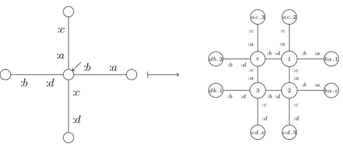
3.2. LOCALIZABLE DYNAMICS 41 trate the concept of local rule, we will now describe a local rule implementing the inflating grid dynamics. The local rule is of radius zero: it “sees” the neighbour vertices and nothing more. In the standard case the local rule is applied on a vertex surrounded by four neighbours. It then generates a graph of twelve vertices, each with particular names (see Figure 3.4). In particular cases, when less than four neighbours are present, the rule generates a graph of 10, 8, 6 or 4 vertices, each with particular names (see Figure 3.5). The local rule is not exhaustively described here, since there exists 625 different neighbourhoods of radius 0. In any case, all generated vertex names are care-fully chosen, so that when taking the union of all the generated subgraphs, the name collisions lead to the desired identification of vertices (see Figure 3.6). :b :a :d :b :a :c :c :d ε 1 2 3 ac.3 ac.2 ba.1 ba.ε cd.ε cd.3 db.2 db.1 :a :c :b :d :a :c :b :a :c :a :b :a :c :d :d :b :a :c :c :d :d :b :d :b

Figure 3.4: Standard case of the inflating grid local rule. The left-hand-side of the rule is a generalized Cayley graph of form X0

u (a disk of radius 0). The

right-hand-side is a graph whose vertex names are subsets of V (X0

u).S. Here

they are just singletons, curly brackets are dropped: e.g. we wrote ac.3 for {ac.3}, which should be understood as “the third successor of my neighbour on edge ac”.

Definition 26 (Localizable function). A function F from XΣ,∆,π to XΣ,∆,π

is said to be localizable if and only if there exists a radius r and a local rule f from Xr

(44)

42 CHAPTER 3. CAUSAL GRAPH DYNAMICS :d :b :a :c ε 1 2 3 ac.3 ac.2 db.2 db.1 :a :c :b :d :a :c :c :a :d :b :a :c :d :b :d :b

Figure 3.5: A particular case of the inflating grid local rule. class modulo isomorphism, of the pointed graph

[

u∈X

u.f (Xr u)

with ε taken as the pointer.

3.3 Equivalence theorem

The following theorem shows that the constructive definition (localizable functions) is in fact equivalent to the mathematical, axiomatic definition (causal dynamics).

Theorem 1 (Causal is equivalent to localizable). Let F be a function from XΣ,∆,π to XΣ,∆,π. The function F is localizable if and only if there exists

R• such that (F, R•) is a causal dynamics.

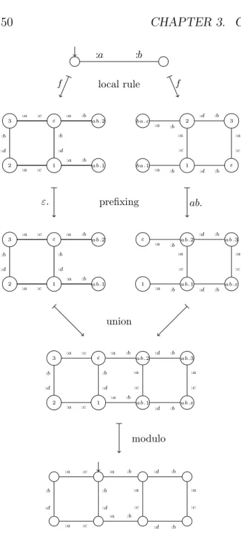
Proof. [Loc.⇒Caus.] Let F : XΣ,∆,π → XΣ,∆,π be a localizable dynamics

with local rule f from Xr

Σ,∆,π to GΣ,∆,π. F (X) is the equivalence class, with

ε taken as the pointer vertex, of the graph H(X) =Su.f (Xr u).

[Dynamics] Using the dynamicity of the local rule f , for all Xr _{we have}

ε ∈ f (Xr_{). Therefore, for all u ∈ X, we have u ∈ u.f (X}r_{) and thus}

Algorithmical and mathematical approaches of causal graph dynamics

HAL Id: tel-01188690

https://tel.archives-ouvertes.fr/tel-01188690

Algorithmical and mathematical approaches of causal

graph dynamics

Simon Martiel

To cite this version:

UNIVERSIT´

E NICE SOPHIA ANTIPOLIS

ECOLE DOCTORALE STIC

TH`

ESE

Simon MARTIEL

Approches informatique et math´

ematique

des dynamiques causales de graphes

Abstract

English

Fran¸cais

Remerciements

Contents

Chapter 1

Introduction

How to read this thesis?

Chapter 2

Generalized cayley graphs

2.1

Brief overview.

2.2

Generalized Cayley Graphs

2.3

Basic operations

2.3.1

Operations on generalized Cayley graphs

e

e

e

g

e

e

g

e

e

e

e

e

X

X

2.3.2

Operations on graphs

2.4

Topological properties

2.5

Summary of the results

Chapter 3

Causal graph dynamics

3.1

Causal dynamics

X

F

(X)

3.2

Localizable dynamics

3.3

Equivalence theorem